Speed-dating and simulation data explain the discrepancy between stated and revealed mate preferences

Abstract

There is little evidence in speed-dating studies that stated preferences – what people say they prefer in a partner – are associated with revealed preferences – what people actually find attractive in a partner. In Study 1, a high-powered speed-dating study (n = 1145) revealed that four out of nine traits provided evidence of a correspondence between stated and revealed preferences. In Study 2, simulations based on the constraints of Study 1’s speed-dating design showed that when attractiveness depends on multiple independent traits, the stated preference for an individual trait can only be, on average, minimally related to the revealed preference for that trait. In Study 3, we investigated methods that simultaneously combine multiple traits when testing the association between stated and revealed preferences (e.g. Euclidean distance, pattern metric). All four omnibus methods indicated an apparent association between stated and revealed preferences in our speed-dating data. However, additional analyses and permutation tests suggest that these significant associations reflect statistical artefacts rather than true correspondences. We conclude that detecting any association between stated and revealed preferences will be difficult under realistic assumptions about the number of traits involved in partner evaluation. In this light, we discuss previous findings and provide suggestions for future studies in this vein.

Plain Language Summary

There is little evidence in speed-dating studies that stated preferences – what people say they prefer in a partner – are associated with revealed preferences – what people actually find attractive in a partner. In three studies, we show that when people evaluate partners on multiple traits, any correspondence between stated and revealed preferences will statistically be very difficult to detect, even when overall attractiveness judgements are driven by stated preferences. In this light, we discuss previous findings and provide suggestions for future studies in this vein.

General Introduction

We have preferences for almost everything in life, and there is the implicit assumption that we act according to these preferences. From an evolutionary perspective, the choice of a romantic partner is one of the most important decisions an individual can make: it determines the genetic makeup of one’s offspring and can affect the resources and protection they receive. Mate preferences are thought to be an adaptation that guides individuals to choose high-fitness mates (e.g. Darwin, 1859). Assuming that fitness is heritable, an individual who chooses a high-fitness mate will tend to have fitter offspring than if they had chosen randomly, thereby increasing the likelihood of the individual’s genes being passed on to subsequent generations.

Much of human mate attraction research relies on stated preferences (e.g. Buss, 1989; Fletcher et al., 1999) – the traits and attributes that an individual states they desire in an ideal partner (although we later discuss that these preferences are not well defined). This body of research assumes that preferences have evolved to guide mate selection, and we would expect that stated preferences should correspond with revealed preferences – which we broadly define as preferences that are revealed by mate choice or attraction.

A focus of mate attraction research is whether stated preferences correspond with revealed preferences (often referred to as predictive validity (Eastwick et al., 2019)). This question is not well-defined in the literature and broadly refers to whether the match, similarity, fit, or congruence between single (or multiple) stated preferences and a partner’s trait rating (or ratings) is associated with positive romantic outcomes (e.g. attraction, romantic partner selection) (Conroy-Beam et al., 2022; Eastwick et al., 2019). From this point onwards, we will refer to this estimand as the correspondence between stated and revealed preferences.

While there is an expectation that stated preferences correspond with revealed preferences, there has been little evidence for such correspondence in speed-dating studies (e.g. Eastwick, 2009; Eastwick, Eagly, et al., 2011; Eastwick et al., 2013; Eastwick & Finkel, 2008; Li et al., 2013; Sparks et al., 2020; Valentine et al., 2020; Wu et al., 2018). Here, we review the current state of findings in speed-dating research as well as the analysis methods used to achieve such findings.

Trait-by-trait methods

The level metric is a trait-by-trait method commonly used to assess the correspondence between stated and revealed preferences (e.g. Eastwick, Eagly, et al., 2011; Li et al., 2013; Wood & Brumbaugh, 2009). We call this a trait-by-trait method because it only considers the attributes (i.e. stated preference and trait rating) for a single trait within a single analysis. The level metric measures the moderation effect of an individual’s stated preference on the association between the partner’s trait rating and romantic outcomes (e.g. overall attractiveness ratings, or agreement to go on another date (Eastwick et al., 2019; Eastwick & Neff, 2012)). For example, if individuals with a higher stated preference for facial attractiveness also tended to show a stronger association between facial attractiveness ratings and overall attractiveness ratings relative to individuals with a lower stated preference for facial attractiveness, we could conclude that there was a correspondence between stated and revealed preferences for facial attractiveness.

Speed-dating paradigms

Using the level metric, speed-dating studies have found little to no evidence of a correspondence between stated and revealed preferences. For example, Eastwick and Finkel (2008) investigated the traits physical attractiveness, earning prospects, and personability along with the outcomes romantic desire, chemistry, and saying yes to a date. Stated preferences did not moderate the association between participant ratings of a partner’s traits and different romantic outcomes (i.e. there was no correspondence between stated and revealed preferences across any traits). Further, Eastwick, Eagly et al. (2011) found no association between stated and revealed preferences for physical attractiveness in a speed-dating context. Similarly, Wu et al. (2018) found that stated ingroup preferences did not significantly predict revealed ingroup preferences in Asian–Americans participating in a speed-dating study.

Sparks et al. (2020) detected no correspondence between stated and revealed preferences in an unrestricted, one-hour blind-date-style study. Participants were ‘yoked’ with another same-sex participant such that both individuals rated their blind-date partners according to both their own most valued traits, as well as those of the ‘yoked’ participant. There was no difference in the effect size of the revealed preferences in the self-valued traits relative to that of the yoked participant (n = 138). Given the longer interaction time, these results suggest that the duration of the date is unlikely a contributing factor in the lack of correspondence seen in speed-dating studies.

In contrast, Li et al. (2013) found a significant correspondence between stated and revealed preferences for social status (n = 142) and physical attractiveness (n = 93) in a speed-dating context. Their methodology differed from typical speed-dating studies in that the speed-dating partners were chosen by the researchers to ensure that the participants only met with two low-and two medium-trait individuals to increase statistical power. Li et al. (2013)’s study demonstrated that participant traits had to be exaggerated to facilitate the detection of such an effect, while unmanipulated dating pools in past speed-dating studies did not tend to find the same correspondence between stated and revealed preferences (e.g. Eastwick et al., 2013).

More recently, Valentine et al. (2020) found a significant correspondence between stated and revealed preferences for the trait warmth-trustworthiness in a speed-dating paradigm (n = 216). The significant effect obtained in this study may be attributed to a larger sample size (relative to past studies), as well as the larger number of interactions within each speed-dating event yielding a larger number of speed-dating observations.

Overall, the limited positive evidence from Li et al. (2013) and Valentine et al. (2020) suggests that if a correspondence between stated and revealed preferences does exist, high-powered studies are required to detect such effects. However, with few positive findings among a large body of negative speed-dating studies (Eastwick, Eagly, et al., 2011; Eastwick et al., 2013; Eastwick & Finkel, 2008; Sparks et al., 2020; Wu et al., 2018), some researchers have taken these null results to indicate that stated preferences are not informative of revealed preferences (Campbell & Stanton, 2014; Eastwick et al., 2013).

Hypothetical and couple paradigms

Other paradigms yield results more favourable to the possibility of a correspondence between stated and revealed preferences. For instance, we see evidence from the level metric when participants rate portrayals of hypothetical partners (e.g. DeBruine et al., 2006; Wood & Brumbaugh, 2009). However, studies using the hypothetical paradigm are problematic due to the abstract manner in which information regarding a potential partner is presented (e.g. images, profiles, vignettes). These stimuli only vary across a few dimensions of interest and do not capture the mate-attraction complexity involved in evaluating a potential partner.

We also see correspondence in studies that investigate couples in committed relationships (e.g. Campbell et al., 2013; Eastwick, Finkel, & Eagly, 2011; Fletcher et al., 1999). However, several longitudinal studies suggest that individuals in relationships adjust their preferences over time (Driebe et al., 2023). Specifically, there is evidence that individuals lowered their stated preferences when their partner fell short of initial stated preferences (Gerlach et al., 2019). Selection bias may also explain the observed effect; if stated preferences related not to initial choice but to the likelihood of relationship dissolution, then couples consisting of individuals unmatched on stated preferences would be less likely to participate in a relationship study (Gerlach et al., 2019).

Evaluating the speed-dating paradigm

While we acknowledge that speed-dating paradigms do not completely mimic natural courtship behaviour, this approach offers many advantages over the aforementioned research paradigms. This paradigm allows us to efficiently collect data using short dates between many people in a live, controlled environment. A common criticism is that the ‘speed’ in speed-dating prevents the accurate assessment of internal traits that are only likely to be revealed over time (e.g. kindness and understanding (Buss, 1989)). However, there is evidence that initial speed-dating ratings are predictive of longer-term romantic interest and romantic outcomes (Baxter et al., 2022). In-person interactions allow individuals to experience more complex facets of an individual compared to a simplified portrayal (e.g. an image). Participants can also control the level and extent of personal interests shared with their partner which can increase the amount of attraction-relevant information that is communicated over a controlled period of time. Individual self-reports are also less likely to be influenced by cognitive dissonance since there is no existing commitment to each speed-dating partner, and therefore we prevent the possibility that individuals may adjust their preferences to suit the traits of a potential partner that they are with/attracted to (e.g. Gerlach et al., 2019).

Do stated preferences inform revealed preferences?

In all, the inconsistencies in findings across these paradigms call into question whether stated preferences predict romantic behaviour. And if they do, then why are these effects so difficult to detect (e.g. Li et al., 2013; Valentine et al., 2020)? Given that there is a genetic basis for stated preferences (Verweij et al., 2012; Zietsch et al., 2012) and there is a cross-cultural consensus on traits desired in an ideal partner (Buss, 1989; Walter et al., 2020), then we would expect that preferences are an adaptation relevant to mate choice. Therefore, a major unresolved issue in mate preference research is the lack of evidence demonstrating that these preferences translate to actual mate selection. Here, we aim to clarify the situation in several ways.

Ambiguity in stated preference measures

Stated preferences have typically been measured in one of two ways. We call the first type preference importance: this measures the extent to which an individual finds it important that a partner possesses a certain quality or trait, for example, ‘Participants rated the importance of [various] characteristics in an ideal romantic partner on a scale from 1 (not at all) to 9 (extremely)’ (Eastwick, 2009). The second measure we call preference level: this measures the preferred level of a trait that an individual’s ideal partner would possess, for example, ‘Each preference variable was rated on a 7-point bipolar adjective scale with each pole representing extreme levels of the relevant trait, for instance “very unkind” to “very kind”’. (Conroy-Beam & Buss, 2017).

While preference importance and preference level measures for the same trait are correlated (.55 ≤ r ≤ .71, see Supplemental Materials), these two measures are conceptually distinct (Conroy-Beam et al., 2016; Driebe et al., 2023). Preference importance relates to the extent to which a partner’s trait is considered in the evaluation of overall attractiveness, whereas preference levels relate to the level of a trait desired in an ideal partner. Some attraction studies have measured preference importance (e.g. Eastwick, 2009; Eastwick & Neff, 2012; Lam et al., 2016; Li et al., 2013; Valentine et al., 2020), while others have measured preference level (e.g. Botwin et al., 1997; Conroy-Beam, 2021; Conroy-Beam & Buss, 2017; Eastwick, Eagly, et al., 2011; Eastwick, Finkel, & Eagly, 2011; Wu et al., 2018). However, it is possible that these preference types could have implications for how the correspondence between stated and revealed preferences should be assessed (Conroy-Beam et al., 2022).

Stated preferences and analyses

The level metric relies on the implicit assumption that stated preferences are linearly proportional to revealed preferences; that is, if stated preferences correspond to revealed preferences, then a higher stated preference is linearly associated with a higher revealed preference (Conroy-Beam & Buss, 2020). This assumption makes sense for preference importance, but not for preference level. We can imagine that as preference importance increases, the importance should be proportional to the increase in the association between the trait rating and overall attractiveness. But for preference level, no such linear relationship makes sense. A partner can deviate from the desired trait level in either direction (e.g. higher or lower than the desired trait level), so we cannot sensibly use the linear interaction between the stated preference level and trait level to predict overall attractiveness. Inappropriate use of the level metric of the latter kind in past studies may have contributed to null findings in the literature (e.g. Eastwick, Eagly, et al., 2011; Wu et al., 2018).

Since preference levels lend themselves to preference matching (e.g. a partner should be the most attractive when their traits match your preference levels), we suggest that the Euclidean distance between stated preference and trait rating can be used to investigate the correspondence between stated and revealed preferences. The Euclidean distance is a measure of distance between coordinates in multidimensional space. In a mate selection context, the Euclidean distance is a measure of preference fulfilment, where the number of dimensions reflects the number of traits assessed (e.g. Conroy-Beam, 2018; Conroy-Beam & Buss, 2017). Euclidean distance is a non-linear measure suited for preference matching; distance is minimised when the preference level is equal to the rating given, and the distance increases if the trait exceeds or falls below the preference level. (There is no clear way to assess a distance between a trait’s preference importance and its rated level in a partner since the desired level of the trait is not specified.) If stated preferences do in fact correspond to revealed preferences, then we would expect a negative association between the Euclidean distance (between a preference and trait rating) with overall attractiveness scores.

We propose a one-dimensional Euclidean distance measure (i.e. the absolute difference between a preference level and its corresponding trait rating) as a suitable trait-by-trait alternative to the level metric when preference levels are measured. This approach has advantages over a similar method called the direct-estimation method (Campbell et al., 2013) where participants rate the extent to which their partner matches their stated preferences (Fletcher et al., 2020). The direct-estimation method can be subject to biases given that participants are explicitly stating the extent to which their partner matches their preferences, and so the direct-estimate measure may correlate highly with perceptions (or ratings of their partners) (Eastwick et al., 2019; Fletcher et al., 2020).

Trait type

The type of preference measure must also be appropriate for the type of trait that is measured. It only makes sense to measure preference importance for universally desirable traits (see Buss (1989)) as it is assumed that the revealed preferences for these traits are in the positive direction (i.e. higher physical attractiveness in a partner is associated with higher romantic attraction overall). However, for idiosyncratic trait preferences (e.g. extraversion), revealed preferences may be in opposite directions: one individual may find high extraversion attractive, whereas another may find low extraversion (i.e. introversion) attractive. It is not meaningful to measure preference importance in these instances because asking, ‘How important is extraversion in an ideal partner?’ is unanswerable for someone for whom introversion is an important trait in an ideal partner. In contrast, preference level items would capture idiosyncratic preferences well – the preferer of introverts can directly state their desired extraversion level (i.e. low).

Human mate choice is complex

Another potential explanation for the apparent lack of correspondence between stated and revealed preferences is the multivariate nature of mate evaluation (Conroy-Beam & Buss, 2020; Conroy-Beam et al., 2022). Individuals evaluate potential partners across multiple traits (Lee et al., 2014). Assuming humans do indeed use stated preferences to evaluate mates, and mate evaluation involves multiple independent traits, then it is mathematically inevitable that, on average, a single stated preference will explain only a small amount of variance in the overall evaluation of a potential partner. (Note that intercorrelated traits and variation in the importance of different trait preferences could still allow for substantial contributions of some individual trait preferences.). For example, a partner may rate highly in one highly preferred trait but may be lacking in many other traits, and in turn, it can reduce a partner’s overall attractiveness score. The consideration of simultaneous traits limits the apparent effects of individual mate preferences on attraction and mate choice (Conroy-Beam & Buss, 2020). This would explain why the level metric – which assesses the correspondence between stated and revealed preferences on a trait-by-trait basis – could often yield null results, especially in relatively small sample sizes.

Omnibus measures

Some past attraction studies have investigated measures that simultaneously consider multiple preferences and trait ratings; we call these omnibus measures. These measures have included the pattern metric (Eastwick, Finkel, & Eagly, 2011; Fletcher et al., 1999, 2000), multidimensional Euclidean distance (Conroy-Beam, 2018; Conroy-Beam & Buss, 2016, 2017), and trait appeal (or weighted sum) (Brandner et al., 2020; Conroy-Beam et al., 2022).

While it is intuitive to consider omnibus measures as an alternative approach to traditional trait-by-trait approaches, there has been little consideration of the assumptions and biases implicitly associated with their use. When multiple preferences and trait ratings are combined to create an omnibus measure (e.g. the pattern metric, Euclidean distance), the resulting value can drastically oversimplify or fail to fully represent the intended nuanced combination of the input values. Here, we will describe the aforementioned omnibus measures, as well as identify potential limitations.

Raw and corrected pattern metric

The (raw) pattern metric (also known as ‘ideal-perception consistency’, ‘profile correlation’, ‘pattern match’, and ‘Q’) measures the extent to which an individual’s preferences align with the trait ratings of a (potential) partner (Eastwick et al., 2011; Edwards, 1994; Fletcher et al., 1999, 2000). For example, if an individual prefers intelligence over facial attractiveness in a partner, the partner would be a better match if she is more intelligent than she is facially attractive. The raw pattern metric is calculated using the within-person correlations between an individual’s stated preferences and their trait ratings of potential partners across multiple traits (and then typically transformed using a Fisher’s Z transformation).

The intended purpose of the pattern metric is to assess the extent that the pattern of an individual’s preferences matches the pattern of partner ratings. Either preference levels or importances are relevant measures against which rating patterns could be assessed. We note, though, that the original use of the pattern metric in an attraction context involved preference importances (Fletcher et al., 1999, 2000).

To date, few studies have evaluated the pattern metric in a live interaction context (e.g. speed-dating), and such studies have found no association between the pattern metric and romantic evaluation ratings (Eastwick & Finkel,2008 ¹ ; Eastwick, Finkel, & Eagly, 2011). The pattern metric also did not significantly predict romantic interest in contexts where single participants rated opposite-sex individuals from their daily lives (Eastwick, 2009) or individuals they wished to be in a relationship with (Eastwick, Finkel, & Eagly, 2011).

In relationship contexts, the pattern metric has been associated with relationship quality and satisfaction (Eastwick, Finkel, & Eagly, 2011; Fletcher et al., 1999, 2000, 2020 ² ), and the likelihood of reduced breakup (Fletcher et al., 2000). However, as mentioned earlier (see Hypothetical and Couple Paradigms), conclusions from relationship studies may be contaminated by participant self-selection bias as well as individuals in relationships tending to change their preferences over the course of their relationship (Driebe et al., 2023; Gerlach et al., 2019).

A commonly identified limitation of the pattern metric is that the measure can be conflated with the average desirability of the items used in the calculation of the pattern metric, that is, failing to account for the ‘normative desirability’ of these traits (Wood & Furr, 2016). Therefore, any association between the pattern metric and overall attractiveness may be driven by the general desirability of the traits that are being rated. A proposed solution is the corrected pattern metric where each item response is mean-centred to remove the normative desirability of each trait rating or preference (Wood & Furr, 2016).

It is unclear whether the corrected pattern metric is more or less predictive of romantic outcomes than the raw pattern metric. Eastwick et al. (2019) ³ and Eastwick et al. (2022) found that the corrected pattern metric yielded weaker (and non-significant) results relative to the raw pattern metric when predicting romantic outcomes for participants in relationships, while Fletcher et al. (2020) found the opposite pattern of results. There are also inconsistencies across different samples; Lam et al. (2016) found positive and null evidence for the association between the corrected pattern metric and various romantic outcomes in Taiwanese and American couples, respectively. In addition, no such studies have investigated whether the corrected pattern metric holds any predictive validity in face-to-face interactions with non-couples, especially in a speed-dating paradigm.

Euclidean distance

Euclidean distance is used to measure the multidimensional distance between preferences and trait ratings, with the number of dimensions given by the number of traits measured. Euclidean distance has been robustly associated with romantic outcomes in both hypothetical and relationship paradigms. The Euclidean distance measure was the most effective algorithm compared to six other preference fulfilment measures for selecting high-fitness mates over many generations in a simulation (Conroy-Beam, 2018). Euclidean distance was predictive of participant romantic attraction to hypothetical online dating profiles (Conroy-Beam & Buss, 2017). In a relationship paradigm, those in committed long-term relationships had a higher fulfilment of long-term preferences (smaller Euclidean distance) than short-term preferences (Conroy-Beam, 2018). And higher preference fulfilment (via Euclidean distance) was associated with higher relationship quality, commitment, and longer relationship duration (Driebe et al., 2023). However, no studies to date have investigated whether Euclidean distance measures predict ratings of overall attractiveness in a real-life speed-dating context.

Trait appeal

We devised a measure called ‘trait appeal’ which represents the weighted average of partner trait ratings, with each rating weighted according to the individual’s preference importance (we also subtract the midpoint of the rating for reasons explained in the Study 2 methods). An individual’s rating of a highly valued trait should be more influential and weighted more highly compared to other less valued traits, which is then reflected in the resulting trait appeal score for that partner. Given that trait appeal is the multivariate extension of the level metric (see Ambiguity in Stated Preference Measures), we believe that preference importances are the most appropriate preference type for trait appeal calculations.

Trait appeal is a variation of the ‘weighted sum’ measure (also known as ‘importance weighting’). Few studies have evaluated the weighted sum measure in an attraction context, and the findings of these studies have been mixed. Brandner et al. (2020) found that the weighted sum measure outperformed Euclidean distance (and many other measures) in predicting the most attractive hypothetical partner profiles across multiple rounds of decision tasks (each involving two trait profiles). In contrast, Conroy-Beam et al. (2022) found that distance measures (including Euclidean distance) outperformed the weighted sum measure in reproducing pairings of real couples.

The weighted sum method has also received considerable attention in the subjective well-being literature (e.g. Campbell et al., 1976). Rohrer and Schmukle (2018) found that satisfaction scores weighted by an individual’s importance for those domains did not exhibit higher correlation scores with overall life satisfaction measures compared to the unweighted satisfaction scores. Similarly Hsieh and Li (2020), found that satisfaction scores weighted by importance ratings only resulted in significantly higher correlations for one out of three outcome variables compared to unweighted scores. Here, it is clear that there is much confusion regarding the benefit of preference importance weighting across a variety of research areas.

The present study

We aim to clarify the apparent lack of correspondence between stated and revealed preferences in several ways. In Study 1, we investigate whether a correspondence exists using trait-by-trait analyses in a large speed-dating sample (n = 1145). The large sample allows more power to detect and precisely estimate the effect of stated preferences on behaviour. We also account for preference importance and preference level by using the level metric and absolute difference measure, respectively, to investigate this research question.

We assess a broader range of traits compared to past studies which have often focussed on physical attractiveness and social status/earning potential (e.g. Eastwick, Eagly, et al., 2011; Li et al., 2013; Todd et al., 2007). We measure trait ratings of facial attractiveness, body attractiveness, kindness and understanding, ambitiousness, intelligence, confidence, funniness, perceived as funny, and creativity. Previous research involving variables in the current dataset has demonstrated the validity of these ratings: body attractiveness ratings correlate with body measurements (Sidari et al., 2020), intelligence ratings correlate with actual intelligence (Driebe et al., 2021), funniness ratings correlate with laughter (Wainwright et al., 2023), and facial attractiveness ratings correlate with measured facial averageness (Zhao et al., 2023).

In Study 2, we conduct simulations of speed-dating individuals to investigate how the number of traits considered when making a mate choice judgement impacts the power to detect the trait-by-trait association between stated and revealed preferences. In turn, we provide power analyses to guide the design of future speed-dating studies.

In Study 3, using the speed-dating data from Study 1, we investigate whether omnibus measures – that simultaneously integrate multiple preferences and trait ratings – predict overall attractiveness ratings. We investigate existing omnibus measures used to assess congruence: the raw and corrected pattern metric, (multidimensional) Euclidean distance, and an importance-weighting method we call trait appeal. We use multilevel modelling, computer simulations, and permutation tests to investigate whether such omnibus measures demonstrate a correspondence between stated and revealed preferences, as well as the role of mate-attraction complexity on the ability to detect such correspondences. In addition, we evaluate and critique the viability of omnibus measures in light of our findings and extant literature.

Study 1: Trait-by-trait methods

Method

Participants

This speed-dating study was part of a broader project investigating attraction, running from 2010 to 2019. Between 2014 and 2019, 1,145 (587 female) first-year psychology students at the University of Queensland (females: M = 19.26, SD = 2.81; males: M = 19.84, SD = 2.85) answered items regarding preference importance. A subset of participants from 2017 onwards answered both preference level and preference importance items: 561 (296 female) participants (females age: M = 19.11, SD = 2.62; males: M = 19.76, SD = 2.60). Participants were recruited via the first-year research participation program in exchange for one credit towards a research participation course, or through word of mouth. Participants were eligible if English was their first language, they were single, heterosexual, and open to answering sensitive questions about topics such as their sexual history.

Materials

Stated preferences questionnaire

Two 12-item questionnaires assessed participants’ stated preferences regarding their preference importance and preference levels across 12 traits. We note that we only used variables for which we had data in multiple years, meaning that we used preference and trait rating data for nine traits of interest. The traits were facial attractiveness, bodily attractiveness, kindness and understanding, ambitiousness, intelligence, confidence, creativity, funniness, and being perceived as funny by the partner. Preference importance was measured by asking how important each trait was for an ideal partner: ‘Thinking about your ideal partner, please indicate the importance you place on each of the traits below’ (1 = Not at all to 7 = Extremely important). Preference level was measured by asking: ‘Thinking about your ideal partner, please indicate your preference for each of the traits below’ (1 = Well below average, 7 = Well above average).

Speed-dating ratings

Participants completed a questionnaire about each partner they had a speed-dating interaction with. They were asked, ‘Please rate this partner on the following statements below’ and were given a series of statements (e.g. ‘They are confident’). The relevant traits were the same as those assessed in the stated preferences questionnaire. Participants also rated their partners’ overall attractiveness, ‘Overall, I would rate their attractiveness as…’. All items were rated on a seven-point scale (1 = Well Below Average to 7 = Well Above Average).

Procedure

The study was conducted in a laboratory with speed-dating stations. There were a minimum of two and a maximum of five participants of each sex per speed-dating session (depending on sign-up and attendance rates). Before the speed-dating session, participants were each provided a tablet to answer a questionnaire containing demographic information. During the speed-dates, participants were then given 3 minutes to get to know a person of the opposite sex, and after their interactions, they answered questions about each interaction on their tablets. Participants without a partner sat by themselves during the current interaction and skipped the partner ratings questionnaire. Once all dyads had interacted, participants completed the rest of the questionnaire including the stated preference items. We then debriefed participants on the purpose of the study.

Results and discussion

The following multilevel modelling analyses were conducted using R with the lme4 and lmerTest libraries (Bates et al., 2011; Kuznetsova et al., 2020). Random intercepts for the speed-dating session were included to account for the variance contributed by varying factors such as the time of day and different experimenters running each event. Random intercepts for the year of the speed-dating session were included to account for variance that may be due to the annual inclusion and exclusion of questionnaires that were not relevant to the current study as well as possible cohort effects. Participant and partner random intercepts were included due to the dyadic nature of the data – these account for individual and partner differences. All numeric variables were scaled for the multilevel modelling analyses such that M = 0 and SD = 1.

We aimed to include maximal random effects, as the failure to include these can inflate Type I error (Barr, 2013; Barr et al., 2013). We assumed that each individual may have different revealed preferences (the association between trait ratings and overall attractiveness), and so a random slope grouped by each participant was included. Sex is a known confound, so it was included as a main effect for both the level metric and absolute difference analyses. We also controlled for the main effects of stated preference and trait rating of their partner. We found significant main effects of sex, but these will not be discussed as they are not relevant to the present study (see Supplemental Materials). The descriptive statistics are reported below in Table 1.

Table 1.

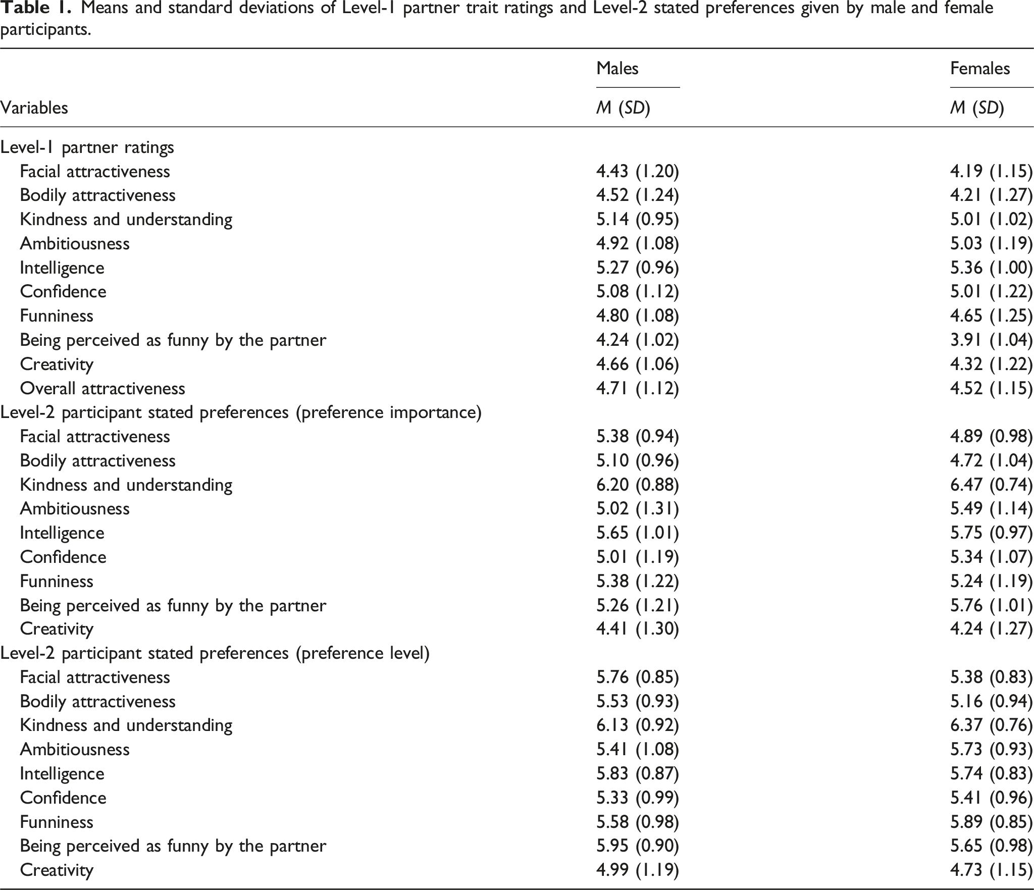
Means and standard deviations of Level-1 partner trait ratings and Level-2 stated preferences given by male and female participants.

Variables	Males	Females
	M (SD)	M (SD)
Level-1 partner ratings
Facial attractiveness	4.43 (1.20)	4.19 (1.15)
Bodily attractiveness	4.52 (1.24)	4.21 (1.27)
Kindness and understanding	5.14 (0.95)	5.01 (1.02)
Ambitiousness	4.92 (1.08)	5.03 (1.19)
Intelligence	5.27 (0.96)	5.36 (1.00)
Confidence	5.08 (1.12)	5.01 (1.22)
Funniness	4.80 (1.08)	4.65 (1.25)
Being perceived as funny by the partner	4.24 (1.02)	3.91 (1.04)
Creativity	4.66 (1.06)	4.32 (1.22)
Overall attractiveness	4.71 (1.12)	4.52 (1.15)
Level-2 participant stated preferences (preference importance)
Facial attractiveness	5.38 (0.94)	4.89 (0.98)
Bodily attractiveness	5.10 (0.96)	4.72 (1.04)
Kindness and understanding	6.20 (0.88)	6.47 (0.74)
Ambitiousness	5.02 (1.31)	5.49 (1.14)
Intelligence	5.65 (1.01)	5.75 (0.97)
Confidence	5.01 (1.19)	5.34 (1.07)
Funniness	5.38 (1.22)	5.24 (1.19)
Being perceived as funny by the partner	5.26 (1.21)	5.76 (1.01)
Creativity	4.41 (1.30)	4.24 (1.27)
Level-2 participant stated preferences (preference level)
Facial attractiveness	5.76 (0.85)	5.38 (0.83)
Bodily attractiveness	5.53 (0.93)	5.16 (0.94)
Kindness and understanding	6.13 (0.92)	6.37 (0.76)
Ambitiousness	5.41 (1.08)	5.73 (0.93)
Intelligence	5.83 (0.87)	5.74 (0.83)
Confidence	5.33 (0.99)	5.41 (0.96)
Funniness	5.58 (0.98)	5.89 (0.85)
Being perceived as funny by the partner	5.95 (0.90)	5.65 (0.98)
Creativity	4.99 (1.19)	4.73 (1.15)

Level metric

The relevant γ coefficients for the interaction between a stated preference and trait ratings on overall attractiveness – that is, the association between stated and revealed partner preferences (using preference importance) – are reported in Table 2. Here, we find general evidence for a correspondence between stated and revealed preferences when using the level metric. There were significant interactions detected for four out of the nine traits tested (kindness and understanding, intelligence, confidence, and creativity). For example, individuals who highly valued confidence were significantly more likely to give a higher overall attractiveness score to a partner they rated highly on confidence relative to individuals who valued confidence less.

Table 2.

Multilevel modelling coefficients(γ) for the association between stated and revealed preferences using stated importance for various traits. We note that each row of this table pertains to a separate model.

Stated preference $\times$ Partner ratings	Overall Attractiveness
	γ(SE)	95% CI	t	df	Sessions	n	p-value
Facial attractiveness	0.017(0.011)	[-0.005, 0.038]	1.551	884.33	171	1130	.1213
Bodily attractiveness	0.005 (0.012)	[-0.019, 0.029]	0.459	764.09	171	1132	.6466
Kindness and understanding	0.030 (0.015)	[0.001, 0.059]	1.983	670.71	171	1132	.0478
Ambitiousness	0.026 (0.015)	[-0.003, 0.055]	1.756	838.30	171	1131	.0795
Intelligence	0.036 (0.015)	[0.007, 0.065]	2.334	619.51	171	1132	.0199
Confidence	0.050 (0.018)	[0.015, 0.085]	2.829	439.30	123	753	.0049
Funniness	0.005 (0.022)	[-0.038, 0.048]	0.216	350.66	89	554	.8293
Perceived as funny	0.004 (0.024)	[-0.043, 0.051]	0.161	247.70	89	554	.8720
Creativity	0.050 (0.020)	[0.011, 0.089]	2.472	517.08	123	752	.0136

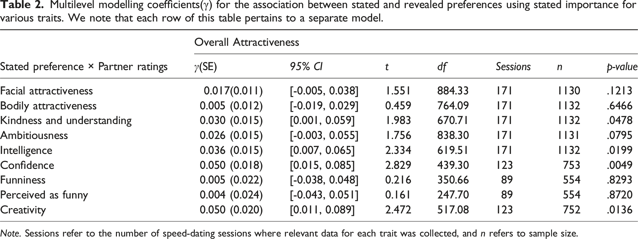
Note. Sessions refer to the number of speed-dating sessions where relevant data for each trait was collected, and n refers to sample size.

We conducted an additional analysis to investigate whether there was general evidence of a correspondence between stated and revealed preferences across all nine traits using the level metric (as opposed to performing nine separate level metric analyses). This involved restructuring the data so that preferences and trait ratings were nested under the traits they measured. We accounted for this nesting by introducing random intercepts and slopes for ratings and preferences grouped by trait. This allows us to simultaneously assess for the presence of a correspondence between stated and revealed preferences across the nine traits. Here, we found a significant interaction of preference importance on the association between trait ratings and overall attractiveness, meaning that we have general evidence for a correspondence between stated and revealed preferences (γ(SE) = 0.011(0.003), t(2248) = 3.220, p = .001).

Absolute difference

We investigated whether the absolute difference measure predicted ratings of overall attractiveness (Table 3). In all, the absolute difference between preference levels and trait ratings for facial attractiveness, intelligence and funniness were significantly associated with ratings of overall attractiveness. Again, we investigated whether there was an effect overall when we consider all traits at once while introducing relevant random intercepts and slopes (described previously for the level metric). We found that there was a significant association between the absolute difference between preferences and trait ratings and overall attractiveness (γ(SE) = −0.017(0.004), t(704.1) = −4.392, p < .001). That is, a higher discrepancy between a participant’s preference level and trait rating of their partner is associated with a lower rating of overall attractiveness. In sum, our analyses using two types of preferences demonstrate evidence of a correspondence between stated and revealed preferences using trait-by-trait measures.

Table 3.

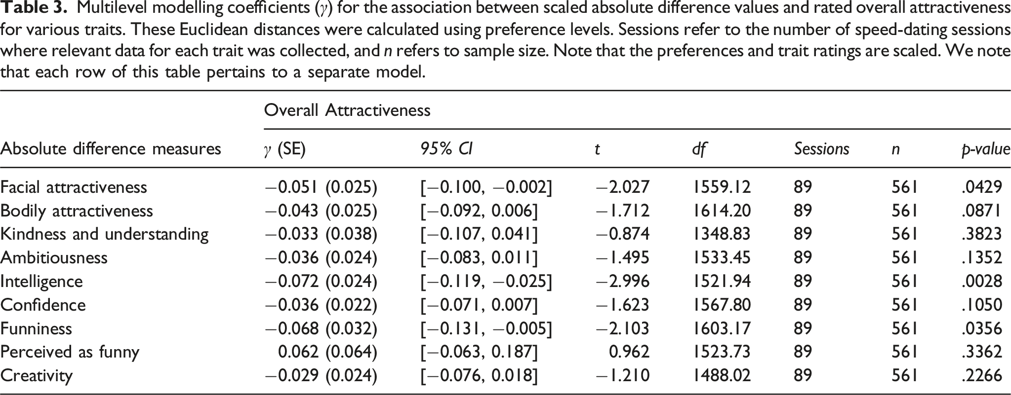
Multilevel modelling coefficients (γ) for the association between scaled absolute difference values and rated overall attractiveness for various traits. These Euclidean distances were calculated using preference levels. Sessions refer to the number of speed-dating sessions where relevant data for each trait was collected, and n refers to sample size. Note that the preferences and trait ratings are scaled. We note that each row of this table pertains to a separate model.

Absolute difference measures	Overall Attractiveness
	γ (SE)	95% CI	t	df	Sessions	n	p-value
Facial attractiveness	−0.051 (0.025)	[−0.100, −0.002]	−2.027	1559.12	89	561	.0429
Bodily attractiveness	−0.043 (0.025)	[−0.092, 0.006]	−1.712	1614.20	89	561	.0871
Kindness and understanding	−0.033 (0.038)	[−0.107, 0.041]	−0.874	1348.83	89	561	.3823
Ambitiousness	−0.036 (0.024)	[−0.083, 0.011]	−1.495	1533.45	89	561	.1352
Intelligence	−0.072 (0.024)	[−0.119, −0.025]	−2.996	1521.94	89	561	.0028
Confidence	−0.036 (0.022)	[−0.071, 0.007]	−1.623	1567.80	89	561	.1050
Funniness	−0.068 (0.032)	[−0.131, −0.005]	−2.103	1603.17	89	561	.0356
Perceived as funny	0.062 (0.064)	[−0.063, 0.187]	0.962	1523.73	89	561	.3362
Creativity	−0.029 (0.024)	[−0.076, 0.018]	−1.210	1488.02	89	561	.2266

In the General Introduction, we proposed that null results in past studies could also be attributed to the use of incongruent preference and analysis type, such as using preference levels with the level metric (e.g. Eastwick, Eagly, et al., 2011; Wu et al., 2018). We conducted additional analyses with such preference analysis and measure combinations to test these claims. When we use preference levels for the level metric, and preference importances for the absolute difference measure, both approaches yielded generally smaller effects ⁴ relative to their congruent counterparts (see Supplemental Materials). Given that the level metric and absolute difference measures make different assumptions about how preferences correspond to evaluations of overall attraction, it is feasible that null effects in past studies may have been attributed to a discordance between the preference type and measure type.

We acknowledge that our speed-dating sample is limited as it is not representative of the general population. A majority of our participants were first-year psychology students at a top Australian university, raising the likelihood that our sample was more intelligent and conscientious than the general population. This also meant that the age of the participants tended to be young on average, and we speculate that we may see stronger effects of stated preferences on revealed preferences in older participants who would be more serious and/or discerning about a potential romantic partner.

Although our sample size is large in absolute terms, one limitation of Study 1 was that we had a small number of participants of each sex (ranging from two to five) per speed-dating session. The small number of participants per speed-dating session may offset the power gains from a larger sample size because larger sessions with more speed-dating interactions yield more individual and partner variance that can be controlled via random intercepts due to the higher number of partner ratings for each individual. To assess the degree to which this issue affected our power, we ran additional simulations in which the sample size remained constant, but the number of males and females per session increased while the total number of sessions decreased (see Supplemental Materials). For the level metric, we found that the smaller number of participants per speed-dating session yielded somewhat less power than larger sessions with the same overall sample size. However, the size of our preference importance (n = 1145) and preference level samples (n = 561) still ensured considerably more statistical power compared to previous studies. We did not run additional simulations for the absolute difference method as we assumed the pattern of results would be similar.

Using a large sample, we find evidence that stated preferences exhibit some correspondence to attraction in a speed-dating context, though we obtain small effect sizes. While we identified that a mismatch between preference type and analysis method may contribute to the difficulty of detecting such a correspondence, this only occurs in a few studies (i.e. Eastwick, Eagly, et al., 2011; Wu et al., 2018). In Study 2, we propose a broader explanation for the limited correspondence seen here and in past studies.

Study 2: Trait-by-trait speed-dating simulations

Past studies have concluded that there may not be a correspondence between stated preferences and revealed preferences. Some have explained null results with the hot-to-cold empathy gap (Eastwick & Finkel, 2008) or construal theory (Trope et al., 2007; Trope & Liberman, 2003). Null effects have even been taken as evidence that stated preferences are invalid or meaningless (e.g. Campbell & Stanton, 2014; Eastwick et al., 2013). In Study 1, we found correspondences between stated and revealed preferences using the level metric and absolute difference analyses, which were likely detected thanks to large sample sizes.

Our findings still maintain the question of why the associations between stated and revealed preferences would be so small. One possible explanation is that humans vary across a number of dimensions and may use a large number of traits to romantically evaluate a potential partner. As the number of traits involved in partner evaluation increases, the relative contribution of each stated preference to the individual’s corresponding revealed preference decreases (Conroy-Beam & Buss, 2020).

The present study

Here, we use computer simulations to replicate the constraints and parameters of our speed-dating study and demonstrate how the association of stated preferences with revealed preferences decreases as the number of preferred traits increases. We closely replicate the design of our real-life speed-dating study so that direct comparisons can be made between the estimates obtained from simulated and real-life speed-dating data. This technique also allows for the exploration of ideas without being constrained by the practical limitations of data collection.

We conduct a set of simulations for each preference type because we make different assumptions regarding how overall attractiveness is calculated. For preference importance, we assume that the overall attractiveness of a potential partner is given by trait appeal. For preference level, we assume that the overall attractiveness of a potential partner is best approximated using Euclidean distance; a participant should perceive their partner as most attractive when a partner’s traits match a participant’s preference levels.

We simulate the conditions of the speed-dating sessions in Study 1 and empirically test the effects of changing: (1) the number of traits used to evaluate a potential partner, and (2) the extent to which stated preferences drive attraction to potential partners. When we define ratings of overall attraction to be completely driven by stated preferences, we can observe the maximum association that can be attained between stated and revealed preferences. In addition, we can estimate the power required to detect statistically significant associations between stated and revealed preferences under differing degrees to which attraction is driven by stated preferences. These analyses allow us to inform new interpretations of null findings in past studies.

Method

This simulation involves male and female participants rating opposite-sex partner attractiveness according to the constraints of the real-life speed-dating environment. The resulting data have been generated in the same structure as the real-life speed-dating data (see Figure 1) so that direct comparisons can be made between the γ obtained from simulated and real-life speed-dating data using multilevel modelling.

Figure 1.

Speed-dating simulation process. Note. 1) Generation of speed-dating interactions: Each participant is assigned partners to interact with in a speed-dating session. 2) Partner ratings: The participant rates the partner on traits 1 to n. The partner rating is a function of the partner’s latent trait value, the participant’s own biases, and some error. 3) Partner’s overall attractiveness score: The overall attractiveness score is calculated via trait appeal or Euclidean distance depending on the preference type. A variable amount of statistical noise is added to vary the extent to which a participant’s preference influences their overall evaluation of the partner. Each instance of noise is added for each trait. 4) The same process from 1) to 3) is repeated for the remaining partners.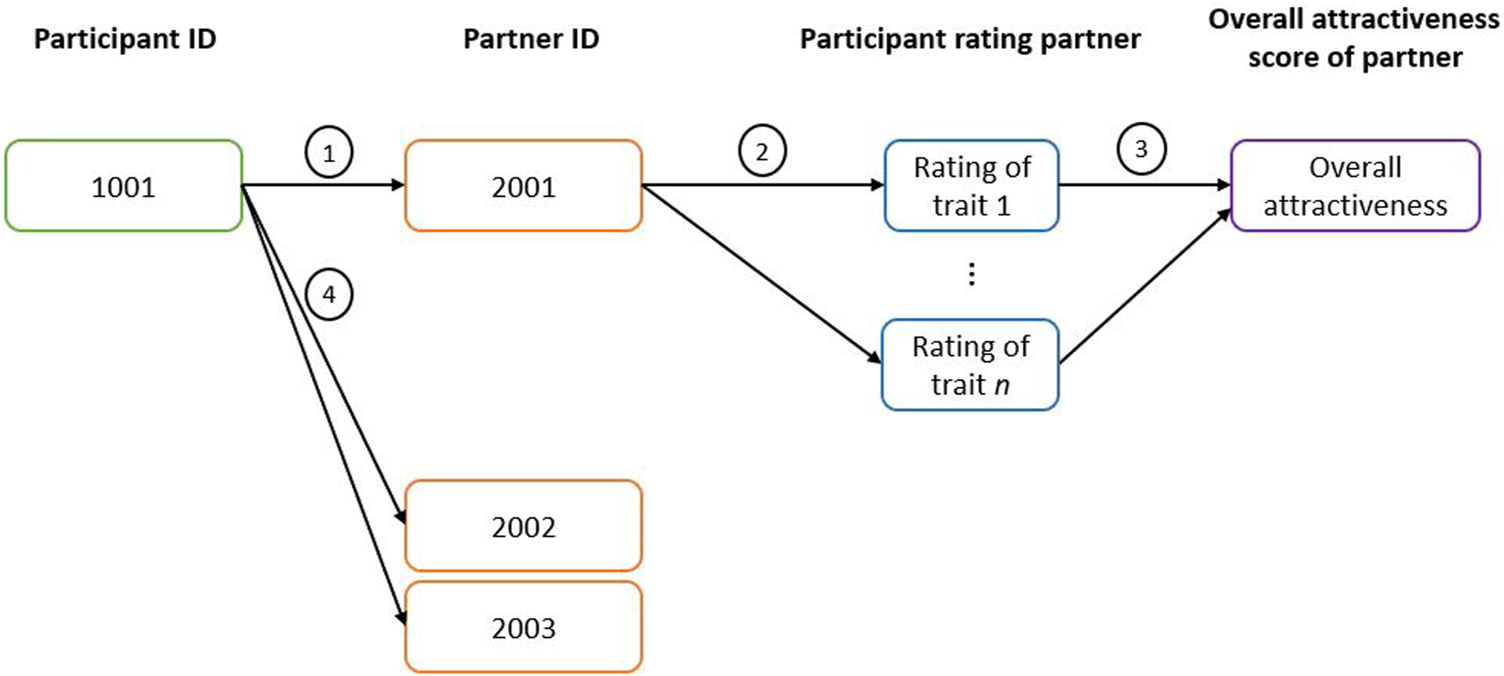

Variable definitions

Participant _i

Denotes the specific individual who gives the rating within the simulation, this is given by their ID number (1000, 1001, …).

Partner _j

Denotes another participant j who receives trait, trait appeal, and overall attractiveness ratings by participant i, this is given by their ID number (1000, 1001, …).

Trait _k

Denotes the kth trait, where k ranges from 1 to n (the maximum number of traits used to determine overall attractiveness in the simulation). Examples of traits may be facial attractiveness, intelligence, confidence, etc. It is assumed that all traits are independent of one another.

Latent trait score _jk

The extent to which partner j possesses a certain trait k on a scale from 1 = Well below average to 7 = Well above average. Each participant’s latent trait value has been sampled from a normal distribution (M = 4.00, SD = 1.50).

Stated trait preference _ik

Preference importance is defined as the extent that participant i believes it is important for an ideal partner to possess trait k. Preference level is participant i’s preferred level of a trait k possessed by an ideal partner. Each participant’s stated preference value has been sampled from a normal distribution (M = 4.00, SD = 1.50), where values were rounded and ranged from 1 to 7. We note that we generate preference importances and levels in the same way.

Rating bias _i

Each participant i may exhibit a systematic tendency to over or underestimate their rating of their partners’ traits. This bias has been sampled from a normal distribution (M = 0.00, SD = 1.50) and will add variation to each participant’s trait ratings.

Parameters

The simulation has several parameters that may be changed to suit different scenarios:

• The number of traits used by each participant to determine overall attractiveness, varying from 2 to 25.

• The number of speed-dating sessions within each simulation.

o For simulations regarding the level metric, there were 171 speed-dating sessions, as per the maximum number of sessions in the real-life speed-dating data which measured preference importances (see Table 2).

o For simulations regarding the absolute difference method, there were 89 speed-dating sessions which measured preference levels (see Table 3)

• The number of males and females per session was generated according to a normal distribution, rounded to the nearest integer, and restricted between 2 and 5 as per the real-life speed-dating data. For the level metric, males: M = 3.582, SD = 0.902, and females: M = 3.693, SD = 0.839. For the absolute difference measure, M = 3.157, SD = 0.732, females: M = 3.433, SD = 0.641.

• A noise term is the magnification of the random error included in the calculation of overall attractiveness. We only manipulate noise here, so that we can directly manipulate the extent that preference-trait rating combinations have on the judgement of overall attractiveness. For each preference-trait rating combination, random error (M = 0, SD = 1) is multiplied by the noise term ranging from 0 to 50. A noise value of 0 would mean that stated preferences were perfectly measured and completely drove attraction to a partner depending on their traits. A higher noise value corresponds to a simulation in which there is a decreased degree of participants acting in accordance with their stated preferences.

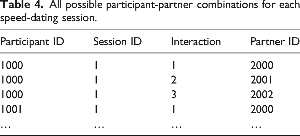
Generation of speed-dating interactions

The number of males and females per speed-dating session was generated according to parameters obtained from the real speed-dating data. Participant IDs were generated for each individual where males had IDs starting from 1000 and female IDs starting from 2000. Combinations for each participant and partner were generated for each session and ‘Interaction’ is the order in which a participant meets their partner (see Table 4).

Table 4.

All possible participant-partner combinations for each speed-dating session.

Participant ID	Session ID	Interaction	Partner ID
1000	1	1	2000
1000	1	2	2001
1000	1	3	2002
1001	1	1	2000
…	…	…	…

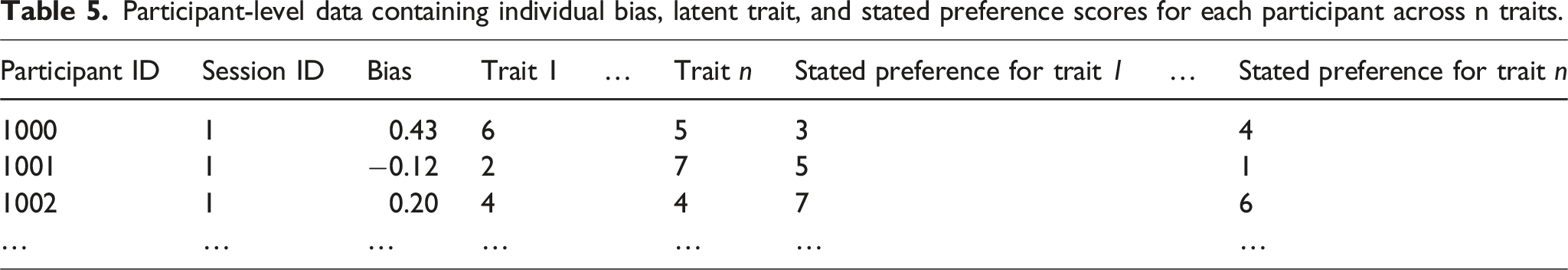
Assigning participant traits

Each participant was assigned latent trait scores, a rating bias, and stated preferences. Latent trait scores and stated preferences were generated for the specified number of traits according to the distribution of preferences from the speed-dating data and rounded to the nearest integer between 1 and 7. A rating bias was then generated for each individual. These resulted in a table of Level-2 data (see Table 5).

Table 5.

Participant-level data containing individual bias, latent trait, and stated preference scores for each participant across n traits.

Participant ID	Session ID	Bias	Trait 1	…	Trait n	Stated preference for trait 1	…	Stated preference for trait n
1000	1	0.43	6		5	3		4
1001	1	−0.12	2		7	5		1
1002	1	0.20	4		4	7		6
…	…	…	…		…	…		…

Partner ratings

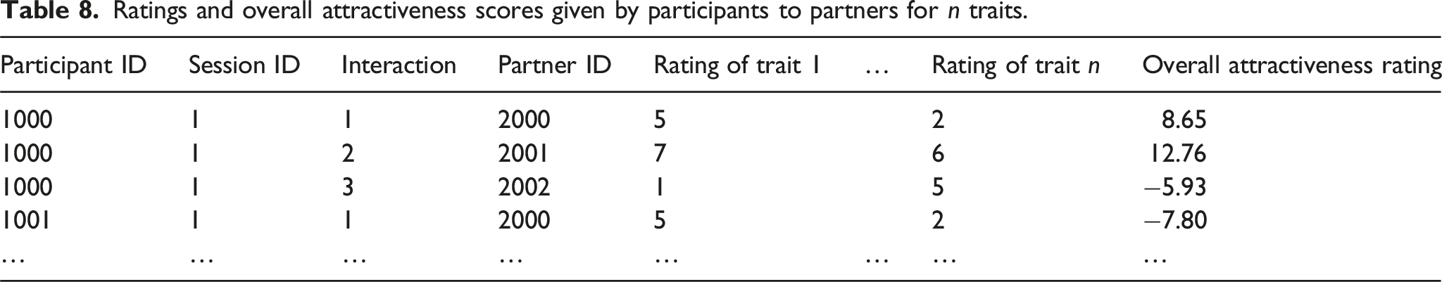
The data from Table 4 and Table 5 were combined to create a data-frame for partner ratings (Level-1). This data-frame was filled with participants’ ratings of their partners. Participant i’s rating for partner j’s kth trait was a function of the partner’s latent score for trait k, the participant i’s rating bias, and a normally distributed error term (M = 0.00, SD = 1.00) to mimic rating variability across partners.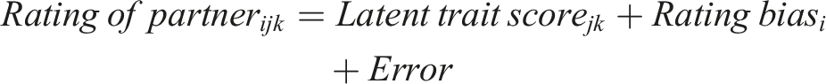

$Rating\hspace{0.17em}of\hspace{0.17em}{partner}_{ijk}=Latent\hspace{0.17em}trait\hspace{0.17em}{score}_{jk}+Rating\hspace{0.17em}{bias}_i+Error$

The partner rating was rounded to the nearest integer between 1 and 7 as per the real-life speed-dating data.

Calculation of overall attractiveness using preference importance

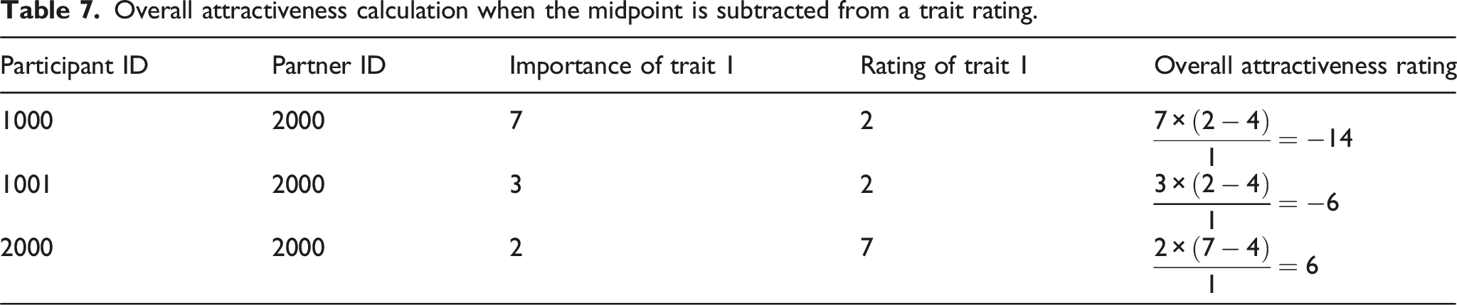
Similar to the level metric, we assume that the higher a participant’s preference importance for a trait, the more appealing a partner becomes when they possess that trait. Here, we assume that overall attractiveness is estimated using trait appeal. The trait appeal score is the extent to which partner j’s kth trait is attractive to participant i, given by the participant’s preference importance for the trait multiplied by the participant’s rating of the partner on the trait minus the midpoint (i.e. 4). These weighted values are then averaged by the number of traits considered.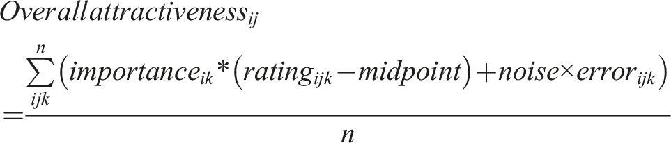

${Overall\hspace{0.17em}attractiveness}_{ij}=\frac{{\displaystyle \sum }_{ijk}^n\left({importance}_{ik}*\left({rating}_{ijk}-midpoint\right)+noise\times {error}_{ijk}\right)}{n}$

The reason for this latter subtraction is that we assume high ratings on these traits are universally valued. A trait rating below the scale midpoint (‘average’) (See Study 1 Materials) detracts from a potential partner’s appeal, conversely, a trait rating above the midpoint adds to their appeal (the extent to which this occurs is proportional to the importance of the trait). We do not make the same adjustment for preference importance as there is no midpoint, and the traits in question are universally desirable, therefore any importance assigned to these traits can be treated as a positive weight for the calculation of trait appeal.

Consider the following scenario (Table 6): If we did not subtract the midpoint, an individual who greatly valued a certain trait (e.g. 7) who was evaluating a potential partner that was well below average on that trait (e.g. 2) would find the same potential partner more appealing than someone who valued the trait less (e.g. 3) – which does not make sense. It would also be odd that a partner could be equally appealing compared to the former if an individual did not value a trait to a large extent (e.g. 2), but the partner scored highly on the corresponding trait (e.g. 7). We would expect that an individual’s attraction to their partner would diminish due to their partner falling below average on an important trait, whereas a participant’s attraction to a partner should increase (to a lesser extent) on a trait that is less important if the partner is rated above average for that trait. We adjust for this by subtracting the midpoint (Table 7).

Table 6.

Overall attractiveness calculation when the midpoint is not subtracted from a trait rating.

Participant ID	Partner ID	Importance of trait 1	Rating of trait 1	Overall attractiveness rating
1000	2000	7	2	$\frac{7\times 2}{1}=14$
1001	2000	3	2	$\frac{3\times 2}{1}=6$
2000	1000	2	7	$\frac{2\times 7}{1}=14$

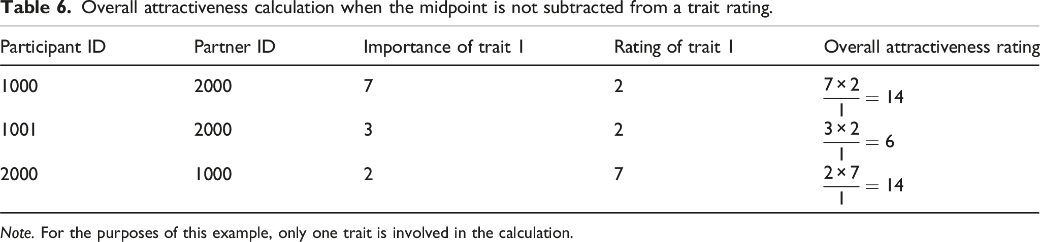
Note. For the purposes of this example, only one trait is involved in the calculation.

Table 7.

Overall attractiveness calculation when the midpoint is subtracted from a trait rating.

Participant ID	Partner ID	Importance of trait 1	Rating of trait 1	Overall attractiveness rating
1000	2000	7	2	$\frac{7\times \left(2-4\right)}{1}=-14$
1001	2000	3	2	$\frac{3\times \left(2-4\right)}{1}=-6$
2000	2000	2	7	$\frac{2\times \left(7-4\right)}{1}=6$

We then added a noise term to vary the extent to which a participant ‘acts’ in accordance with their stated preferences. This term is a multiplier that varies the amount of normally distributed random error (M = 0.00, SD = 1.00) added in the calculation of overall attractiveness (estimated via trait appeal) (note: an error term is generated for each speed-dating interaction). When noise is 0, there is no error, and trait appeal is purely the product of the partner trait rating and the stated preference for a particular trait. The overall attractiveness rating is given by this trait appeal score (Table 8). We average across the traits so that the resulting value is not biased by the number of traits involved in the simulation.

${Overall\hspace{0.17em}attractiveness}_{ij}=\frac{{\displaystyle \sum }_{ijk}^n\left({importance}_{ik}*\left({rating}_{ijk}-midpoint\right)+noise\times {error}_{ijk}\right)}{n}$

Table 8.

Ratings and overall attractiveness scores given by participants to partners for n traits.

Participant ID	Session ID	Interaction	Partner ID	Rating of trait 1	…	Rating of trait n	Overall attractiveness rating
1000	1	1	2000	5		2	8.65
1000	1	2	2001	7		6	12.76
1000	1	3	2002	1		5	−5.93
1001	1	1	2000	5		2	−7.80
…	…	…	…	…	…	…	…

Calculation of overall attractiveness using preference level

When using preference levels and the absolute difference measure, we assume that overall attractiveness is best modelled using the Euclidean distance, where a partner should be maximally attractive when a partner’s trait ratings match an individual’s preference levels. The following formula describes the Euclidean distance calculation for each interaction between participant i and partner j where n is the total number of traits, and k is the kth trait. We also added a noise term to vary the extent to which a participant ‘acts’ in accordance with their stated preferences. This term is a multiplier that varies the amount of normally distributed random error (M = 0.00, SD = 1.00) added in the calculation of overall attractiveness (estimated via Euclidean distance) (note: an error term is generated for each preference-trait rating pair). Given that Euclidean distance indicates a multidimensional discrepancy between preferences and trait ratings, when calculating our overall attractiveness rating, the Euclidean distance was multiplied by −1 so that a lower Euclidean distance score indicated higher attractiveness.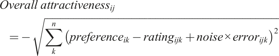

${Overall\hspace{0.17em}attractiveness}_{ij}=-\hspace{0.17em}\sqrt{{\displaystyle \sum }_k^n{\left({preference}_{ik}-{rating}_{ijk}+noise\times {error}_{ijk}\right)}^2}$

Calculation of the predictive validity of stated preferences

The same level composition was used as per Study 1. We used multilevel modelling to investigate the extent that preference importances are associated with revealed preferences when using the level metric and preference importance responses; or in the case of preference level, the extent to which the absolute difference between a preference level and trait rating is associated with overall attractiveness; given by γ. For each simulation, we conduct one analysis using the preference and trait rating for Trait 1, with the dependent variable being overall attractiveness. We do this because the traits were independently generated with no distinguishing characteristics between them. We assume that the results of one analysis regarding Trait 1 are representative of the results for traits up to Trait n.

Results and discussion

Level metric

The simulation was run with 171 sessions to replicate the maximum number of sessions available from the real speed-dating data for which we had preference importance responses. We initially simulated a scenario where overall attractiveness ratings were completely driven by participants’ stated preferences and their partners’ traits – that is, the noise term was set to 0. Figure 2 shows the effect of the number of traits used to judge the overall attractiveness of a partner, and the interaction term γ, which is a measure of the relationship between stated and revealed preferences for a given trait.

Figure 2.

Results of a simulation where overall attractiveness ratings were completely driven by participants’ (on average, n = 1244) stated preferences and their partners’ traits. Note. This was implemented by setting the noise term to 0 and the number of traits to 2, 3, 5, 9 (the number of preferences measured in our real speed dating data), 10, 15, 20, and 25. The simulation was run 1000 times per trait parameter. The extent to which the stated preference for one trait was associated with the revealed preference for the same trait is given by the interaction estimate γ. The black points indicate the estimate from each simulation and the trendline is given by a Loess regression line.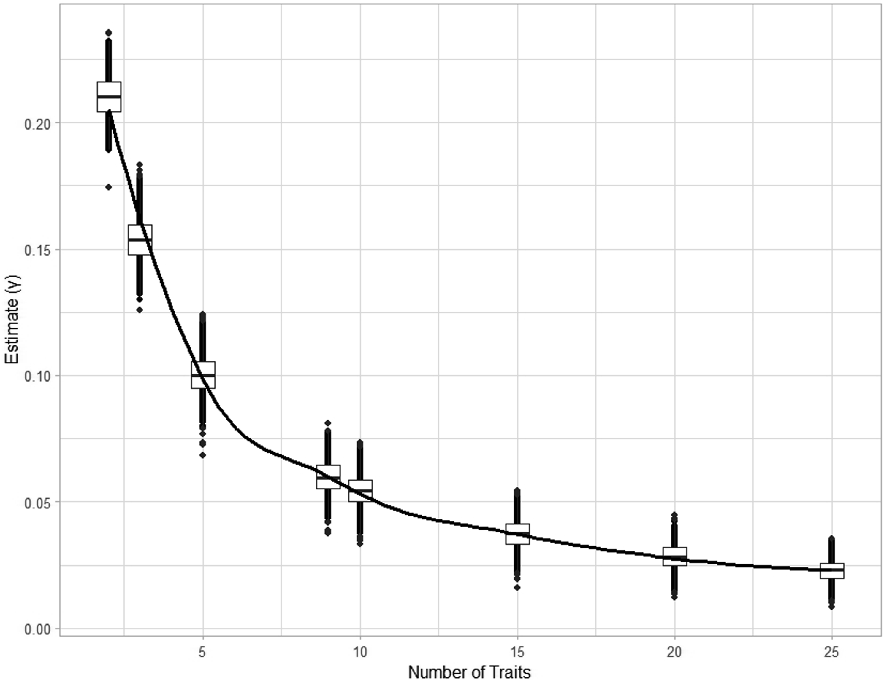

Figure 2 shows that even when participants behave entirely in accordance with their stated preferences, the magnitude of the interaction effects is not necessarily substantial. We obtain a maximum median interaction estimate of γ = 0.210 when participants only use two traits to judge overall attractiveness. As the number of traits increase, γ continues to decrease, reaching γ = 0.023 at 25 traits. For reference, the largest γ in Study 1 was 0.050. To better visualise the effect of interaction size, Figure 3 shows an interaction plot which demonstrates the maximum interaction estimate γ = 0.210. For every 1 standard deviation increase in preferences, the slope coefficient between trait rating and overall attractiveness additionally increases by 0.210. We note that an interaction estimate of γ = 0 would be represented by parallel lines in the same plot, indicating no correspondence between stated and revealed preferences.

Figure 3.

Example of an interaction plot indicating the effect of an interaction estimate γ = 0.210 (the interaction estimate when two preferences completely drive attractiveness ratings) across varying preference values. Note. Preferences, trait ratings, and overall attractiveness ratings have been scaled such that the mean is 0 and standard deviation is 1. Main effects used to plot this figure were obtained from a single simulation and may vary across simulations.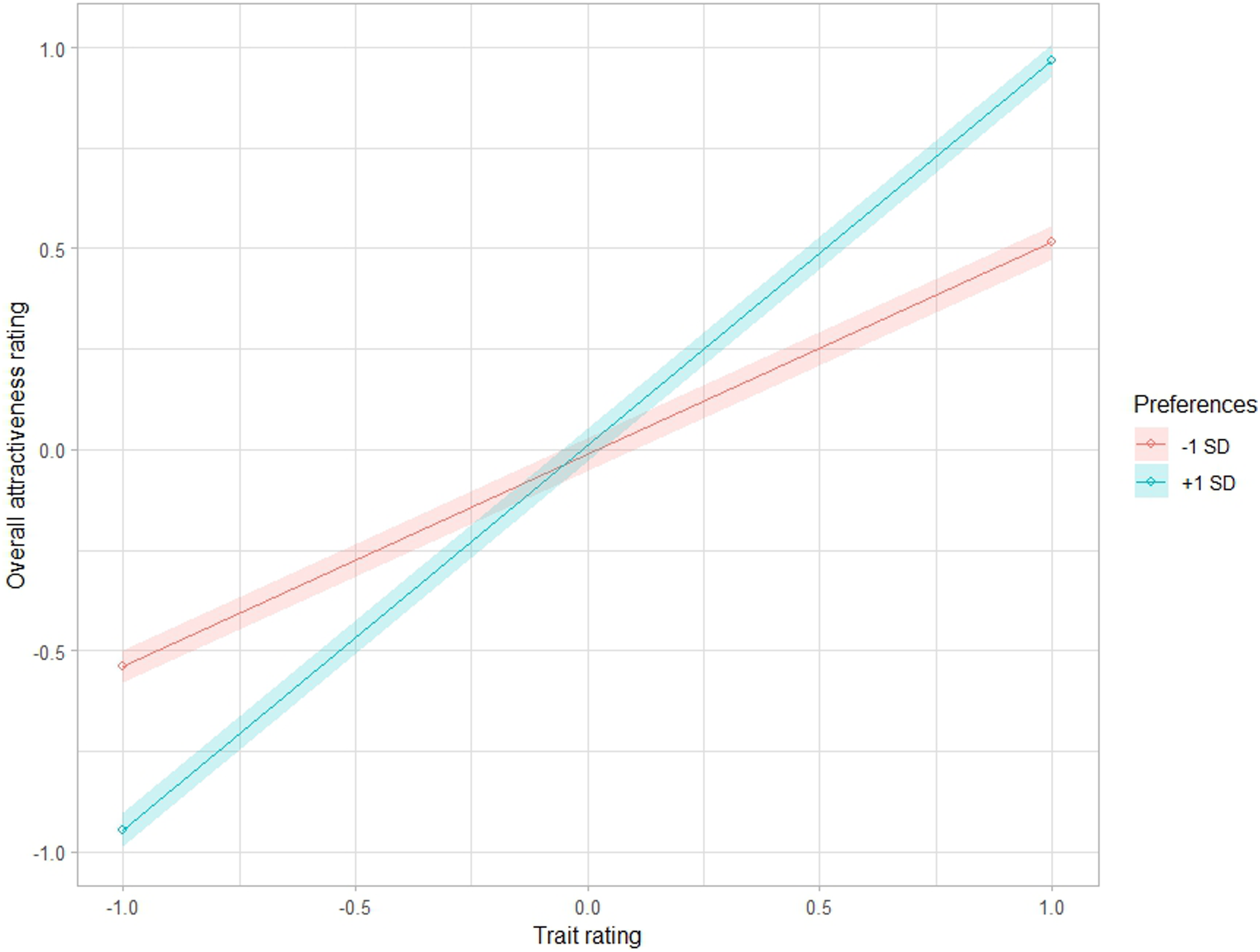

Again, Figure 2 demonstrates a scenario where participants act entirely in accordance with their stated preferences. A more realistic scenario is that individuals’ actions are influenced, but not completely driven by their stated preferences. We created several models to investigate the effect of changing the extent to which an individual’s revealed preferences are driven by their stated preferences (see Figure 4).

Figure 4.

Varying the number of traits (2, 3, 5, 9, 10, 15, 20, and 25) and the amount of noise on the size of the interaction effect between stated preferences, and trait ratings on overall attractiveness. Note. A noise term of 0 is the scenario where stated preferences are perfectly measured and participants (on average n = 1244) behave entirely in accordance with their stated preferences, i.e. where 100% of the variance of trait appeal scores is accounted for by stated preferences. Noise is the magnification of the random error included in each trait appeal score. Noise values 5, 10, 20, 30, 40, and 50 correspond to (on average) 91%, 72%, 39%, 22%, 14%, and 10%, respectively, of the percentage variance shared with trait appeal with noise = 0 when there are 9 traits involved. That is, a higher noise value corresponds to a simulation in which there is a decreased correspondence between participants acting in accordance with their stated preferences.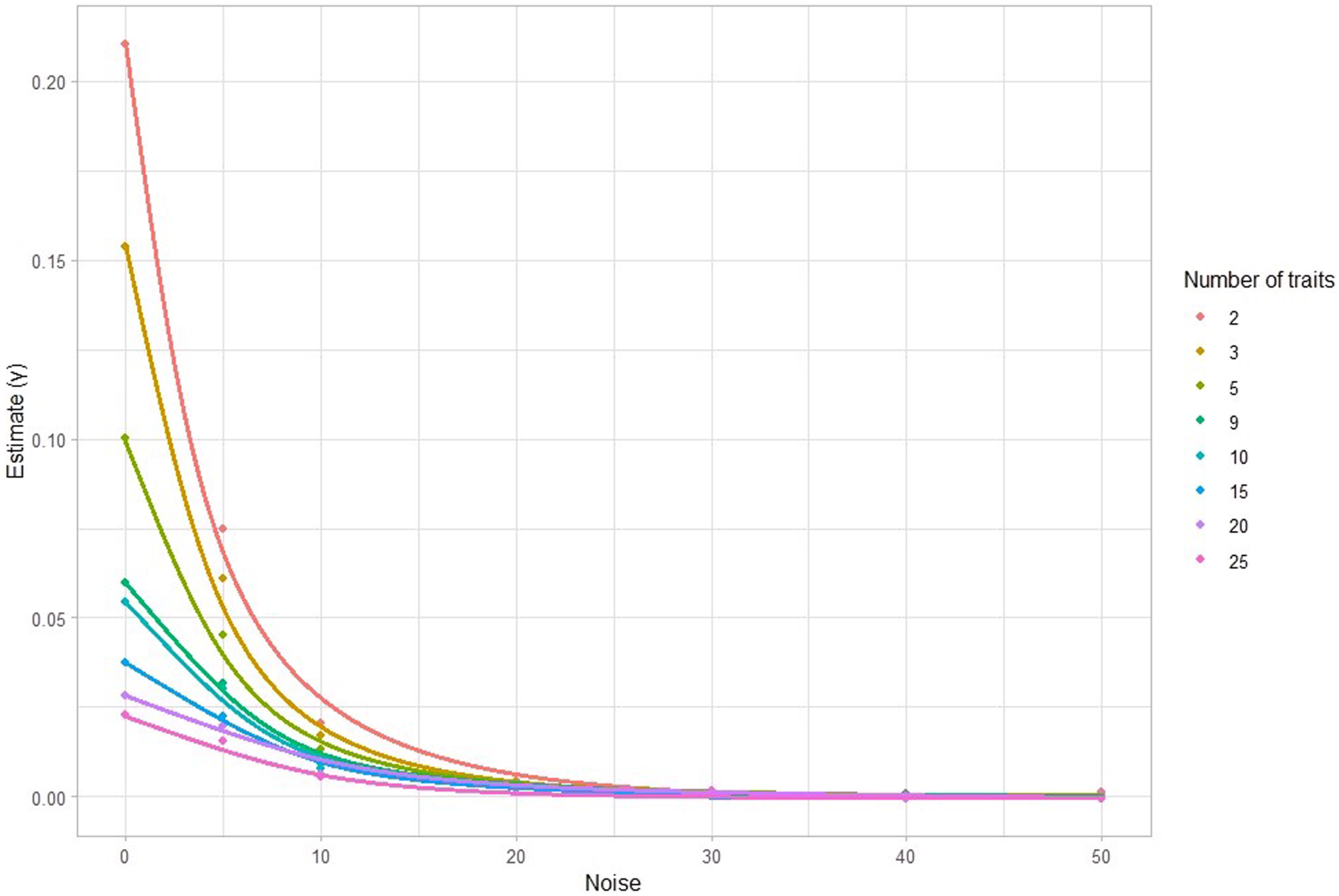

Figure 4 shows how increasing noise decreases γ. The shape of each trendline depends on how many trait preferences are involved in attraction, but in general, it can be seen that when noise is substantial and when there are more than a few traits involved, effects are very small.

The proportion of significant γ estimates for each set of 1000 simulations has been calculated to estimate statistical power – the probability of obtaining a significant estimate given that a true effect exists (α = .05) (Figure 5). Across all the trait numbers tested, as noise increased, the proportion of significant estimates detected decreased. When 9 traits influenced the evaluation of overall attraction (as per the real-life speed-dating data), noise terms of 0, 5, 10, 20, 30, 40, and 50 corresponded to the following proportion of estimates detected to be significant 1.000, .573, .099, .055, .064, .047, and .041, respectively.

Figure 5.

The effect of varying the number of traits and the amount of noise on the power of detecting a significant relationship between stated and revealed preferences (on average, n = 1244).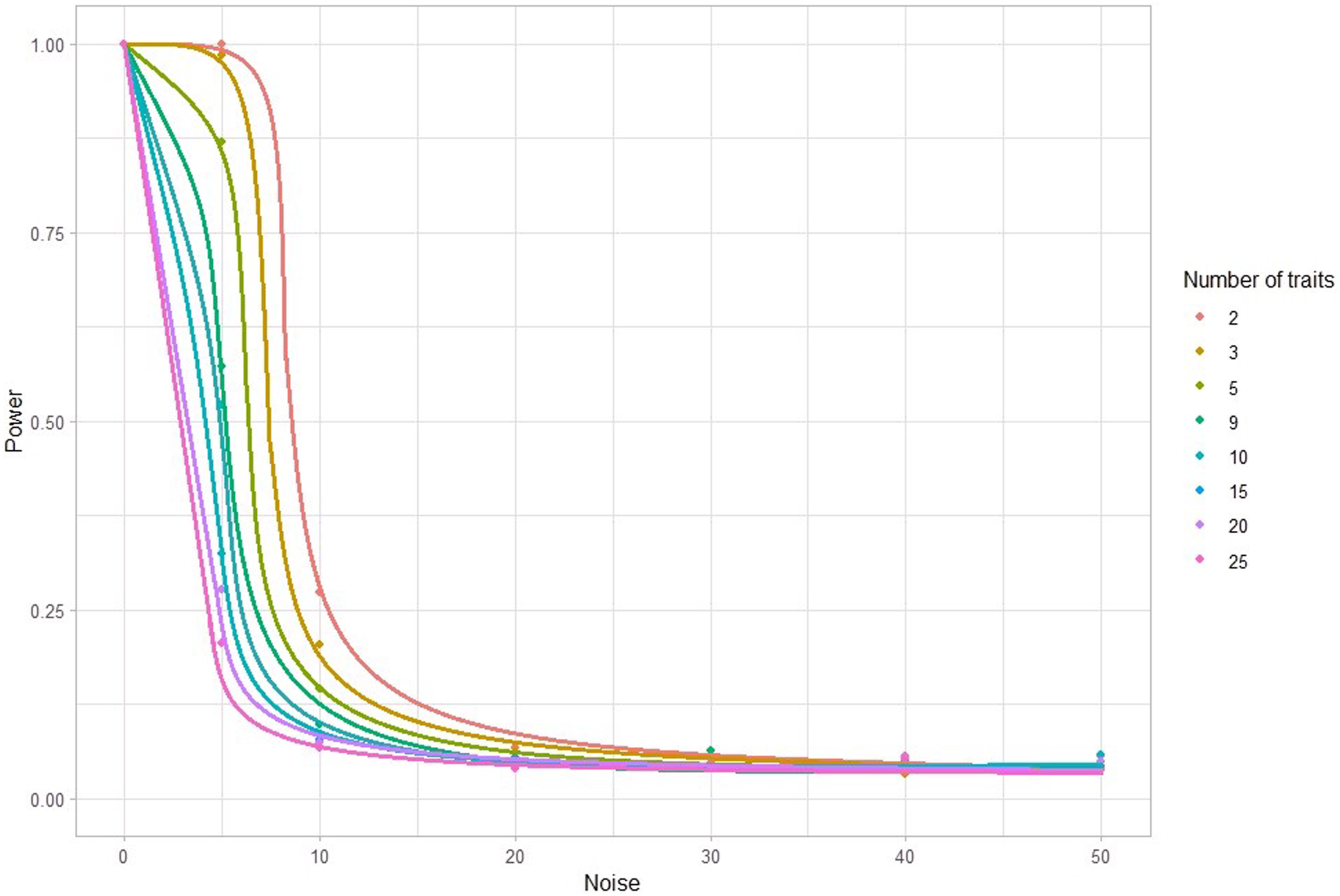

In a real-life speed-date, it is likely that participant behaviours are not completely driven by their stated preferences. Factors such as measurement error or other extraneous variables within the study are likely to contribute to error. This has been modelled in the simulation where we demonstrate that noise dramatically decreases both the magnitude of γ and the power to detect a significant γ (Figures 4 and 5). And when factors such as mate-attraction complexity (i.e. the number of traits involved in judging a partner’s overall attractiveness) are taken into consideration, we see a more dramatic decrease in the magnitude of γ and power.

Absolute difference

The simulation was run with 89 sessions to replicate the maximum number of sessions available from the real speed-dating data for which we had preference level responses. We found that as the number of traits used to judge the overall attractiveness of a partner increased, the size of the effect γ, as well as power decreased. We also see this is the case across all noise values, where increasing noise further decreases the effect size and power (see Supplemental Materials for full figures).

Study 3: Omnibus measures

From Studies 1 and 2, it becomes apparent that the lack of correspondence between stated and revealed preferences may not be due to an absence of an effect but could be attributed to an exclusive focus on individual trait-by-trait analyses. Examining traits in isolation does not reflect the real-life multivariate way in which individuals evaluate other potential partners (Lee et al., 2014). In Study 3, we investigate commonly used omnibus measures that allow us to explore the combined impact of multiple mate preferences on overall partner evaluation. As mentioned in the General Introduction: Omnibus Measures, the implicit assumptions of omnibus measures are seldom considered in past applications. Here, we discuss and evaluate various omnibus measures, and identify problems that may arise from their use.

Considerations regarding omnibus measures

When we find a significant association between an omnibus measure and a romantic outcome (e.g. rating of overall attractiveness), we assume that this indicates a correspondence between stated and revealed preferences. Specifically, a correspondence would imply the congruent combination of preference-trait rating pairs (e.g. stated preferences for intelligence paired with partner ratings of intelligence, and so on). Here, we consider the possibility that the observed association could arise as an artefact, independent of a true correspondence between stated and revealed preferences ⁵ . We investigate whether the results of various omnibus tests do indeed reflect a specific preference-trait rating correspondence.

The present study

We aim to investigate whether stated preferences correspond to revealed preferences using various omnibus measures. We evaluate whether the (raw and corrected) pattern metric, Euclidean distance, and trait appeal are associated with ratings of overall attractiveness in our speed-dating sample. Expanding on Study 2, we also use simulations to investigate how the number of traits involved in partner judgement influences the effect size and power to detect a correspondence between stated and revealed preferences using omnibus measures.

Previous studies have identified that omnibus measures may be more likely to encounter Type I errors due to limitations such as the normative desirability bias. Here, we explore a bias that has not been identified in the past. When we use any omnibus test, we assume that a positive association between an omnibus measure and overall attractiveness can be attributed to the congruent combination of preference-trait rating pairs (e.g. stated preferences for intelligence and ratings of potential partners’ intelligence and so on). We test this assumption with the novel use of permutation tests; these tests estimate the probability that a correspondence observed in our speed-dating data could be obtained through a random combination of preference-trait rating pairs (e.g. preference for intelligence paired with ratings of facial attractiveness). Permutation tests offer the advantage of maintaining the exact distribution of measured preferences and trait ratings, unlike simulation techniques that sample from an approximate distribution of the observed data.

Expanding on Study 2, we use simulations to investigate how the number of traits involved in partner judgement influences the effect size and power to detect a correspondence between stated and revealed preferences. We specifically estimate overall attractiveness using a large number of traits (i.e. 25) and investigate the effect of varying the number of traits used to calculate our omnibus measures. Conroy-Beam and Buss (2020) similarly investigated mate-attraction complexity, calculating preference fulfilment (average Euclidean distance across each participant’s interactions) and predictive power (average correlation between each preference and partner trait), but they did not investigate the association between these measures and a romantic outcome (Eastwick et al., 2019). In addition, no studies to date have explored the role of mate-attraction complexity using other omnibus measures such as the (raw and corrected) pattern metric or trait appeal. Further, we evaluate and critique the viability of omnibus measures in light of our findings and extant literature.

Methods

Speed-dating data analyses

Stated preferences (both preference importance and level), trait ratings, and overall attractiveness were measured as per Study 1.

Pattern metric

We excluded speed-dating interactions if they were missing any responses to the preference level or rating items, resulting in 561 participants included in this analysis. We calculated the raw pattern metric score by calculating Pearson’s r correlations for each speed-dating interaction, and mean-centred each individual’s preferences and trait ratings prior to the Pearson’s r correlations for the corrected pattern metric. The resulting pattern metric values (Pearson’s r) were then scaled (such that M = 0, and SD = 1) prior to analysis.

Contrary to Eastwick et al. (2019) and Fletcher et al. (2020), who apply a Fisher Z-transform of the obtained r values to ensure the normal distribution of the resulting pattern metric scores, we did not perform this transformation for several reasons. First, the r values obtained were roughly normal (see Supplemental Materials). Second, the Fisher Z-transform is undefined when r = −1 or r = 1, which would result in the unnecessary exclusion of 16 valid observations when using preference importances.

Euclidean distance

The omnibus Euclidean distance was calculated as per Study 2. As it is not appropriate to compare Euclidean distances calculated using different dimensions (i.e. different numbers of traits), we excluded speed-dating interactions if they were missing any responses to the preference level or trait rating items, resulting in 561 participants in this analysis. A Euclidean distance was calculated for each speed-dating interaction between participant i and partner j across each kth trait, for n = 9 traits. The resulting Euclidean distance values were scaled prior to analysis.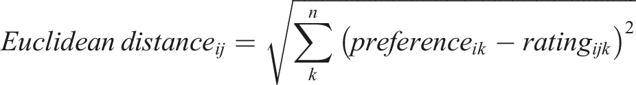

${Euclidean\hspace{0.17em}distance}_{ij}=\sqrt{{\displaystyle \sum }_k^n{\left({preference}_{ik}-{rating}_{ijk}\right)}^2}$

We do not control for the normative desirability bias as it does not make sense to mean-centre preference level responses and trait ratings before calculating the difference between these two values. The preference levels and trait ratings are assessed on the same scale (1 = Well below average, 7 = Well above average), so mean-centring responses would shift the relative scales of responses. The intended purpose of using a Euclidean distance measure is to model how a potential partner is optimally attractive when preference levels are satisfied. Since the participant would have no knowledge or awareness of what the mean-centred ratings would be, it would not make sense that overall attractiveness is optimised when the mean-centred preference matches the mean-centred trait rating.

Trait appeal

Trait appeal was calculated for each speed-dating interaction between participant i and partner j across each kth trait, for n = 9 traits. Only the data from 2017–2019 were used where we had a complete set of nine preference importances and trait ratings (n = 561). The resulting trait appeal values were scaled prior to analysis.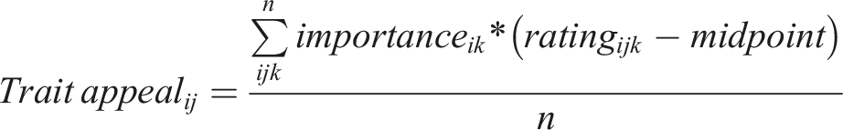

${Trait\hspace{0.17em}appeal}_{ij}=\frac{{\displaystyle \sum }_{ijk}^n{importance}_{ik}*\left({rating}_{ijk}-midpoint\right)}{n}$

Speed-dating simulations

We explore how the number of traits considered in the evaluation of a speed-dating partner in an omnibus measure affects the effect size and power to detect an association between our omnibus measures and overall attractiveness in a simulation. We also accounted for the conceptual difference between preference importance and preference, by using different measures to approximate overall attractiveness for different preference types. Similar to Study 2, we use trait appeal to estimate the overall attractiveness score in simulations where preference importances are generated, and we use Euclidean distance to estimate the attractiveness in simulations where preference levels are generated. However, the number of traits used to calculate overall attractiveness was constant, where we assume that overall attractiveness is judged on a large number of traits (i.e. 25 traits). For simulations involving preference importance, we calculated trait appeal, as well as both the raw and corrected pattern metric. And for simulations using preference level, we calculated both pattern metrics and the Euclidean distance.

Multilevel modelling was used to calculate the association between each omnibus measure and overall attractiveness, given by γ. We calculated trait appeal and Euclidean distance across 2, 3, 5, 9, 10, 15, 20, and 25 traits. For the pattern metric, we performed simulations for 3 or more traits; calculating Pearson’s correlation coefficient between any two observations will always result in r equal to 1 or -1, which would not be meaningful. We varied the amount of noise for the pattern metric, Euclidean distance, and trait appeal simulations. We used noise parameters 0, 5, 10, 20, 30, 40, and 50 for the pattern metric, but we used a noise value of 1 instead of 0 for the Euclidean distance and trait appeal simulations due to singularities between the omnibus measure and the overall attractiveness value (the omnibus measure we are analysing is the same measure used to approximate overall attractiveness).

Permutation test

Given that omnibus measures combine multiple preferences and trait ratings, it is essential to determine if the observed effect is a genuine reflection of a unique connection between preferences and trait rating pairs or whether these observed effects are spurious (e.g. due to some unforeseen bias). To quantify the extent to which individual preferences are meaningful in these omnibus measures, we conducted permutation tests for each measure.

A permutation test does not require assumptions about the distribution of the data and only requires that each simulation is independent and identically distributed under the null hypothesis (Fisher, 1935). A permutation test estimates the p-value of obtaining our observed effect (in the real data) by shuffling stated preferences across traits while keeping other variables constant. Here, we repeatedly simulate the scenario where preferences have no actual correspondence to trait ratings. The p-value is the estimated probability of obtaining an association (between the omnibus measure and overall attractiveness) as extreme or more extreme than what is obtained in the real speed-dating data (Fisher, 1935). A low p-value suggests that the observed result in the speed-dating data was unlikely to have occurred by chance, reinforcing the meaningfulness of the specific preference-trait rating pairs. Conversely, a high p-value suggests that the result was likely to have occurred by the chance combination of trait ratings and their preferences.

We carried out 50,000 simulations for each of the omnibus measures. For each simulation, numbers from 1 to 9 were selected randomly and without replacement (because we have 9 traits). The resulting sequence of numbers represented the new order of preferences (with the order of the original preferences being 1, 2, … 9). Preference order was randomised once for each simulation. Within each simulation, the same order of preferences was applied for all participants such that the distribution of each preference was not affected. The same omnibus measures and multilevel modelling analysis were then conducted on the randomised data (See Supplemental Materials for example). The p-value was estimated by counting the number of instances in which we obtained a t-statistic as extreme or more extreme than the one obtained in the real speed-dating data and then dividing this number by the total number of simulations (50,000).

Results

Pattern metric

Using preference levels, both the raw and corrected pattern metric were associated with overall attractiveness (γ(SE) = 0.049(0.023), t(1494.65) = 2.118, p = .034, and γ(SE) = 0.079(0.021), t(1501.46) = 3.719, p < .001, respectively). When we conducted the permutation test for the raw pattern metric, we obtained a t-statistic as extreme or more extreme than our result obtained from the real speed-dating data with a probability of .314, indicating that the association between the raw pattern metric and overall attractiveness in the speed-dating data is spurious and were likely to have been observed even if discordant preferences and trait ratings were used in the calculation of the raw pattern metric. Performing the permutation test on the corrected pattern metric, we obtained an estimated p-value of .002, indicating that it is likely that the corrected pattern metric’s association with overall attractiveness could indeed depend on the concordance between preferences and trait ratings.

Using preference importances instead of preference levels, the raw pattern metric did not predict overall attractiveness, but the corrected pattern did (γ(SE) = 0.001(0.018), t(3297.68) = −0.525, p = .600, and γ(SE) = 0.065(0.014), t(3248.89) = 4.684, p < .001, respectively). Using the permutation tests, we obtained an estimated p-value of .496 for the raw pattern metric, and <.001 for the corrected pattern metric.

Across both preference types, the corrected pattern metric yielded larger effect sizes than the raw pattern metric, contradicting Eastwick et al. (2019, 2022), but is consistent with Fletcher et al. (2020). Overall, we found that out of these four pattern metric permutation tests, 17–71% of simulations produced significant associations between the pattern metric and overall attractiveness, even with discordant preference-trait rating combinations. In addition, our permutation tests imply that the specific combination of stated preferences and trait ratings do contribute to the prediction of overall attractiveness when using the corrected pattern metric, even across two preference types (importances and preference levels).

Euclidean distance

Euclidean distance was negatively associated with overall attractiveness (γ(SE) = −0.546(0.022), t(1632.24) = −25.195, p < .001). That is, the closer an individual’s preferences were to a partner’s trait ratings across all nine traits, the higher the ratings of overall attractiveness received by the speed-dating partner. Using a permutation test, we obtained a t-statistic as extreme or more extreme than the real speed-dating data (in this case, a t-statistic as negative or more negative than the one obtained) with a probability of .240. Therefore the association between Euclidean distance and overall attractiveness was unlikely to be meaningful. We also note that in all 50,000 simulations, Euclidean distance was significantly associated with overall attractiveness despite discordance between preferences and trait ratings.

Trait appeal

Trait appeal significantly predicted overall attractiveness in the real speed-dating data (γ(SE) = 0.657(0.019), t(1620.53) = 34.842, p < .001). However, a permutation test demonstrated that the probability of obtaining a t-statistic as extreme or more extreme than the one from the data was .495. Therefore, the unique combination of preference importance and trait rating did not meaningfully affect the association between trait appeal and overall attractiveness. In all 50,000 simulations, trait appeal was significantly associated with overall attractiveness despite discordance between preferences and trait ratings.

Simulations

We investigated the effect of mate-attraction complexity on the size of and power to detect an association between omnibus measures and overall attractiveness using simulations (all results and figures are provided in Supplemental Materials). Overall, we found similar results across all omnibus measures; both the effect size and power increased as the number of traits considered in the omnibus measure increased. However, for the trait appeal method, power consistently reached 100% across all trait and noise parameters. In all, these simulation results are intuitive and follow from Study 2. Assuming that overall attractiveness is judged on a large set of traits, the larger the subset of that information in an omnibus measure, the better an omnibus measure can predict overall attractiveness.

Additional analyses controlling for individual effects of preferences and trait ratings

Here, we explore the possibility that the significant associations we observed between omnibus measures and overall attractiveness are driven by the main effects of individual preferences and trait ratings. It is doubtful, and at best unclear, as to whether past studies simultaneously control for the effects of individual preferences and trait ratings in their omnibus analyses. When we control for the nine individual preferences and trait ratings, we find no evidence that omnibus tests associate with ratings of overall attractiveness (p ≥ .142). Model fit tests further indicate that models including the omnibus measure, alongside individual preferences and ratings, did not significantly outperform models without the omnibus measure (p ≥ .142) (see Supplemental Materials for full tables). These results are generally consistent with the permutation test results, suggesting that the configuration of preferences and trait ratings have little to no relevance in the omnibus measure, and that it is actually the main effects of individual preferences and ratings that drive the association between the omnibus measure and overall attractiveness.

Discussion

In all, we found that all four omnibus measures (pattern metric, corrected pattern metric, Euclidean distance, and trait appeal) predicted overall attractiveness in the real speed-dating data when only the sex of the participant was controlled for. No studies to date have applied these measures to a speed-dating sample of this size (n = 561). While we found apparent evidence for the predictive validity of stated preferences using omnibus measures, further investigations suggested that omnibus measures did not predict overall attractiveness above and beyond the individual effects of preferences and partner trait ratings alone. In models containing individual preferences and traits alone, we found multiple instances where these preferences and trait ratings significantly associate with ratings of overall attractiveness (i.e. preference importance for ambitiousness, preference levels for kindness and understanding, and partner ratings of facial attractiveness, bodily attractiveness, intelligence, confidence, and funniness (see Supplemental Materials for full tables)). These results imply that omnibus measures do not uniquely predict overall attractiveness, but rather, the effects of individual preferences and ratings drive the observed associations between omnibus measures and overall attractiveness. This also explains why discordant preference-trait rating combinations (in our permutation tests) are likely to produce significant associations between omnibus measures. Specifically, we observed significant associations in all 50,000 permutation test simulations for both the trait appeal and Euclidean distance measures. Therefore, we conclude that these omnibus measures do not provide evidence for a correspondence between stated and revealed preferences due to the flaws of omnibus measures.

Omnibus measures have been designed to encapsulate various theoretical and conceptual elements to investigate congruence across multiple preferences and traits. While each element in the construction of an omnibus measure can be justified (e.g. we can subtract the trait rating from the preference to measure the extent to which a preference is fulfilled), these decisions result in important mathematical and statistical assumptions that are often not stated nor satisfied (Cronbach & Gleser, 1953; Edwards, 1994; Evans, 1991; Hewstone & Young, 2006). Here, we summarise the criticisms that have been detailed against omnibus measures^{6, 7} .

Omnibus measures are intended to measure the extent to which the fit or congruence between stated preferences and trait ratings can predict a romantic outcome such as overall attractiveness. The initial description of this problem describes some kind of moderation effect. However, in practice, conducting an analysis using an omnibus measure involves reducing this multivariate problem into a univariate problem, e.g. Does this omnibus measure associate with overall attractiveness? Conducting this univariate analysis is akin to introducing an opaque interaction-like term without accounting for the main effects of its individual components, or the interactions between components (or even higher order effects).

In addition, combining multiple variables into a single measure subsequently reduces the number of parameters that can be used to predict the outcome variable (Edwards, 1994), constraining the model’s ability to accurately predict the dependent variable. Compared to a complete model that includes the individual components of the omnibus measure (potentially including other higher order terms such as interaction effects), the omnibus measure can explain, at most, the same amount of variance in the outcome variable (see Edwards (1994) for a mathematical explanation). Here, we see that this is the case: omnibus measures alone explain significantly less variance in overall attractiveness compared to models containing only individual preferences and trait ratings (p < .001) (see Supplemental materials).

Composite measures (and by extension, omnibus measures) implicitly impose hidden assumptions and constraints on a model. Consider using an absolute difference score to describe preference fulfilment for a single trait (e.g. Study 1). As described by Edwards (1994), there is the implicit assumption that the preference and trait rating have the same variance. But in our case, we find that due to the consensus desirability of the traits in question, preference ratings exhibit a ceiling effect such that they have lower variance than partner trait ratings (Table 1) (see Supplemental materials for scatterplots). In cases where there is unequal variance between the individual components, the resulting difference score will primarily represent the component with the larger variance. And as we mentioned previously, five out of nine partner trait ratings are significantly associated with overall attractiveness, while only one preference level rating, and one preference importance rating is associated with overall attractiveness. This means that absolute difference scores alone are likely to significantly associate with overall attractiveness due to the existing associations between trait ratings and overall attractiveness. Further, the variance in the outcome explained by the absolute difference scores is constrained because the direction of the difference is lost when the absolute value is taken. Similar issues occur for other non-directional difference measures such as the Euclidean distance measure.

Overall, it appears that the observed associations between omnibus measures and overall attractiveness were primarily driven by trait ratings, as most ratings were associated with overall attractiveness, whereas preferences were not. Given that trait appeal consisted of ratings multiplied by preference importances, and Euclidean distance consisted of ratings subtracted from preference levels, we can imagine that the preferences involved in these calculations acted as noise.

We are unable to describe how preferences and trait ratings interact within the pattern metric, as it incorporates a set of elaborate constraints that are difficult to describe, let alone test (Edwards, 1994). Further, the pattern metric is ambiguous as it only describes the relative shape of a profile between preference and traits, but does not describe aspects such as the distance between preferences and traits (Cronbach & Gleser, 1953). For example, large discrepancies between preferences and trait ratings with similar shapes could yield high pattern metric values, whereas small discrepancies and similar shapes can produce low or negative pattern metric values (Edwards, 1994). Overall, the concept behind the pattern metric may make sense, but its elaborate construction makes the measure difficult to interpret and evaluate. We also find evidence suggesting that the corrected pattern metric does not fully correct for the normative desirability bias. The significant effects initially observed between the corrected pattern metric and overall attractiveness disappear once we control for individual preferences and trait ratings.

Response surface analysis (Box & Draper, 1987; Edwards, 1994) is an alternative method that has been recommended for investigating the congruence or similarity between stated preferences and trait ratings on overall attractiveness. Response surface analysis is a complex method that can model on a trait-by-trait basis or across multiple traits at once. When individual preferences and ratings are collapsed into a single omnibus measure, the interpretability of the original components is lost, whereas the original components are maintained with response surface analysis (Edwards, 1994). Response surface analysis may also yield increases in explained variance due to the relaxing of constraints that would normally be imposed by difference methods (i.e. the assumption that x = y) (Edwards, 1994). Similar to the issues we have outlined here with omnibus methods, there are also many misconceptions about response surface analyses regarding their use, their assumptions, as well as interpretation of their results (Eastwick et al., 2019; Humberg et al., 2018).

General discussion

There has been much debate about whether stated preferences correspond with revealed preferences, especially in a speed-dating context. Here, we identified several reasons for the reported lack of correspondence. We demonstrated, first, that the correspondence between stated and revealed preferences for individual traits is small. In a very large sample size relative to previous studies of this kind (n = 1145), four out of nine traits demonstrated a significant correspondence when using the level metric, and three out of nine traits demonstrated a significant correspondence using the absolute difference measure. When we test whether there is evidence of a correspondence across all traits, we find significant effects using both the level metric and the absolute difference analysis (Study 1). Second, we showed that when attractiveness depends on multiple independent traits, the stated preference for an individual trait can only be, on average, minimally related to the revealed preference for that trait, even when stated preferences are strongly influencing behaviour (Study 2). And third, when using omnibus measures that simultaneously incorporate multiple stated preferences and partner trait ratings, we find each of our four omnibus measures were significantly associated with overall attractiveness. Further analyses and permutation tests suggest that these apparent associations are driven by the individual effects of trait ratings rather than a specific congruence between preference-trait rating pairs (Study 3).

We identified that past studies do not discriminate between the use of preference levels (regarding the preferred level of a trait) and preference importances (regarding the importance of a trait), despite these preferences measuring different constructs. Given that preference levels lend themselves to a preference matching model, and that preference importances lend themselves to a linear weighting model, it is possible that past null results can be explained by a potential mismatch between preference type and analysis method, for example, using preference levels with the level metric (e.g. Eastwick, Eagly, et al., 2011; Wu et al., 2018). This was supported by our additional analyses in Study 1 which showed generally smaller effects and less significant results when there was a discordance between preference type and analysis method. We also identified that the preference type implicates what kind of traits may be measured (see General Introduction). Future studies examining idiosyncratic preferences – traits that are not universally desired – should use preference levels as opposed to preference importances.

Our findings regarding the level metric in Study 1 warrant a reconsideration of both positive and negative findings in past studies. Positive findings from Li et al. (2013) and Valentine et al. (2020) would have been greatly underpowered to detect realistic effect sizes (Li et al.: n = 142, and n = 93; Valentine et al.: n = 216). A smaller sample size can lead to inflated effect sizes when the true effect is small due to greater sampling error. Negative studies, also being greatly underpowered by smaller sample sizes, have often been taken as evidence that stated preferences are invalid or meaningless (e.g. Campbell & Stanton, 2014; Eastwick et al., 2013), while some have explained null results with the hot-to-cold empathy gap (Eastwick & Finkel, 2008) or construal theory (Trope et al., 2007; Trope & Liberman, 2003). It is likely that the primarily null results from past studies could be attributed to Type II errors. These errors can occur when the sample size is not sufficiently large to detect small effects. In Study 2, we demonstrate that these small effects are mathematically inevitable under realistic mate evaluation scenarios. Given our minimal simulation assumptions, this explanation is more parsimonious than, though not mutually exclusive from, other explanations. To further investigate our explanation, we used simulations to determine the power of the largest previous study (n = 187) to obtain null results in a speed-dating context (i.e. Eastwick, Eagly, et al., 2011) (see Supplemental materials for further information). We found that if we assume no measurement or other extraneous error (meaning that individual preferences completely drove behaviour (noise = 0)), we obtained 100% power to detect a significant correspondence if individuals use 10 traits to make attractiveness judgements. But we observed a dramatic decline in power as noise increases. Psychological variables are usually measured with a considerable amount of error, and stated preferences can be especially noisy because they are usually measured with only one item or suboptimal preference type. Our study suggests that extant studies may not enable meaningful conclusions about the correspondence between stated and revealed preferences due to a lack of statistical power.

The current findings may also explain why stated preferences correspond to revealed preferences in the hypothetical paradigm but not the speed-dating paradigm. In the hypothetical paradigm, asking a participant to evaluate a hypothetical partner based on limited information (such as a photograph or vignette) means other traits cannot be taken into consideration. As demonstrated in the level metric simulation in Study 2, the fewer traits involved in the evaluation of overall attractiveness, the higher the γ estimate, and the higher the statistical power to detect a significant γ. This idea is not mutually exclusive to construal theory where both the stated preferences and partner are rated in the same hypothetical context, which is more likely to result in the correspondence between stated and revealed preferences (Trope et al., 2007; Trope & Liberman, 2003).

In our simulations, we assumed that individuals in the real-life speed-dating study used nine traits to judge overall attractiveness. The fact that all the means for the stated preferences in Study 1 were above 1 (i.e. not at all important) (see Table 1) is sufficient to indicate that on average, participants valued these traits to some extent. On one hand, it is likely that there are many more traits that individuals use to evaluate potential partners. On the other hand, preferences are to some extent correlated, so the number of independent preferences will be smaller than the total number of preferences. We ran simulations using real-life correlations between the preferences measured in this study (presented in Supplemental Materials). The nine traits we measured capture a smaller number of independent trait preferences, but it remains unknown how many independent trait preferences are at play in reality (Fletcher et al., 1999; Marlowe, 2004). We believe that modelling the traits as independent allows a simpler general case to be illustrated regarding the effects of multiple trait preferences on the correspondence between stated and revealed preferences.

While there is value in using an omnibus measure to describe preference fulfilment (e.g. the multidimensional distance between preferences and ratings), using these measures to test hypotheses regarding the correspondence between stated and revealed preferences leaves much to be desired. First, permutation tests point to a large limitation: when using discordant preference-trait rating pairs (e.g. pairing the preference for creativity with the rating for confidence) to calculate our omnibus measures, analysing the association between the omnibus measure and overall attractiveness is likely to yield significant associations regardless of any genuine association between actual preference fulfilment and attractiveness ratings. Second, when we include individual effects from each of the nine preferences and trait ratings, the initial significant results for all four omnibus measures disappear. Third, by combining multiple variables into a single omnibus measure, the omnibus measure is at most able to explain the same amount of variance in the outcome compared to a model that consists of its individual constituent variables (and higher order combinations such as interaction effects). Here, we show that omnibus measures alone explain significantly less variance in overall attractiveness compared to a model containing only individual preferences and trait ratings. And finally, when researchers construct omnibus measures according to various theoretical and conceptual motivations, this imposes a variety of implicit mathematical and statistical assumptions that are often neither checked nor satisfied (see Edwards (1994)).

In all, our findings warrant the reinterpretation of past trait-by-trait studies which conclude that stated preferences do not inform revealed preferences in a speed-dating context. We demonstrate that studies are likely to yield small effect sizes given the multivariate nature of partner evaluation. We also found evidence that stated preferences inform revealed preferences when using trait-by-trait analyses such as the level metric.

Positive omnibus results should also be reconsidered. When we analyse the combined effect of multiple trait preferences and trait ratings simultaneously, we get equivocal results that point to spurious positive associations across all four omnibus measures. We also highlight limitations of omnibus measures that have not been mentioned in past attraction research. Given the existing misuse and misinterpretation of omnibus measures, their future use should be carefully considered. Overall, there does seem to be a correspondence between stated and revealed preferences on a trait-by-trait basis, but its detection requires large samples and presents conceptual and statistical challenges that we have clarified here but not fully overcome.

Supplemental Material

Supplemental Material - Speed-dating and simulation data explain the discrepancy between stated and revealed mate preferences

Supplemental Material for Speed-dating and simulation data explain the discrepancy between stated and revealed mate preferences by Amy A. Z. Zhao, Brendan P. Zietsch, Morgan J. Sidari, and Anthony J. Lee in European Journal of Personality.