
Abstract
Some of the most persistently recurring research questions concern sex differences. Despite much progress, limited research has thus far been undertaken to investigate whether there is one general construct of genderedness that runs through various domains of human individuality. In order to determine whether being gender typical in one way goes together with being gender typical also in other ways, we investigated whether 16-year-old Finnish girls and boys (N = 4106) differ in their personality, values, cognitive abilities, academic achievement, and educational track. To do this, we updated the prediction-focused gender diagnosticity approach by methods of cross-validation for more accurate estimation. The preregistered analysis shows that sex differences vary across domains (Ds = 0.15–1.48), that fine-grained measures, such as grade profiles, can be accurate in predicting sex (77.5%), whereas some summary indices, such as general cognitive ability, do not perform above-chance (52.4%), and that the genderedness correlations, despite all being positive, are too weak (average partial correlation, r´ = .09, range .03–.34) to support a general factor of genderedness. Our more exploratory analyses show that more focus on gender typicality could offer important insights into the role of gender in shaping people’s lives.
Introduction
Some of the most persistently recurring research questions in the fields of personality and social psychology concern sex differences. There may be very few constructs within these fields that have not been investigated with respect to sex differences. Given both the research community’s and the public’s deep fascination with sex difference research, it can be considered surprising that very limited research has thus far been undertaken to investigate whether there is some type of g-factor of individual differences in genderedness. That is, does being gender typical in one way go together with being gender typical also in other ways?
We investigate whether 16-year-old girls and boys finishing Finnish elementary school differ in their personality traits, values, cognitive profiles and abilities, academic achievement, and educational track. Our first batch of results suggested that indeed they do, and we followed up by investigating whether gender typicality in one domain, such as personality, was associated with gender typicality in another domain, such as academic grades. If this were generally the case, one could argue that there is such thing as a prototypical boy or girl.
Sex, used here in its common-language meaning as referring to two binary categories, should not be conflated with gender, which consists of the meanings ascribed to male and female social categories within a culture. Research on sex differences has strongly focused on mean differences between two categories, whereas gender research has dispensed with measures of sex, replacing it with measures of gender identity and femininity-masculinity (Wood & Eagly, 2015). Building on the work of Lippa and Connelly (1990) on gender diagnosticity, we constructed a dimensional variable reflecting to what extent the characteristics of the individual boy or girl are feminine versus masculine. This variable bridges the distinct research traditions on sex and gender, and allows girls to receive high scores in masculinity, and vice versa. It should be ideally suited to investigate the extent to which individuals are gender typical.
We first introduce research on sex differences in personality, values, cognitive ability, academic achievement, and educational track. This research is explicitly on sex differences; that is, differences between two binary, natural, and fixed categories. We then introduce the concept of gender diagnosticity (Lippa & Connelly, 1990), which we will employ to measure the genderedness of traits, values, etc. We will use the measure of gender diagnosticity to investigate the sex differences in the above domains, followed by examining whether being gender typical in one domain goes together with being gender typical in another domain.
Sex differences
Quantifying sex differences
Sex difference research describes differences between females and males in characteristics. These can be differences in a certain characteristic such as trait agreeableness, or they can be general (or “over-all”) differences in a set of characteristics belonging to a certain domain such as personality, for example, differences in the five broad personality traits that constitute the Five-Factor Model (Costa & McCrae, 1992). Sex differences on a single characteristic and differences in a set of characteristics are typically quantified with d and D, respectively. The former is the standardized mean differences on a single dimension, whereas the latter is the distance between centroids in multivariate space (Del Giudice, in press).
The standardized metrics of d and D are comparable, but their interpretations are somewhat different. Whereas d has direction (e.g., women are more agreeable than men, d = 0.2), D does not (e.g., the distance between sexes in personality is D = 1.0). In the present study, we will employ D, as we are not interested in a particular characteristic (e.g., agreeableness) or the direction of differences on that characteristic, but the overall magnitude of sex differences within certain domains (e.g., personality). D should not be confused with averaging over multiple separately calculated d values. D indicates total distance, whereas d is difference with a certain direction, and calculations of D, but not of average d, correct for the extent to which the variables that go into the computation of D are correlated with each other. For these reasons, when asking how alike or different the sexes are, or making claims about the magnitudes of similarities and differences (e.g., men and women are more alike than different; Hyde, 2005), multivariate D is preferable to d (Del Giudice, 2009). It should also be noted that when, within a certain domain, one is operating at the broadest level of the hierarchy, at which all individual differences are coalesced into one variable, one is not learning about D, but about the average univariate distance d. We next review research on sex differences within those domains that are included in the present research with emphasis on the evidence that best corresponds to the present study population, that is, Finnish adolescents.
Sex differences in personality
The Five-Factor Model (FFM; Costa & McCrae, 1992) is currently the most widely used framework for investigating individual differences in personality traits. Within this framework, personality traits are organized hierarchically, with narrow, specific traits, often referred to as facets, combining to define broad, global factors.
Computing D based on the five broad factors identified by the FFM, sex differences ranging from D = 0.39 to D = 1.02 have been reported (across 22 countries; Mac Giolla & Kajonius, 2019). Sex differences have been somewhat larger when D has been computed based on thirty narrower personality facets, ranging from D = 0.87 to D = 1.32 (Mac Giolla & Kajonius, 2019). Other measures to employ more narrow conceptualizations of traits have also yielded large differences (e.g., one study employing the 16PF personality measure, which measures 16 personality traits, reported a D value of 2.71; Del Giudice et al., 2012). The largest sex differences have been observed in studies that have employed multi-group covariance and mean structure analysis (Del Giudice et al., 2012; Kaiser, 2019; Kaiser et al., 2019). Over-all sex differences, as assessed with D, have only been investigated in adult populations.
Sex differences in personal values
We conceptualized personal values within the highly popular and influential framework provided by Schwartz’s (1992) values theory. According to Schwartz (1992), personal values are trans-situational goals that serve as guiding principles in the life of a person. They act as standards of what is most desirable when evaluating events, behaviors, and persons. Values differ from attitudes in that they transcend specific situations, are ordered in a person in a hierarchy of importance, set standards of desirability, and are less numerous and more central to personality than are attitudes.
Over-all sex differences in personal values have not been examined in either adult or youth populations. However, some large-scale studies have reported sex differences in single value priorities. Most of the basic values identified by Schwartz’ values theory; that is, achievement, hedonism, stimulation, self-direction, universalism, benevolence, conformity, tradition, and security, show small sex differences. In one large-scale study, the median sex difference calculated across 70 countries and 127 samples was d = .15 (Schwartz & Rubel, 2005). This does not, however, speak to over-all differences in values (D). Although some of the sex differences in single values are similar across cultures, others are cross-culturally heterogeneous (Schwartz & Rubel, 2005).
Sex differences in cognitive abilities
Sex differences in cognitive performance have typically been measured either as univariate differences in some summary index (such as the intelligence quotient, IQ, or general cognitive ability, g) or differences in task performance in some specific tasks thought to tap into, for example, verbal or non-verbal reasoning and comprehension, perceptual and visuospatial ability, working memory, and processing speed (assessments more directly related to academic performance and achievement are covered in the next section). Although sex differences in cognitive test profiles, consisting of multiple different tasks, have sometimes been examined, no studies have calculated the over-all sex difference D across profiles.
Sex differences in summary indices of cognitive ability tend to be very small or altogether absent (Colom et al., 2002). The literature in general does not support the existence of meaningful sex differences in general cognitive ability (Halpern, 2011). With regards to performance on more specific cognitive tasks, sex differences have been observed more consistently. Most often these have been from small to moderate in size, and there are many areas of cognitive ability for which meaningful sex differences have not been found (Halpern, 2011). Across several large-scale samples drawn from the US adolescent population between 1960 and 1992 (Hedges & Nowell, 1995), girls performed better on reading comprehension (recalculated random effect meta-analytical estimate across the reported studies, d = 0.09), perceptual speed (d = 0.27), and associative memory (d = 0.26), whereas boys performed better on spatial ability (d = 0.19), mathematics (d = 0.16; but d = 0.07 in an analysis run with similar but more recent data, Lindberg et al., 2010), and science (d = 0.32). Cross-cultural meta-analyses on both spatial (Lauer et al., 2019) and mathematical (Lindberg et al., 2010) ability have corroborated the US results in the sense that boys have performed better, and further suggested that the sex differences tend to increase towards adolescence (d ≈ 0.50 and d = 0.23, respectively). Furthermore, in a recent large-scale meta-analysis on working memory, adolescent girls performed better, especially on cued tasks (d = 0.24; Voyer et al., 2021).
Importantly, within some areas (e.g., spatial or quantitative abilities), whether girls or boys perform better depends on the specific cognitive task (Halpern, 2011). This means that not only summary indices of general cognitive ability but also averaging across task within a more specific area of cognitive ability may mask sex differences (Johnson & Bouchard, 2007). Another important finding has been that there is more variance among boys than girls in within-sex IQ scores (Johnson et al., 2008; Strand et al., 2006).
Sex differences in academic performance and achievement
The use of large-scale standardized international assessments designed to compare the quality of education across regions and countries has increased rapidly. The OECD’s influential Program for International Student Assessment (PISA), a global survey of fifteen-year-olds’ knowledge in core educational domains that includes measures in mathematics, reading, and science, is perhaps the most widely used international assessment. Small sex differences in the summary index have been reported across countries, with girls performing better in around 70% of countries, and boys performing better in only 4% (Stoet & Geary, 2015). Across countries included in PISA 2003, 2006, and 2009, differences in performance have varied between d = −.42 and d = .20 (negative d indicates higher achievement among girls; Stoet & Geary, 2015), with a mean d = −.12. In Finland, sex differences have been slightly larger than average (between d = −.18 and d = −.28; Stoet & Geary, 2015). Moreover, in PISA 2015, Finland was among the few countries in which girls outperformed boys on all measures (a small difference in science and mathematics and a medium difference in reading; Stoet & Geary, 2018).
Girls also tend to perform better in terms of general academic achievement, as measured by grade-point average (Freudenthaler et al., 2008; Legewie & DiPrete, 2012). This is also true in Finland (Pöysä & Kupiainen, 2018). The picture becomes more nuanced if you look at grades in specific subjects; girls strongly outperform boys in some subjects (e.g., native language), but the differences are very small in others (e.g., math; Pöysä & Kupiainen, 2018).
A recent study employed a similar prediction-focused method to ours to calculate multivariate D based on the log odds of being a boy or girl. These predictions were based on three PISA academic skills and six academic attitudes (Stoet & Geary, 2020). This multivariate set of variables produced large effect sizes across countries. Across the PISA waves of 2009, 2012, and 2015, country-specific Ds ranged from 0.84 to 1.26, and universal Ds ranged from 0.75 to 1.13. Thus, despite sex differences on any given academic achievement or attitude variable tending to be moderate at best, it seems that multivariate distances between boys and girls are notably larger.
Sex differences in vocational interest and educational attainment
Some of the largest sex differences observed to date pertain to occupational preferences (Lippa, 1991, 1998, 2005), and a large-scale Internet-based survey suggests that this pattern (differences in People-Things dimension ranging from d = 0.96 to d = 1.40) holds across diverse cultural and ethnic boundaries (Lippa, 2010). A recent very large-scale study suggests that the underrepresentation of girls and women in science, technology, engineering, and mathematics (STEM) fields may even increase with increases in national gender equality (Stoet & Geary, 2018). Indeed, the gender gap in Finland, which was ranked as the second most gender-equal of the 67 cultures or regions that were compared, was among the largest observed in that study.
More specific national-level studies corroborate the above findings, indicating that girls and boys have clearly different preferences for secondary education. In general, girls are more likely to apply for high school as compared to vocational education (Pöysä & Kupiainen, 2018). Regarding branches of education, some high schools are more popular among girls (e.g., arts and humanities), others among boys (e.g., mathematics and science; Pöysä & Kupiainen, 2018). Sex differences are also very strong in preferences for vocational education; girls are much more likely to select certain vocations (e.g., health care) and boys to select other vocations (e.g., information technology; Pöysä & Kupiainen, 2018).
Prediction-focused Strategy for sex differences and gender diagnosticity
In the present study, we prioritized a prediction-focused strategy (Yarkoni & Westfall, 2017); that is, we try to mimic the outputs of the true data-generating process when given the same inputs, without caring how that goal is achieved. This is in stark contrast to the explanation-focused strategy, which seeks to describe causal underpinnings and identify abstract principles. In terms of the distinction between the three key goals of personality science—description, prediction, and explanation—our aim is to improve the accuracy and consistency of descriptive sex differences research by employing a predictive framework (for arguments and examples of how predictive models help descriptive research, see Mõttus et al., 2020). More specifically, we predict sex and investigate how these predictions fare as a function of which psychological and educational domains they are based on. Besides some general benefits of a prediction-based approach, such as the avoidance of overfitting and the overestimation of effect sizes (Yarkoni & Westfall, 2017), this approach allows for the straightforward integration of sex difference and gender research by means of statistics. A numeric value predicting the sex of the individual is calculated for each individual separately, and the distributions of these values (means, variance parameters) can be employed to estimate multivariate sex differences, analogous to Mahalanobis’ D (see also Lönnqvist & Ilmarinen, 2021; Stoet & Geary, 2020). The goal of predictive personality research is often to maximize the prediction of life outcomes (Mõttus et al., 2020), but this is not our goal. Rather our goal is to investigate the signal-to-noise ratio of different predictors in the prediction of sex (in out-of-sample datasets). This benefits the descriptive goals of sex differences research, for example, by shedding light on the general architecture of individual differences in relation to sex, and by signaling the limits of descriptive (or explanatory) models (Mõttus et al., 2020).
Gender diagnostic predictions of sex in multivariate sex difference estimation
The gender diagnosticity approach (Lippa & Connelly, 1990) is based on the rationale that within-sex gender differences in psychological constructs are defined by between sex differences in these constructs (Terman & Miles, 1936). Gender diagnosticity uses Bayesian posterior probabilities to indicate how female-like or male-like an individual is given observed differences between sexes in a population (Lippa & Connelly, 1990). These probabilities can be derived by statistical approaches such as linear discriminant analysis (Lippa & Connelly, 1990) or logistic regression (Pelletier et al., 2015), in which a linear combination in a set of attributes is weighted to maximally differentiate between females and males.
The methods employed in gender diagnosticity research produce predictions of sex—the probability of being female or male given a set of attributes; nevertheless, the rationale is not to classify people, but to obtain a continuous measure of gender (Lippa & Connelly, 1990). This measure indicates the gender typicality of the individual with regard to the given set of attributes (Young & Sweeting, 2004). This typicality is given on a probability scale ranging from 0 to 1, interpreted as indicating the extent to which an individual’s attributes match with the attributes that are higher or lower among one sex (Young & Sweeting, 2004). This method thus allows for a girl to be “boyish” and a boy to be “girlish.” Studies employing gender diagnosticity have, for instance, shown that behavioral and attitudinal boyishness predict substance use among both boys and girls (Mahalik et al., 2015).
Research building on the concept of gender diagnosticity typically employs discriminant analysis or logistic regression to see the predictive power of a certain set of variables in assigning a Bayesian probability that a participant is male or female (e.g., Lippa, 1991; Lippa & Connelly, 1990). However, the common method for estimating over-all sex differences is Mahalanobis’ D (Del Giudice, 2009; Mahalanobis, 1936). Fortunately, gender diagnostic sex predictions based on discriminant analysis and logistic regression share many of the characteristics of Mahalanobis’ D; both methods are based on obtaining linear combinations that maximize sex differences and both take into account covariation between multiple dimensions, allowing for the examination of sex differences on a single variable whilst holding others constant. They also produce comparable metrics; that is, because both discriminant analysis and logistic regression with multiple input variables estimate coefficient weights that maximize the distance between two group centroids, the standardized metrics; that is, distance between the centroids and predicted group affiliation, closely corresponds to the standardized multivariate distance given by Mahalanobis’ D (the unstandardized metrics, however, would not be equal; for example, logistic regression produces logistically distributed predicted values that are transformed into probabilities). This means that the axis between centroids in multivariate space can be used not only to index femininity-masculinity (Del Giudice, in press) but to also estimate sex differences (Lönnqvist & Ilmarinen, 2021; Stoet & Geary, 2020).
In the present research, we estimated D with logistic regression instead of with Mahalanobis’ D or discriminant analysis. The benefits of logistic regression over discriminant analysis are that the data does not need to be multivariate normal and that logistic regression can make use of a wide variety of variables, including binary and multi-category nominal variables (Pohar et al., 2004). Moreover, logistic regressions allow for cross-validation methods that control for overfitting (Mahalanobis’ D capitalizes on chance, but see also Del Giudice, in press, for a version of Mahalanobis’ D that seeks to avoid this). Most importantly, logistic regression allows for the study of multivariate sex differences employing gender diagnostic distributions of femininity-masculinity, whereas Mahalanobis’ D puts the focus on one single number that indicates the distance between the sexes.
In the Supplementary Online Materials (SOM), we provide a comparison of logistic regression, linear discriminant analysis, and Mahalanobis’ D in the estimation of D in three different simulated data scenarios. Logistic regression accurately estimated sex differences in all scenarios. That the performance of logistic regression was similar to that of Mahalanobis’ D and discriminant analysis suggests that it can be used also with data that satisfies the rather stringent assumptions of the latter, besides being the obvious choice when these assumptions are not satisfied (e.g., non-normal or categorical data). In addition, there are clear benefits of obtaining predictions at the level of individual, as these allow for the investigation of the (co)variances of sex predictions across multiple domains. Finally, the simulations show that the regularized version of logistic regression should be preferred, as it performed similarly to other estimates in a scenario in which an actual effect was present, but outperformed them in the absence of an effect.
Constructing gender diagnostic femininity-masculinity measures
Being prediction-focused, the gender diagnosticity approach to measuring gender identity differs from more traditional approaches in that it does not a priori define which attributes are typical of each sex but seeks for weighted linear combinations that maximally differentiate between the sexes (for a review, see Wood & Eagly, 2015). This agnostic standpoint as to what attributes are typical of which gender should guard against the influence of gender stereotypes (Lippa & Connelly, 1990). Although gender diagnosticity is based on predictive modeling, it has been predominantly used from a personality assessment perspective (e.g., as a tool with which to measure masculinity-femininity). From this perspective, gender diagnosticity measurement, with sex as the criterion, belongs to the family of empirical criterion-keyed approaches to personality measurement (Ozer & Reise, 1994). The quality of criterion-keyed measurement is strongly dependent on the sampling of the attributes that are used to construct the linear combinations that predict the outcome (Ozer & Reise, 1994). This means that the most extensive set of variables should always be used, especially as novel regression methods allow for further variable selection that prevents overfitting. The use of an extensive non-aggregated set of variables is not only ideal for the predictive approach in general (Mõttus et al., 2020), but also eliminates the risk of narrow but meaningful associations being neglected due to variable aggregation (Del Giudice et al., 2012; Johnson & Bouchard, 2007).
The gender diagnosticity approach allows for the construction of a continuous gender measure based on any variable set. It has been used in the domains of personality (Lippa & Hershberger, 1999; Loehlin et al., 2005), behaviors (Mahalik et al., 2015), political attitudes (Lönnqvist & Ilmarinen, 2021), occupational preferences (Lippa, 1998), and leisure activities (Leversen et al., 2012; Young & Sweeting, 2004). In terms of psychological characteristics, however, there are very few studies on the associations between estimates of gender typicality derived from different psychological domains.
Associations between gender-related attributes across different sub-domains of vocational interests have been investigated in two studies (Ashton & Lee, 2008; Lippa, 2005), and two other studies have mapped gender across a more diverse set of areas of individual variation (Pozzebon et al., 2015; Twenge, 1999). However, none of these studies can be considered a rigorous and powerful tests for a general factor of genderedness. Three major reasons for this are that (1) the most studied individual differences in personality traits, intellectual abilities, and academic performance have not been included in these studies; (2) the agnosticism of predictive modeling has not been put to use, with variables selected on ad hoc inconsistent and arbitrary bases, leaving the results to be potentially skewed by gender stereotypes; and (3) the samples in these studies have been small and non-representative. To help illustrate the advantages of predictive modeling, we present in more detail a previous study that employed methods similar to the few other studies that have investigated gender typicality employing estimates from different domains. Twenge (1999) had two hundred college freshmen rate (on a scale from 1 to 5), a set of 131 occupational preferences, and selected those 60 that showed a statistically significant (p < .05) sex difference. The responses to these 60 items were then summed without weighting the items or considering the correlations between the preferences. This is in stark contrast to our employment of logistic regression, which accounts for the overlap between variables and employs cross-validation to weight the contributions of each variable in terms of its unique predictive performance in the prediction of sex in an independent sample.
Early studies on gender diagnosticity used the same data set for both constructing and testing the linear models (Lippa, 1998; Lippa & Connelly, 1990). This approach bears the risk of overfitting, which increases performance within that specific data set, but decreases it in similar data sets drawn from the same population (Yarkoni & Westfall, 2017). In the present context, overfitting would, by inflating associations, be expected to overestimate both sex differences and the associations between gender diagnostic femininity-masculinity scores based on different domains. That is, overfitting would be expected to distort results pertaining to some of the most central questions of gender diagnosticity research. Predictive cross-validation methods—recently introduced also into other areas, such as personality research (Mõttus & Rozgonjuk, 2019; Seeboth & Mõttus, 2018)—need therefore to be employed in gender diagnostic measures.
Going from a set of variables predicting sex in a logistic regression to indexing the estimates of interest, cross-validation is used at two stages. The data are initially split into two parts: training and testing data. The first cross-validation is a k-fold cross-validation that is used to obtain coefficient weights that minimize prediction error between k number of separate folds of data drawn from the training data (Yarkoni & Westfall, 2017). These k-fold methods, often implemented in penalized or regularized regression analyses (McNeish, 2015), allow for a large number of variables as predictors, which is an ideal feature in a strategy that is focused on prediction rather than explanation (Yarkoni & Westfall, 2017) and in scenarios in which there are tens, hundreds, or more plausible predictors. The penalization procedure, in simplified terms, shrinks all the irrelevant predictors to zero, or very close to zero, depending on the specific regression analysis variant, thereby minimizing their influence on the predictions (McNeish, 2015). No a priori decisions regarding the included variables are necessary. The second cross-validation occurs when the optimized coefficient weights are used for predicting sex and investigating the associations of different predictions of sex in the testing data. The results of this cross-validation can then be indexed in the form of standardized mean differences between groups of men and women (analogous to multivariate D or univariate d) or as correlations between different measures of gender. This two-phase cross-validation approach improves the accuracy of estimates, whilst allowing for comparison to other studies on sex differences. It also retains individual-level predictions that can be used to investigate bivariate associations and look at other distributional parameters, such as variances within each sex, allowing, for instance, for investigating whether the distributions of femininity-masculinity among men and women are mirror-images of each other. Multivariate sex difference estimation and follow-up procedures for examining gender diagnostic distributions, as employed in the present study, are available in the multid-package for the R environment (Ilmarinen, 2021).
The present research
The present study, conducted with a large representative sample of adolescents at the end of their lower secondary education, employs a predictive modeling approach to the measurement of sex differences and individual gender typicality in the domains of personality, personal values, cognitive abilities, academic achievement, and vocational interests (referred to as optional subjects and applications for secondary education in the below preregistered research questions). Our first purpose was to examine the magnitude of sex differences in each domain. Second, we examined the possible differences between narrower measures (e.g., personality facets, cognitive tests, and individual grades) that contain a more fine-grained operationalization of the domain and possibly additional and important information over the more commonly used broad bandwidth measures and summary indices (e.g., personality factors, general factor of cognitive ability, or grade-point average) in predictions of sex and sex differences. Our approach is agnostic in the sense that it does not commit us to any particular perspective in debates on how structural models of psychological constructs should be understood. Rather, we posit that the proper level of aggregation in psychological and educational sex difference research is the level at which the prediction of sex and the distance between the sexes is maximized. Our third purpose was to examine whether there is something like an underlying cross-domain “g-factor” of genderedness; that is, are individuals (boys or girls) who, in terms of gender, are more “boyish” in one domain, such as personality, also more “boyish” in another domain, such as academic achievement. The preregistered research questions are: 1. Are there sex differences in the following domains: a. Personality b. Personal values c. Cognitive test performance d. Academic achievement e. Optional subjects f. Applications for secondary education 2. Are more fine-grained operationalizations of personality, cognitive performance, academic achievement, and applications for secondary education more informative regarding sex differences and gender? 3. Are continuous gender measures domain specific or generalizable across psychological and academic domains?
We also made a preregistered prediction regarding research question 2. Based on previous results suggesting that narrower characteristics will outperform broader characteristics in the prediction of various outcomes (Mõttus et al., 2017, 2019; Paunonen & Ashton, 2001), we expected the fine-grained operationalizations to also do better also in terms of being better predictors of sex.
Method
Preregistration
The hypotheses and the analysis plan of this study were preregistered beforehand (see Nosek et al., 2018, for the benefits of preregistration). The preregistration can be found at https://osf.io/6ksz9. The preregistered analysis plan included decisions regarding data preparation, variable transformations, data-analytical choices, and statistical inference. All decisions were preregistered before any analyses were run. Only missing values and descriptive statistics were examined prior to the preregistration; this was done to determine which variables could be included and how to best treat missing values. The results of all preliminary examinations are presented in the preregistration. Below, the method, such as it was described in the preregistration, is presented. Any additions and deviations from the preregistered plan are highlighted (in addition to the highlighted changes, please note that research questions 2 and 3 are research questions 5 and 2 in the preregistration, and research questions 3 and 4 in the preregistration will be covered in a separate paper).
Open data statement
In agreement with the Education Department of the city where the study was conducted, the data are stored on a private university network to which researchers can gain access only by application and no part of the data are allowed to be downloaded from that network to another location. Doing so would be a breach of contract. Thus, the data are not available.
Participants and procedure
Participants were 4106 adolescents (49.5% male) in their last year of Finnish comprehensive school and lower secondary education (ninth grade). The mean age of the participants was 15.79 (SD = 0.41). Participants were from 242 classrooms from 49 urban schools in Southern Finland.
The study was conducted in cooperation with the Education Department of the region in which the study was conducted (for more details, see Lönnqvist et al., 2011). Their lawyers were involved in drafting the agreement that specified the research plan and saw to it that the research met all ethical protocols and standards. The participants completed a battery of cognitive tests and questionnaires. The measures were completed in a double lesson (90 minutes), after which regular schoolwork continued. Academic achievement (grades) and preferences for secondary education were obtained from archival data. As stated in the preregistration, in case of overly consistent patterns; that is, eight or more of the same answers in a row in the self-report personality or value questionnaires, data in these domains was coded as not available.
Measures
Personality
Personality was measured by having participants (n = 2565) complete, in self-report format, the National Character Survey (NCS; Terracciano et al., 2005; for the approved Finnish translation, see Realo et al., 2009). This measure—designed to mimic the original 240 item NEO PI-R (Costa & McCrae, 1992)—consists of 30 bipolar items, of which each measures a facet of the FFM (Costa & McCrae, 1992). Cross-instrument correlations between the NCS personality factors and longer measures of the FFM personality factors tend to vary between .70 and .80 (Konstabel et al., 2012). Participants were instructed to rate themselves on a seven-point scale using the 30 NCS items and at the top of the questionnaire was printed “I am….” For instance, the two poles of the Extraversion Warmth facet were “Friendly, warm, affectionate” and “Cool, aloof.” Reliabilities, indexed by ωh/α/ωt (see Revelle & Condon, 2019) were .65/.78/.83, .63/.74/.80, .47/.55/.66, .63/.69/.75, and .63/.75/.80 for Neuroticism, Extraversion, Openness to Experience, Agreeableness, and Conscientiousness, respectively.
Values
Personal values were measured with the ten-item Short Schwartz’ Value Survey (SSVS: Lindeman & Verkasalo, 2005). Participants (n = 2637) were presented with the name of each of ten basic values (Power, Achievement, Hedonism, Stimulation, Self-Direction, Universalism, Benevolence, Tradition, Conformity, and Security) identified by Schwartz’s values theory (Schwartz, 1992) along with the related original value items from the longer original Schwartz’ Value Survey (Schwartz, 1992, 1996). For instance, participants were asked to rate on a 9-point scale from 0 (opposed to my principles), 1 (not important), 4 (important), to 8 (of supreme importance), the importance of “Power, that is, social power, authority, wealth” and “Achievement, that is, success, capability, ambition, and influence on people and events” as life-guiding principles. A similar phrasing was used for all 10 values. Correlations between basic values as measured by the SSVS and by longer measures of values tend to range from .45 to .70.
Cognitive ability
There were nine tests of cognitive performance. Altogether 3621 participants completed at least one test, and 2628 (72.6%) completed all tests. In terms of the general taxonomy of cognitive abilities (Schneider & McGrew, 2012), our tests assessed domains and sub-domains of fluid reasoning, reading and writing, short-term memory, and quantitative knowledge. General cognitive ability was operationalized as the factor score of the first factor obtained in principal axis factor analysis of all test scores. Reliability indices for general cognitive ability were ωh = .73, α = .81, and ωt = .83. The correlation matrix between cognitive tests is shown in Table S1.
Invented mathematical concepts
In a modified version of the Creative-Quantitative test in Sternberg’s Triarchic Abilities Test (Sternberg et al., 2001), students (n = 3424) were presented with the novel concepts “lag” and “sev,” the definitions of which varied in a way that was conditioned on the involved numbers (whether the first number is greater than, equal to, or less than the second number). Participants answered to ten items (e.g., “How much is 2 sev 3 lag 4?”), each of which had four multiple-choice alternatives. The sum score on the test (one point for each correct item) was used (M = 5.88, SD = 2.59). Scale reliability, indexed as item-response theory-based reliability for dichotomous data (Cheng et al., 2012) was π(2) = .79, whereas alpha for nominal scales (Cohen, 1960) was α = .76.
Hidden arithmetic operators
In a task based on the quantitative-relational arithmetic operators task (Demetriou et al., 1996), ten items (e.g., “6 a 2 = 3, what is a?”) with multiple choice (+, –, ×, and ÷) were given. One point was given for each correct answer and the sum of correct answers was used (n = 3135, M = 3.66, SD = 2.04, α = .75, π(2) = .80).
Visual working memory
This ten-item task measured the capacity of the visuospatial sketchpad (Logie & Pearson, 1997; Wilson et al., 1987). Participants were presented with ten grids of different size where some of the squares were painted black. After showing the grid for 3 seconds, participants were asked to reproduce the grid by coloring the correct squares in an empty grid. One point was given for each correctly reproduced grid and the sum of correct answers was used as score of visual working memory (n = 3621, M = 5.55, SD = 2.42, α = .74, π(2) = .76).
Mental arithmetics
Participants listened to the teacher read aloud a mathematics problem (e.g., “Employee earned 360 euro and was paid 40 euro per day. How many days did the employee work?”) and responded on their answering sheet. The task comprised of eight items adapted from the Mental Arithmetics task of the Wechsler Adult Intelligence Scale-Revised (Wechsler, 1981). One point was given for each correct answer and the sum of correct answers was used as score of mental arithmetics (n = 3621, M = 4.73, SD = 2.47, α = .82, π(2) = .83).
Analogical reasoning
In each of eight tasks adapted from the geometric analogies test (Hosenfeld et al., 1997), participants were presented with an initial pair of geometric figures that were transformations of each other. Simultaneously, participants were to find a match for a third figure (from five options) using the same transformation as in the initial pair. One point was given for each correct answer, and the sum of correct answers was used as a score for analogical reasoning (n = 2906, M = 3.74, SD = 2.28, α = .73, π(2) = .75).
Reading comprehension: Multiple-choice
A narrative passage concerning a visit to a travel agency was followed by four multiple-choice questions (four options, one of which was correct; Lehto et al., 2001). Participants were allowed to consult the passage when answering. One point was given for each correct answer, and the sum of correct answers was used as a measure of multiple-choice reading comprehension (n = 3262, M = 2.75, SD = 1.25, α = .63, π(2) = .65).
Reading comprehension: Macroprocessing
To test for multi-layer mental text representation and macro prosessing (i.e., distinguishing central themes from minor details; Lyytinen & Lehto, 1998), participants first read a passage about US cities in the 19th century (279 words and six paragraphs). After this, participants selected the two most important topic statements and six main themes out of 16 statements (the eight remaining were considered minor details). To give some examples, a topic statement was “The passage tells about the development of cities in the USA in the 1800s,” a main point was “Slums were problematic neighborhoods,” and a minor detail was “Garbage had been eaten by pigs in the street.” The student had access to the text when responding. One point was given for each correctly identified statement, and the sum of correct answers was used as a measure of text macro processing (n = 2871, M = 7.54, SD = 3.32, α = .70, π(2) = .69).
Verbal proportional reasoning
The missing premises task was adapted from the Ross test of Higher Cognitive Processes (Ross & Ross, 1979). The task consisted of eight items, each presenting participants with one premise and the conclusion. Participants then selected a second premise, based on which the conclusion would be correct, from five alternatives. Only one of the alternatives was correct, and one point was given for each correct answer. The sum of correct answers was used as a measure of verbal proportional reasoning (n = 3522, M = 4.38, SD = 1.98, α = .65, π(2) = .67).
Scientific reasoning
A Piagetian formal operations task was used to assess level of formal thinking (Hautamäki, 1989; Thuneberg et al., 2015). For instance, participants were asked to consider F1 drivers, cars, tires, and racetracks (four variables each, all with two given values from which to select: Räikkönen, Schumacher; Ferrari, McLaren; Michelin, Bridgestone; Monaco, Silverstone). In half of the items, subjects were given a set of values for the four variables (such as Räikkönen, Ferrari, Michelin, Monaco) and asked to construct another set that would clarify the role of a specified variable (say, tires). Subjects should produce a set of values for all four variables in such a way that would allow for the focal variable to be studied in an unconfounded pair (see Strand-Cary & Klahr, 2008). In the other half of the items, the subjects are given a dual set (Räikkönen, McLaren, Michelin, Monaco vs. Räikkönen, Ferrari, Michelin, Monaco) and asked if this is a good test of, for example, the role of tires (in this case, the question is confounded for tires, unconfounded for the nonfocal variable car). The response options were “yes,” “I do not know,” and “no,” with “I do not know” always coded 0. The number of items was six, and one point was given for each correct answer. The sum of correct answers was used as a measure of scientific reasoning (n = 3413, M = 2.51, SD = 1.63, α = .67, π(2) = .77).
Academic achievement
Academic achievement was operationalized as grades (archival data) received in 16 school subjects at the end of the school year (9th grade): native language, first foreign language, biology, physics, geography, history, chemistry, home economics, handicraft, ethical studies, visual arts, physical training, mathematics, music, health education, and social studies. We included only school subjects and courses that were obligatory. Pupils are graded on a scale from 4 to 10. Under some very exceptional circumstances, pupils can receive the grade S (accepted). These were coded as unavailable. The first foreign language (A1) was most often English (91.5%). Other A1 languages were German (1.9%), Spanish (0.3%), French (3.0%), Russian (0.6%), and Swedish (2.7%). The total number of participants for whom all obligatory grades were available was 3991. Grade-point average (GPA) was calculated from the arithmetic mean across school subjects (M = 8.18, SD = 0.96).
Selection of optional school subject
Optional school subjects were obtained from archival record and dummy-coded. Optional languages were left out because each student’s native language dictates which languages are mandatory and which are optional for that student. Students could have more than one optional subject. Of the total 3773 participants with at least one optional subject, 891 (23.6%), 1750 (46.4%), 996 (26.4%), and 136 (3.6%) had one, two, three, or more than three optional subjects, respectively. The most common optional school subjects were home economics (n = 2630), handicraft (n = 1557), visual arts (n = 1136), physical training (n = 1600), music (n = 782), and mathematics (n = 101). Other subjects were selected by less than 40 participants. Not every school offered each subject as an option. Only subjects chosen by at least 10 participants were included; besides those presented above, these were biology, history, chemistry, and social studies.
Secondary education
Preferences for secondary education were obtained from the official application forms (n = 4056). Students could apply for up to five secondary educations, but we considered only their number-one choice. Two different variables were constructed based on this information: Preference for academic/vocational track. One variable indicated whether the participant preferred an academic track (“lukio” in Finnish, sometimes translated as (senior) high school, upper secondary school, college, or gymnasium, we will use high school; n = 2959) or vocational track (institutes that offer vocational education and training; n = 1097). Preference for field of education. A second variable indicated the student’s most preferred field of education. We mostly followed the categorization provided on the website that is informed by Finnish National Agency for Education and Ministry of Education and Culture (studyinfo.fi), but collapsed some schools or fields with low numbers of applicants. Vocational institutes were classified as Cultural (e.g., artisan or media-assistant; n = 70, 1.7%/6.4% of all/vocational applications), Health Care (e.g., practical nurse; n = 134, 3.3%/12.2% of all/vocational applications), Beauty Care (e.g., hairdresser or make-up artist; n = 68, 1.7%/6.2% of all/vocational applications), Educational (e.g., youth worker, family worker, or physical-education instructor; n = 17, 0.4%/1.5% of all/vocational applications), Natural Resources and Environment (e.g., forest worker, animal attendant, or agriculture; n = 20, 0.5%/1.8% of all/vocational applications), Security (e.g., security guard; n = 30, 0.7%/2.7% of all/vocational applications), Business (e.g., graduate of a commercial institute [merkonomi in Finnish]; n = 215, 5.3%/19.6% of all/vocational applications), Information Technology (e.g., vocational qualification in business information technology [datanomi in Finnish]; n = 111, 2.7%/10.1% of all/vocational applications), Technology and Traffic (e.g., machinist, electrician, process worker, or builder; n = 332, 8.2%/30.3% of all/vocational applications), and Travel, Catering, and Domestic Economics (e.g., baker, hotel clerk, tour guide; n = 100, 2.5%/9.1% for all/vocational applications).
High schools were classified as Language emphasis (n = 318, 7.8%/10.7% of all/high school applications), Cultural emphasis (n = 379, 9.3%/12.8% of all/high school applications), Sports and Exercise emphasis (n =280, 6.7%/9.1% of all/high school applications), Natural Science emphasis (n = 94, 2.3%/3.2% of all/high school applications), Social Science emphasis (n = 70, 1.7%/2.4% of all/high school applications), Business emphasis (n = 31, 0.7%/1.0% of all/high school applications), and Steiner High Schools (n = 25, 0.6%/0.8% of all/high school applications). The majority of first-choice high school applications were for high school without any specific emphasis (General High Schools; n = 1766, 43.5%/59.7% of all/high school applications). Because there were only few first-choice applications to equestrian (n = 1), aviation (n = 4), and Christian (n = 1) high schools, these were included in the General High Schools –category (after this inclusion, n = 1772, 43.7%/59.9% of all/high school applications).
Between-classroom variation in continuous variables
Classroom membership did not, as expected, explain much variance in personality and values. Intra-class correlations (ICC) equal to or larger than .05 were only observed for Openness to Experience item “Unartistic, uninterested in art − Sensitive to art and beauty” (ICC = .05) and Universalism values (ICC = .05). For cognitive tests and grades, substantial variation between classrooms was observed for all variables as well as for general cognitive ability and GPA (ICCs for these variables ranged between .11 and .33). As preregistered, we did not transform variables for which ICCs (intra-class correlations) were smaller than .05, but when ICC was larger than .05, scores on this variable were centered around the classroom mean. Centering was done around the grand mean in classrooms for which we had less than seven data points available.
Statistical analysis
The statistical analysis was conducted within the predictive modeling framework (Yarkoni & Westfall, 2017). Femininity-Masculinity (FM) scores for each individual and each domain were constructed using logistic regression with elastic net penalty (McNeish, 2015). The log-odds coefficients obtained from predicting sex in one sample (training sample) were used to calculate the scores in a different, independent, sample (testing sample). The predicted values constituted our measure of FM. Separate analyses were run for each domain and at different bandwidths, giving us distinct coefficients and distinct FM scores for personality (domains and facets), personal values, academic achievement (GPA and grade profiles), cognitive ability (g and test profiles), optional subjects, and application for secondary education (high school vs. vocational institute and different educational fields).
For the investigation of sex differences (research question 1), we computed the standardized mean difference between girls and boys in FM scores (separate analyses for each domain and at different bandwidth; for a similar approach, see Stoet & Geary, 2020). To examine the possible benefits of more nuanced measurement in predicting sex (research question 2), we looked at whether the narrower measures could statistically significantly add to the predictive power of models including the broader measures. To investigate a possibly underlying g-factor of genderedness (research question 3), we looked at the Pearson’s correlation coefficients between FM scores in different domains and examined partial correlations between these FM-variables in the network format to understand their domain-specificity and generality. However, after preregistration, we realized that both the zero-order correlations and partial correlations that we planned on presenting would be confounded by sex differences. To address this third variable problem, the presence (or absence) of a “g-factor” was examined from correlations from which sex was partialed out, from within-sex correlations (for similar reasoning, see Ashton & Lee, 2008; Twenge, 1999; and also see Figure S1 in the SOM that illustrates how sex differences may confound zero-order associations and fail to distinguish between-sex sources of variance from within-sex sources of variance), and from the association networks of these correlations. This allowed us to estimate the extent to which FM-scores have unique associations, as compared to resulting from common variance. Regarding terminology, “partial correlation” will be used to refer to sex-partialized association and “unique partial correlation” to sex- and other FM-score-partialized associations. We also ran additional non-preregistered exploratory tests for a common factor. In these, different variants of factor analysis were run on the sex-partialized correlation matrix. In general, we report all results from the non-preregistered analyses under the “exploratory” subheadings. However, we make an exception for research question 3, which we consider confirmatory despite the preregistered method of analysis being too poorly specified.
Statistical inferences were based on 95% percentile confidence intervals that were obtained by repeating one thousand times the procedure that included (i) imputing missing values for personality, personal values, cognitive tests, and grades [mention of grades was mistakenly omitted from the preregistration description of this working phase] (ii) splitting the data into training and testing sets (iii) obtaining log-odds FM coefficients from the training set via penalized logistic regression (iv) calculating FM scores in the independent testing data set for each individual (v) calculation of the test statistic of interest (mean difference, correlation, difference between mean differences). When the resulting confidence interval did not include zero, the test was interpreted as statistically significant.
Penalized logistic regression analyses were run with the glmnet package (Friedman et al., 2010) in R (R Core Team, 2019). Penalized regression is especially suitable when there are many highly intercorrelated potential predictor variables—the method offers parsimonious and precise models, which leads to better predictive performance in independent datasets. In the penalized regression (training data), sex was regressed on each of the above-described domain- and bandwidth-specific variable sets by binomial link regression in which the regularization parameter was obtained using 10-fold cross-validation that sought to minimize cross-validated prediction error (recall that cross-validation was used at two stages, first within the training data for elastic net regression and subsequently when the original data was split into training and testing sets). Missing data was imputed with the mice package (van Buuren & Groothuis-Oudshoorn, 2011). Imputation was done separately in each training-testing permutation—variability in the data imputation was thus reflected in the uncertainty of the estimates. All the analysis scripts with related output are available at Shorter public version works here as well: https://osf.io/gpcyh/. See also the multid package in R (Ilmarinen, 2021) for a streamlined estimation of multivariate sex differences and for examining FM score distributions with the above-described procedure.
Statistical power
Statistical inference in the present study was based on the distributions of estimates across training-testing permutations. However, for simplified estimates, based on two-way t-tests run on a dataset the size of a single testing dataset (half of the total sample size in each domain, equal number of boys and girls assumed), we computed the smallest detectable effects with .80 statistical power and type-I error set at .05, the sample sizes were sufficient to detect sex differences between sizes d = 0.12 and d = 0.16. Regarding the bivariate correlations between FM scores, the sample sizes (ranging between n = 1144 and n = 2041 in the testing data) were sufficient for detecting effects between sizes r = .06 and r = .08.
Results
Variable selection in penalized logistic regression in the training data set
Results from the variable selection procedure are presented in detail in the SOM. One domain at a time, we ran penalized logistic regressions in training data to obtain log-odds coefficient weights for each variable. The distributions of these weights and the number of permutations with a non-zero coefficient are presented in SOM Tables S2-S12. These tables show how strongly each variable within each domain was associated with sex. Below we summarize the results for each domain. In addition, descriptive statistics and univariate sex differences for each continuous variable can be found in SOM Table S13. The descriptive statistics for optionally selected subjects and preferences for secondary education can be found in SOM Tables S14 and S15, respectively.
Each of the five broad personality factors was selected in every permutation (Table S2). All coefficients were negative, indicating that higher scores on Neuroticism, Extraversion, Openness to Experience, Agreeableness, and Conscientiousness were all associated with being a girl. Regarding personality facets, there was more heterogeneity across permutations (Table S3). Six facets (N1, O2, N3, O3, C3, E6, and O6) were retained in every permutation.
Of the ten personal basic values (Table S4), across all permutations, power and tradition were non-zero and higher among boys, whereas universalism and benevolence were, in similar fashion, consistently higher among girls.
General cognitive ability (Table S5) was selected in almost all permutations (it was non-zero in 997 permutations). It was always negative, indicating that girls had higher scores. Using the entire battery of cognitive tests (Table S6), the results indicated that boys scored consistently higher in mental arithmetic, and girls in reading comprehension and verbal reasoning. Across almost all permutations, girls also scored significantly higher in hidden arithmetic operators, geometric analogies, and hierarchical reading comprehension.
Girls had higher GPA (Table S7) across permutations. All single subjects except chemistry, handicraft, and social studies showed statistically significant sex differences (Table S8). Controlling for all other subjects, boys had higher grades in first foreign language (i.e., English), physics, geology, history, physical training, and mathematics, whereas girls had higher grades in native language (i.e., Finnish), biology, home economics, ethical studies, visual arts, music, and health education.
As optional subjects, girls had more often selected home economics, ethical studies, and music, whereas boys had selected handicraft and physical training more often (Table S9). Girls more commonly applied for high school as their first choice for secondary education (Table S10). Regarding vocational branches, girls applied more often to health care, beauty care, educational, natural resources, and traveling and catering, whereas boys applied more often to technical and traffic, economical, and IT branches (Tables S11 and S12). Regarding different types of high schools, girls applied more often to schools with a language or cultural emphasis, whereas boys more often applied to high schools with sports or social science emphasis.
Research question 1: Are there sex differences?
Confirmatory results
Sex differences in femininity-masculinity.
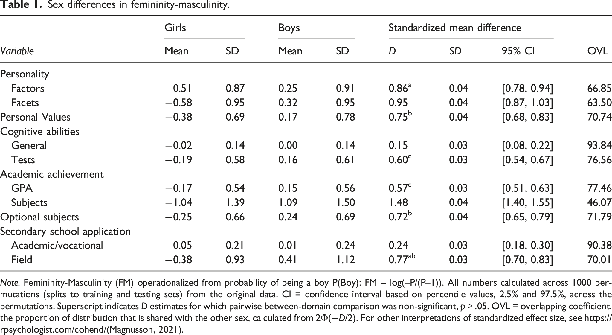
Note. Femininity-Masculinity (FM) operationalized from probability of being a boy P(Boy): FM = log(–P/(P–1)). All numbers calculated across 1000 permutations (splits to training and testing sets) from the original data. CI = confidence interval based on percentile values, 2.5% and 97.5%, across the permutations. Superscript indicates D estimates for which pairwise between-domain comparison was non-significant, p ≥ .05. OVL = overlapping coefficient, the proportion of distribution that is shared with the other sex, calculated from 2Φ(−𝐷/2). For other interpretations of standardized effect size, see https://rpsychologist.com/cohend/(Magnusson, 2021).
Exploratory results
Pairwise comparisons of sex differences between domains with a Q-test (in metafor package; Viechtbauer, 2010) that accounted for the stochastic dependency of the estimates across permutations showed clear heterogeneity. Of all 45 comparisons, 40 showed a statistically significant difference, p < .05. Three groups emerged within which the magnitude of sex differences did not differ: personality factors and applied field of education, Q(1) = 2.44, p = .118, cognitive test profiles and GPA, Q(1) = 0.27, p = .605, and values, optional subjects, and applied field of education, for all three pairwise comparisons p > .335.
As requested by a reviewer, we also, for explorative purposes, calculated Mahalanobis’ Ds for all variable sets. Furthermore, for personality factors and cognitive tests, we calculated Dcorrected which corrects the D-estimates for unreliability in the input variables. We used ωt for personality factors and π(2) for cognitive tests as indicators of reliability. Du, the regularized version of Mahalanobis’ D was also calculated. Because all these calculations were done using the entire dataset (no cross-validation at any stage), we also obtained elastic net D estimates computed from the entire dataset in order to allow for direct comparison and comparable levels of inflation due to overfitting. That is, cross-validation for the elastic net D estimates was run within the training data with k-fold cross-validation, but the data was not split into training and testing sets for subsequent cross-validation.
All estimates from these exploratory analyses are reported in Table S16 in the SOM. There were few substantial differences between methods. Most notably Dcorrected for personality factors was 1.11 whereas elastic net D and Mahalanobis’ D were both 0.89 (the mean estimate with the preregistered cross-validation method was 0.86). Dcorrected for cognitive tests was estimated at 0.76, whereas elastic net D (0.68) and Mahalanobis’ D (0.65) were only slightly lower (the mean estimate with the preregistered cross-validation method was 0.60). Elastic net D estimates for personality facets with the entire data were somewhat higher (D = 1.13) than with the method that separated training and testing data (D = 0.89), which could be due to increased overfitting as the number of variables increases. For variable sets with fewer variables (there were 30 personality facets, whereas for other domains there were at most 16 variables) overfitting was less of a problem, as indicated by smaller differences in elastic net D estimates (see Table S16).
Variance ratio in femininity-masculinity, predictive accuracy of femininity-masculinity, and variance explained by femininity-masculinity.
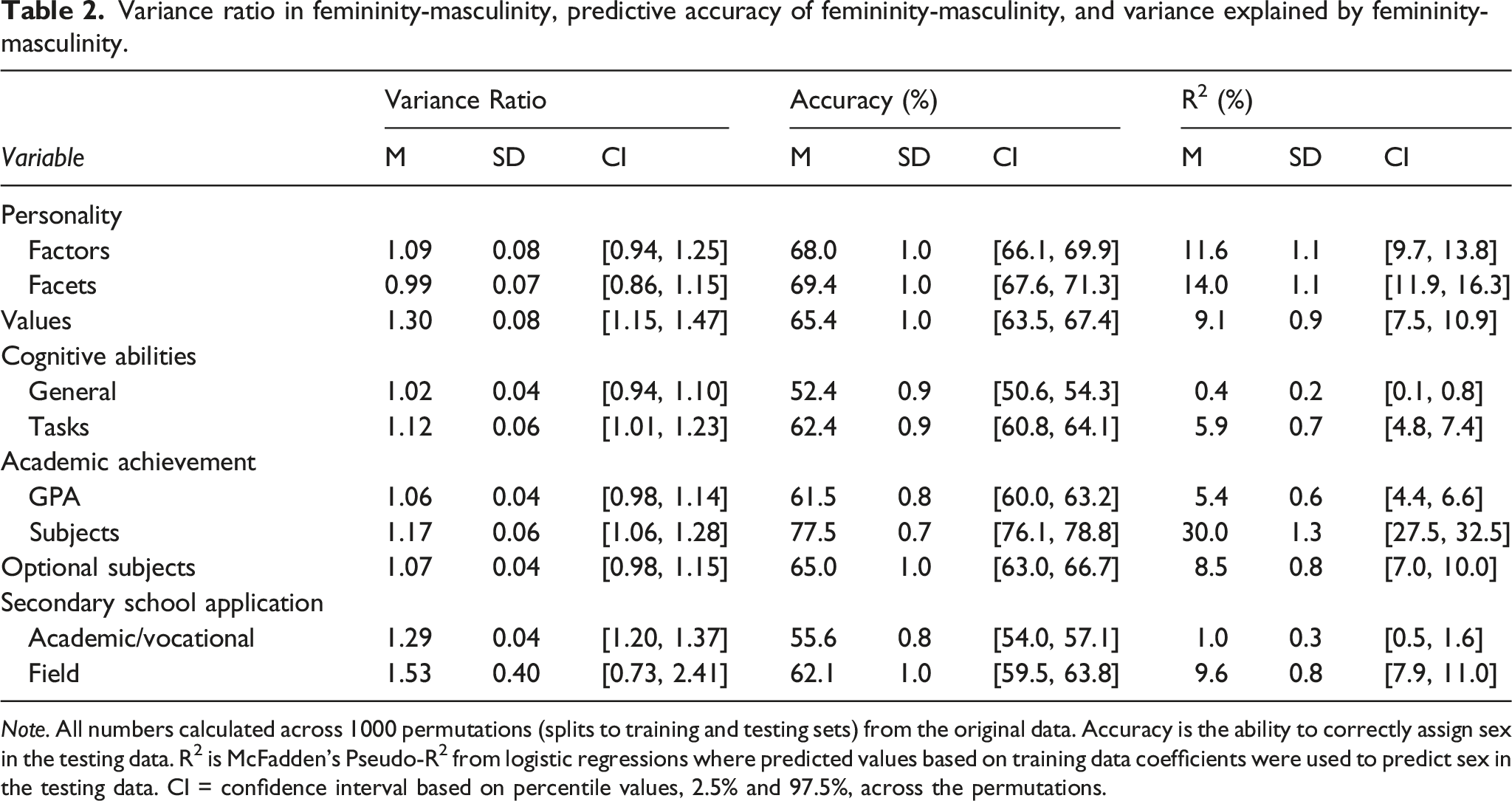
Note. All numbers calculated across 1000 permutations (splits to training and testing sets) from the original data. Accuracy is the ability to correctly assign sex in the testing data. R2 is McFadden’s Pseudo-R2 from logistic regressions where predicted values based on training data coefficients were used to predict sex in the testing data. CI = confidence interval based on percentile values, 2.5% and 97.5%, across the permutations.
Mean gender typicality of girls and boys.
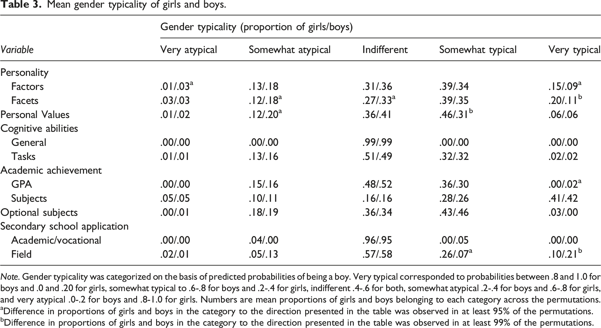
Note. Gender typicality was categorized on the basis of predicted probabilities of being a boy. Very typical corresponded to probabilities between .8 and 1.0 for boys and .0 and .20 for girls, somewhat typical to .6-.8 for boys and .2-.4 for girls, indifferent .4-.6 for both, somewhat atypical .2-.4 for boys and .6-.8 for girls, and very atypical .0-.2 for boys and .8-1.0 for girls. Numbers are mean proportions of girls and boys belonging to each category across the permutations.
aDifference in proportions of girls and boys in the category to the direction presented in the table was observed in at least 95% of the permutations.
bDifference in proportions of girls and boys in the category to the direction presented in the table was observed in at least 99% of the permutations.
In the domain of personality, girls were more often very gender typical than boys were. This was observed for both factors (the mean proportion of very gender typical girls was .15; the corresponding number for boys was .09) and facets (girls = .20, boys = .11). Based on personality factors, boys were more often very gender atypical (girls = .01, boys = .03), and based on personality facets boys were more often somewhat atypical (girls = .12, boys = .18) or indifferent (girls = .27, boys = .33).
In the domain of personal values, girls were more often somewhat gender typical (girls = .46, boys = .31) and boys were more often somewhat gender atypical (girls = .12, boys = .20).
Regarding general cognitive ability and cognitive test profiles, the typicality distributions were similar for girls and boys. For general cognitive ability, 99% of girls and boys were categorized as indifferent, reflecting the small sex difference in this variable.
Reflecting the lower grade-point average of boys, boys (who had very low GPA) were more often categorized as very gender typical than girls (girls = .00, boys = .02). Gender typicality distributions based on the grade profile showed a steady increase towards the very typical category, which was the most common category among both girls and boys (girls = .41, boys = .42). These distributions were not different between girls and boys.
Regarding optional subjects and applying for high school versus vocational institute, there were no sex differences in gender typicality. However, in terms of preferred field of education, boys were more often very gender typical (girls = .10, boys = .21) and girls were more often somewhat gender typical (girls = .26, boys = .07). The majority of the participants was, however, indifferent (girls = .57, boys = .58).
Research question 2: Are narrower measures more informative regarding sex differences and gender?
The predictive utility of each variable set is presented in Table 2. The first index gives the accuracy of correctly predicted sex in the testing data. The second index shows McFadden’s pseudo-R-squared metric obtained from logistic regressions in which FM-scores were used to predict sex. To examine the utility of the narrower measures, we added, within each domain, the narrower measures to logistic regression models that already included the broader measures and looked at whether this improved the models.
Broad personality factors (mean accuracy: 68.0%) were almost as accurate as narrower facets (69.4%) in predicting sex (Table 2). Nevertheless, the preregistered confirmatory tests did show that FM scores based on the facets improved predictive power across permutations (mean log odds = 0.18, 95% CI 0.12–0.24; the mean/median of −2✕log likelihood between the models across permutations was 10.20/10.18, p = .001 for both). Facets also explained more variance than did domains; mean pseudo-R 2 s were 14.0% and 11.6%, respectively.
Confirmatory tests showed that the battery of cognitive tasks was notably more accurate (62.4%) and had more explanatory power (5.9%) than did the general cognitive ability score (mean log odds = 0.23, 95% CI 0.18–0.29; the mean/median of −2✕log likelihood between the models across permutations was 34.72/34.43, p < .001 for both). Both accuracy (52.4%) and predictive power (0.4%) were very low for general cognitive ability.
Regarding academic achievement, confirmatory tests showed that FM-scores based on 16 separate subjects clearly outperformed GPA (mean log odds = 0.16, 95% CI 0.15–0.18; mean/median of −2✕log likelihood between the models across permutations was 141.16/141.33, p < .001 for both). This could be seen both from the former’s higher predictive accuracy (77.5% vs. 61.5%) and the larger proportion of variance explained (30.0% vs. 5.4%).
Comparing a binary measure of preferences for academic level of secondary education (high school vs. vocational institute) with preferences for specific educational field (17 in all) showed a clear advantage for the latter, both in terms of percentage correct (55.6% vs. 62.1%) and variance explained (1.0% vs. 9.6%; mean log odds = 0.16, 95% CI 0.11–0.20; the mean/median of −2✕log likelihood between the models across permutations was 59.04/59.13, p < .001 for both). In sum, narrower measures outperformed broader measures in both psychological (personality and cognitive ability) and academic (academic achievement and educational preferences) domains.
Research question 3: Is femininity-masculinity domain specific or correlated across domains?
Confirmatory results
As alluded to above, after preregistering our research we realized that the zero-order correlations that we planned on presenting would be confounded by sex differences. To clarify, the measure of genderedness employed within the gender diagnosticity approach is computed based on sex differences in a set of attributes and is only meaningful when such differences exist (Lippa & Connelly, 1990). This means that when looking at the associations of genderedness with other variables, these associations will by definition be confounded by sex. Also, correlations between two different measures of genderedness, computed in different domains from a different set of attributes, will invariably be confounded by sex. This means that despite research question 3 being preregistered, we will test it with methods—partial correlations that control for sex and separate analyses within sexes—that were not preregistered. It was necessary to use these methods to avoid confounding by sex (see exploratory results below; Ashton & Lee, 2008; Twenge, 1999).
Although not, as it turned out, pertinent to the present research questions, but for the possible benefit to future meta-analyses in this area, we present, in accordance with the pre-registered analysis plan, the zero-order correlations in Table S17 of the SOM. These zero-order correlations are, of course, higher than the partial and within-sex correlations that we report on, as they include variance that is attributable to the sex of the participant. On a cautionary note, it is important to keep in mind that the sex differences that are controlled for can be of biological, cultural, environmental, or any other conceivable origin—they are descriptive, not explanatory (Del Giudice, in press). That the relationships between FM-score computed from difference domains decrease from zero-order to partial correlations cannot therefore be interpreted as supporting any particular theory regarding the causes of sex- or gender-differences. We also emphasize that research question 3 does not ask whether boys and girls differ (this was covered by research questions 1 and 2). This makes the zero-order correlations, very much confounded by sex differences, rather useless. Instead, we ask whether a boy or a girl who is very boyish or girlish in one domain is likely to be more boyish or girlish also in other domains, and this question can be best answered by looking at partial correlations and within-sex correlations.
Exploratory results
Partial correlations between FM scores.
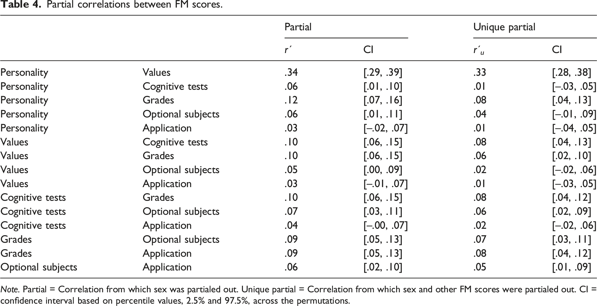
Note. Partial = Correlation from which sex was partialed out. Unique partial = Correlation from which sex and other FM scores were partialed out. CI = confidence interval based on percentile values, 2.5% and 97.5%, across the permutations.
Within-sex FM score correlations.
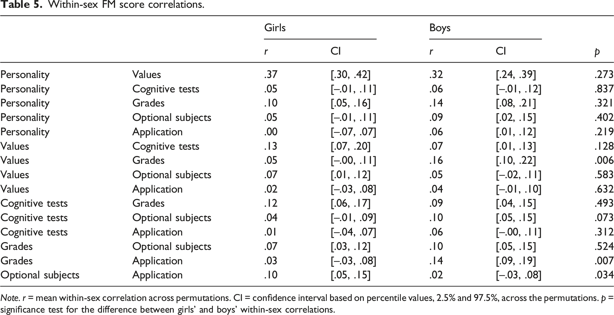
Note. r = mean within-sex correlation across permutations. CI = confidence interval based on percentile values, 2.5% and 97.5%, across the permutations. p = significance test for the difference between girls’ and boys’ within-sex correlations.
As indicated by the partial correlations, femininity-masculinity was correlated across domains. An exception to this was preference for field of education, which showed non-significant correlations with personality, values, and cognitive test profiles, although its associations with grade profiles and optional subjects were significant. The remaining twelve variable pairs were all positively correlated. These associations were, however, not very strong: the average partial correlation was r´ = .09. Clearly, the strongest association was observed between personality FM scores and personal values FM scores, r´ = .34, with none of the other partial correlations stronger than r´ = .12.
The weakness of the observed partial correlations suggests that there may not be a general factor of genderedness, given that a factor should have substantial loadings (e.g., larger than .50) from each of its indicators. A one-factor, maximum likelihood exploratory factor analysis of the correlation matrix supported this interpretation: only personality FM scores and personal values FM scores loaded substantially on this factor (.56 and .59, respectively), whereas cognitive test profiles (.16), grade profiles (.22), optional subjects (.12), and preferred field of education (.07) FM scores loaded only weakly. The factor accounted only 12.6% of the total variation in FM scores (95% CI from 10.9% to 14.5% across separate analyses for each permutation). Results from confirmatory factor analysis, which allow for an interpretation similar to the exploratory factor analysis, can be found in SOM Table S18. Our results thus did not support the existence of a strong genderedness factor.
The absence of a “g-factor” of genderedness led us to interpret the results from a network perspective. This means that we do not assume a unitary common cause in the process that generates the data for various FM scores (as opposed to what latent factor model would assume; Christensen et al., 2020). More generally, the network approach to psychological characteristics understands these networks as complex dynamical systems of interacting variables (van Borkulo et al., 2017). Here, we use this approach to describe the unique and shared links in a network that consists of femininity-masculinity in six different domains. This will tell us whether certain femininity-masculinity scores are conditionally independent (their association can be explained by other FM-scores) or if they are uniquely associated beyond what can be explained by the other measured forms of femininity-masculinity. In addition, the general importance of each FM-score in the network can be estimated from its connectedness with other FM-scores (node strength: Christensen et al., 2020). Finally, global network strength (van Borkulo et al., 2017) can be used to assess the degree of general dependency in the network and for comparison between the networks of boys and girls.
Although global network strength, calculated as the sum of the absolute associations in the entire network was statistically significantly different between partial (1.33) and unique partial (1.04) associations, Q(1) = 16.18, p < .001, this difference was rather modest in size (21.9%). This also showed in the unique partial correlations; only three of the twelve significant partial correlations were rendered non-significant when the other associations were controlled for (between personality and cognitive test profiles, personality and optional subjects, and values and optional subjects). This indicates that several pairs of FM-scores are uniquely associated with each other. The partial and unique partial correlation networks are depicted in Figures 1a and b. Association networks between FM-scores for All Participants (panels a and b), Boys (panels c and d), and Girls (panels e and f). Note. Abbreviations for FM-scores: App = Educational Track Applied for; Cgn = Cognitive Abilities; Grd = Academic Grades; Opt = Optional Subjects Selected; Per = Personality; Val = Values. Associations smaller than .05 were not drawn. Layouts were averaged within each row.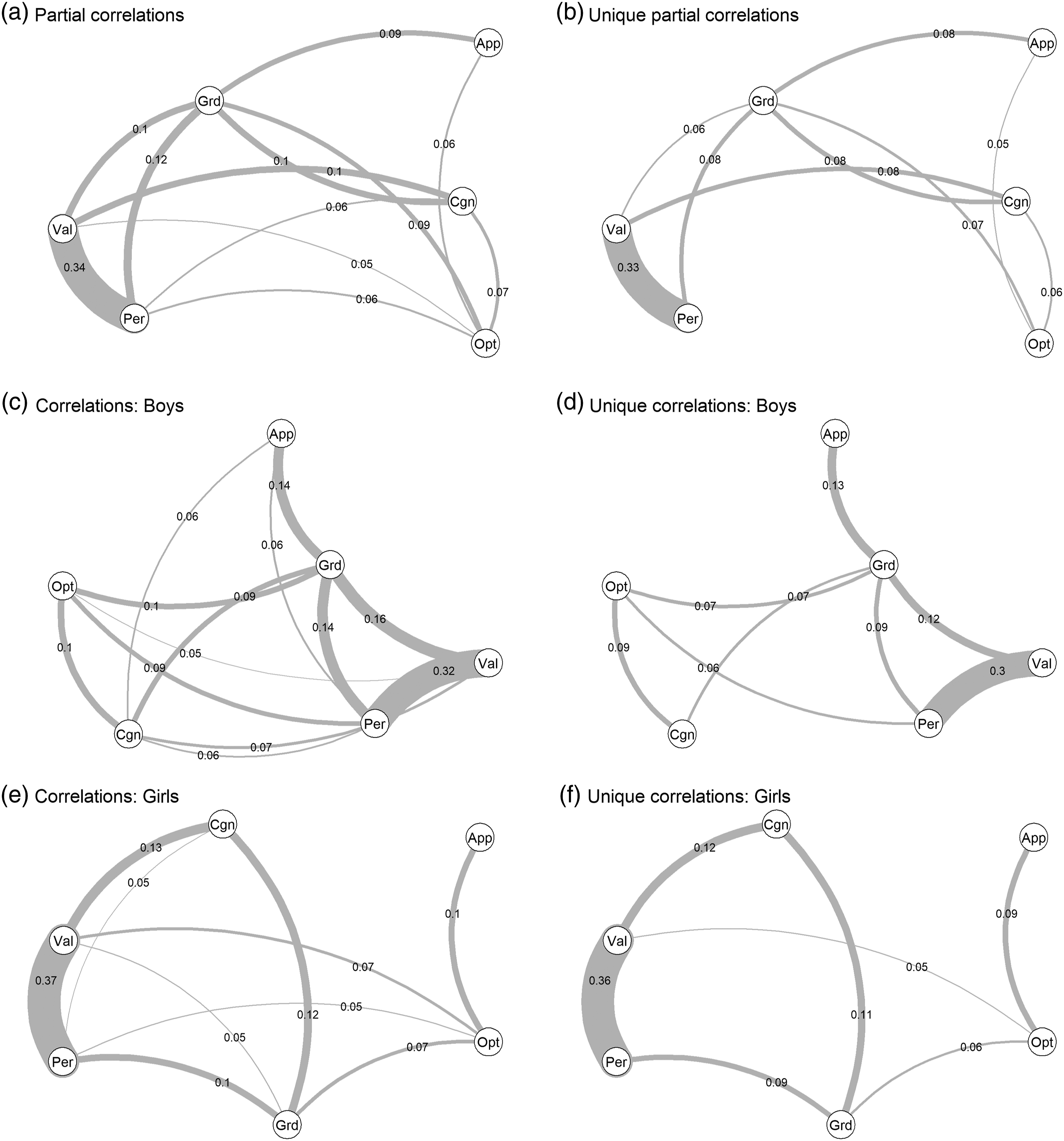
The femininity-masculinity networks of boys and girls are illustrated in Figures 1c–f. The global strengths of the networks (boys = 1.50, 95% CI [1.19, 1.81]; girls = 1.27, 95% CI [1.02, 1.55]) were not significantly different, Q(1) = 1.50, p = .220. The reductions in global network strength when moving from partial to unique partial networks were similar for boys and girls (22.7% and 11.9% drop for boys and girls, respectively, Q(1) = 1.49, p = .222). These analyses indicate that among both boys and girls, femininity-masculinity shows similarly weak generalizability across domains.
Node strengths in partial and within-sex FM-score correlation networks.
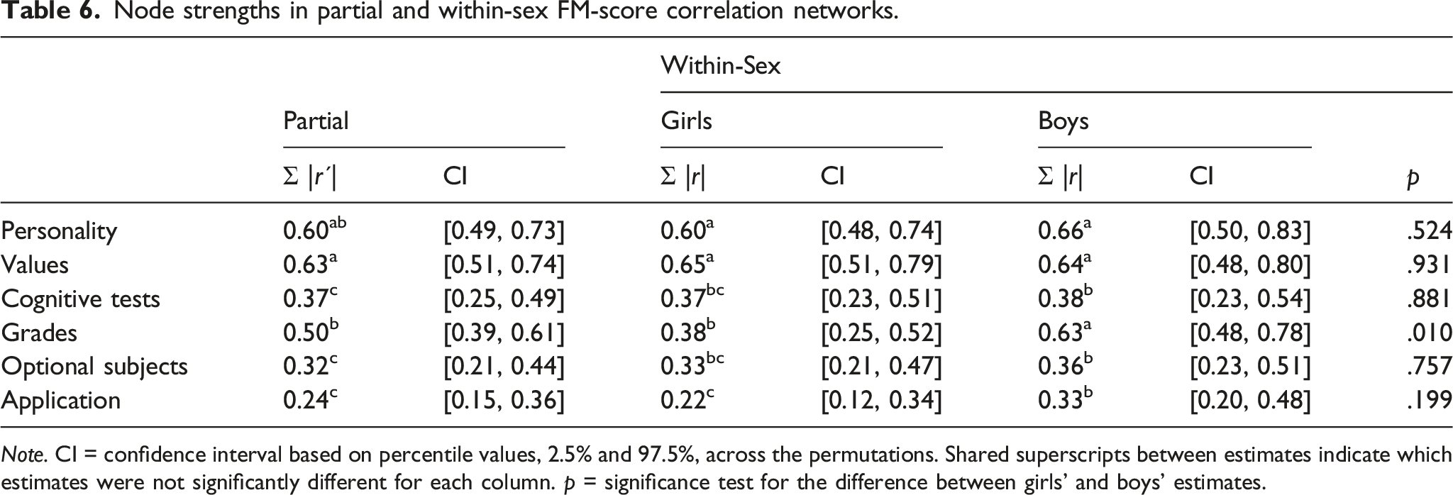
Note. CI = confidence interval based on percentile values, 2.5% and 97.5%, across the permutations. Shared superscripts between estimates indicate which estimates were not significantly different for each column. p = significance test for the difference between girls’ and boys’ estimates.
We finally tested for sex differences in each pair of correlations (Table 5). There were three within-sex correlation estimates that differed between boys and girls. Among boys, the association between the FM-score based on personal values and the FM-score based on grades was stronger than among girls (r = .16 and r = .05, respectively, p = .006). Boys also showed a stronger correlation between FM-scores based on grade profiles and preferred field of education (r = .14 and r = .03, respectively, p = .007). Among girls, FM-scores based on optional subjects and FM-scores based on application were more strongly correlated than among boys (r = .10 and r = .02, p = .034).
In sum, the correlations between FM-scores were weak and did not, despite being generally positive, suggest a general factor of genderedness. More detailed exploratory investigations from a network perspective revealed that femininity-masculinity in personality, personal values, and grade profiles are more central in the femininity-masculinity network than are cognitive test profiles, optional subjects, or preferred field of education. In addition, the grade profile was more central among boys than among girls, which was particularly evident in its stronger associations with femininity-masculinity scores based on personal values and preferred field of education.
Discussion
The present study of Finnish adolescents found that boys and girls differ in personality, values, cognitive aptitude profiles, grade profiles, optional school subjects, and in field of education applied for in secondary education. Very large sex differences were found in grade profiles, indicating that there are several academic subjects in which average girls (boys) perform notably better than average boys (girls) when controlling for performance in other subjects. The grade profiles showed clearly stronger sex differentiation than did personality traits, personal values, or cognitive test profiles, although these also showed medium to large sex differences.
Regarding our second preregistered research question, narrower measures of personality, cognitive ability, academic achievement, and preferences for secondary education outperformed broader measures of these constructs in the prediction of sex, leading to larger sex differences in narrow than in broad measures. Regarding personality, our results are consistent with previous work suggesting that narrow constructs can outperform broad traits in predicting various criterion outcomes (Seeboth & Mõttus, 2018).
Our third preregistered research question asked whether femininity-masculinity in one domain was associated with femininity-masculinity in another domain. To answer this question, we—in contrast to the pre-registered method, which did not control for the confounding role of sex— employed sex-partialed and within-sex associations. Despite our results pointing to the existence of such associations, they were generally very weak, with the one exception that typically girlish (boyish) personality traits tended to go together with typically girlish (boyish) personal values. Because all the associations between domains were in the same direction, it was nevertheless possible to extract a single general factor via factor analysis. Given the extremely low loadings of all but personality and personal values variables on this factor and that it explained only 13% of the total variation in FM scores, we interpret our results as suggesting that there is no “g-factor” of genderedness. We therefore employed the network perspective for further probing of the associations between domains.
On a more exploratory note, we investigated differences in the within-sex variation of FM-scores and found that boys had significantly higher variance in FM-scores based on personal values, cognitive task profiles, grade profiles, and in applying to high school versus vocational institute. In terms of personality and values, there were more gender typical girls than there were boys. However, in terms of preferred field of education, there were more very gender typical boys.
The discussion focuses on the comparison of sex differences across domains and on what implications these findings have for future developmental studies. Academic achievement profiles are highlighted because they showed the largest sex differences and network analysis indicated their central role in within-sex femininity-masculinity associations.
Overall sex differences in adolescence
Although boys and girls differed in all domains, the size of the gender gap varied widely between domains. The gender gap for personality was large (D = 0.95), and only slightly smaller than the gender gap reported on in a sample of Finnish adults (based on 30 personality facets, Mac Giolla & Kajonius, 2019, reported a gender gap of D = 1.16). This suggests that overall sex difference in personality have almost plateaued in adolescence. Future studies should investigate whether overall sex differences in personality increase from childhood to adolescence, and if so, whether this is because initially small differences in given traits increase or because altogether new traits start showing sex differences.
Studies that have used multi-group covariance and mean structure analysis (Del Giudice et al., 2012; Kaiser, 2019; Kaiser et al., 2019) have reported notably larger sex differences than those we report on (often D > 2.0). We could not employ latent variable modeling at the facet level because we did not have multi-item scales at that level. However, some theoretical consideration also advice against the use of latent variable modeling. First, it has recently been established that there is meaningful variation also at the lowest level of the personality structure; nuances or single personality scale items show unique longitudinal stability, heritability, interrater-agreement, and predictive utility (Mõttus et al., 2017, 2019). By focusing only on the common variance that is shared by a set of items, or relying on a parceling method that enforces the communality of input variables in latent variable models (Booth & Irwing, 2011; Del Giudice et al., 2012), a large proportion of meaningful personality variation could be neglected. Also, the present results testify to the importance of item level variation—facet-trained femininity-masculinity scores outperformed factor-trained femininity-masculinity scores in the prediction of sex, thus also showing larger sex differences than factors (see Mac Giolla & Kajonius, 2019, for similar result). Second, latent variable modeling that aims to minimize measurement error makes strong assumptions regarding the data generation process. This approach could thus lead to severe bias and inconsistency in estimation, even in comparison to composite scales, which are also systematically biased (Rhemtulla et al., 2020). On the other hand, factor scores—sometimes computed in this type of research (Kaiser, 2019; Kaiser et al., 2019) —would have introduced other biases into our multivariate sex difference estimates (see Devlieger et al., 2016). In sum, although our predictive approach, because it does not account for measurement error, may give a somewhat attenuated estimate of sex differences, the bias is very likely to be smaller and certainly more consistent than the various types of bias that latent variable modeling procedures would have introduced—the former involve multiple decisions in the analytical pipeline (the use of items or parcels as inputs, the item parceling approach, examining model fit and change in fit following invariance constraints, model estimates or factor scores, factor scoring method, etc.) and theoretically strong assumptions regarding the data generation process.
For the other domains besides personality and academic achievement, the present study was the first to describe the overall sex differences. Medium to large sex differences—but smaller than sex differences in personality—were found for values (D = 0.75), optionally selected school subjects (D = 0.72), preferred field of secondary education (D = 0.77), and cognitive test profiles (D = 0.60). Sex differences in univariate indices were also observed: large in GPA (d = 0.57, girls score higher), small in academic/vocational educational track (d = 0.24, girls more often applied to academic track), and very small in general cognitive ability (d = 0.15, girls scored higher).
Regarding sex differences in personal values, previous studies have reported very small sex difference in single values (median d = .15 across values; Schwartz & Rubel, 2005). Our results suggest that the overall gap in personal values is, by contrast, large. As in the domain of personality, the overall gap that we report on can be argued to be a better measure of sex differences than average univariate distances (Del Giudice, 2009; in press). This may be even more so in the case of personal values, as the ten basic values are not independent of each other but the total pattern of conflict and compatibility among the values forms a circular structure in which adjacent values reflect compatible motivations and opposing values reflect conflicting motivations (Schwartz, 1992). Schwartz and Rubel (2005) showed that cross-culturally, sex differences were most pronounced for power (men higher) and for benevolence (girls higher) values, and are results corroborate this finding in an adolescent sample. These two values were the largest contributors to the overall gender gap, followed by significant but smaller contributions from universalism (girls higher) and tradition (boys higher). The six remaining values did not reliably contribute to the overall sex difference in values. Future studies on the gender gap in values should employ the here presented methodology to adult populations, especially within a cross-cultural framework. Schwartz and Rubel (2005) reported that the largest sex differences in benevolence and power values were found in more egalitarian countries, and research on personality traits suggests that overall sex differences are larger in more egalitarian countries (Mac Giolla & Kajonius, 2019). Together these results suggest that the overall gender gap in values could also be largest in more egalitarian countries, something that could be investigated with the many large-scale cross-cultural surveys that include values measures.
Although there were no meaningful sex differences in general cognitive ability, the performance profiles on cognitive tests did show a medium-to-large gender gap that indicated more sex differentiation than has usually been reported for single cognitive abilities (Halpern, 2011; Hedges & Nowell, 1995; Miller & Halpern, 2014; but see Lauer et al., 2019 and Lynn & Irwing, 2002 for moderate differences in some mental rotation task variants and general knowledge, respectively). This implies that the common practice of summarizing across tasks tends to mask differences in how the sexes perform across a set of tasks (Johnson & Bouchard, 2007). However, this difference should not be overstated. The magnitude of the sex difference in cognitive test profiles was similar to that of the sex difference in general academic achievement, GPA. Stated differently, the cognitive test score profile based on nine different cognitive tests gave as accurate a prediction of which sex any individual was as did the single GPA score (the accuracies were 62.44% and 61.66%, respectively). Such predictions and comparisons are, of course, in some sense senseless, but do provide an intuitive metric about how (un)informative cognitive tests can be regarding sex.
The by far largest gender gap was found for grade profiles, which showed a very large sex difference (D = 1.48). Another recent cross-cultural study on a more limited set of achievement variables also indicated large overall sex differences (Ds ranged between 0.75 and 1.26) (Stoet & Geary, 2020). The expectancy-value model (Wigfield & Eccles, 2000) has gained some traction in explaining sex differences in grades. For instance, boys’ lower reading grades have, in the absence of actual differences in reading skills, been explained by lower parental expectations and by lower self-assessed importance of reading (Heyder et al., 2017). Sex differences in parental expectations and self-assessed importance could vary from subject to subject (e.g., boys could be expected to perform better in physics), which could help explain the large overall gender gap in grade profiles. Importantly, the difference in grade profiles was much larger than the difference in cognitive test profiles, suggesting that something else than sex differences in cognitive ability is needed to explain the differences in grade profiles. Also speaking against differences in actual cognitive ability as explanations for the gender gap in grades, subjects that could be expected to rely heavily on the same set of cognitive abilities showed opposite direction associations with sex. For instance, both native language and history could be expected to rely heavily on reading skills, but high grades on the former were associated with being a girl and high grades on the latter with being a boy. Finally, the cognitive ability test was administered in a low-stakes research context, suggesting both that motivation will vary and that this will influence test scores (Duckworth et al., 2011; Kupiainen et al., 2014). This means that performance on a particular cognitive ability test might very much depend on the self-assessed importance of the skill being tested. In fact, in a different sample of Finnish 16-year-olds that completed a very similar battery of cognitive ability tests, controlling for self-reported effort and for amount of time spent responding rendered sex-differences insignificant (Vainikainen & Hautamäki, 2018). Finally, sex differences in interests (Su et al., 2009) could independently add to investment in subject specific performance. This all adds up to suggesting that something else than cognitive ability profiles, be it parental expectations, self-assessed importance, and/or interest, is needed to explain the differences in grade profiles. Future research should investigate parental expectations and self-assessed importance of and interest in the academic subjects in order to evaluate whether these constructs could help explain the observed overall gender gap in grades.
Academic grade profiles allowed for rather accurate statistical predictions of sex (accuracy 77.53%). Interestingly, this is very close to the classification of sex obtained with PISA scores and academic attitudes in 2009 and 2012 in Finland (Stoet & Geary, 2020). This could have practical implications when grades and grade profiles are being assessed in application and selection processes. For instance, when assessing university applicants’ academic grades as part of an ostensibly sex-blind selection procedure, the assessor might rather accurately guess the sex of the applicants. Future studies could investigate to what extent people can predict sex from grade profiles, and whether this is a skill that people improve in with experience.
We report on sex difference at the very end of adolescents’ primary education. An interesting question for future research is whether sex differences increase over the years. Given that the differences in grade profiles were so much larger than any other sex differences, these are likely to have, in part, developed during the school years, perhaps through at least some of the various processes outlined by the expectancy-value model (Wigfield & Eccles, 2000). The very large sex differences also showed in the gender typicality examinations, with around 70% of boys and girls classified as at least somewhat gender typical in terms of their grade profiles. Of course, a substantial proportion was not gender typical, and sex differences in grade profiles should not be interpreted as being even close to taxonic (Carothers & Reis, 2013).
In sum, sex difference was found across domains, and the magnitude of these overall differences was non-negligible, except for general cognitive ability. This strongly speaks against the idea that most psychological sex differences are small and meaningless (Hyde, 2014).
The gender distributions of boys and girls do not mirror each other
Not only were mean scores different, but also variance in femininity-masculinity was different across sexes. Regarding personality traits and personal values, girls tended to be more gender typical than boys, with more girls classified as gender typical and more boys classified as somewhat gender atypical. Consistent with this, boys showed more within-sex variation in personal values. Moreover, boys showed more variation also in cognitive abilities and in academic grades, indicating that in these three domains, two randomly selected boys are more likely to be further apart from each other in terms of femininity-masculinity than would be two randomly selected girls.
The above-described type of differences in intra-sex variability has been on a common theme in the literature on cognitive abilities, with both men (Hedges & Nowell, 1995) and boys (Johnson et al., 2008; Strand et al., 2006) showing more intra-sex variability. Some research suggests that similar differences may exist in the realm of adult personality traits, with men showing higher intra-sex variability in informant (but not self-) reports of personality (Borkenau et al., 2013). By contrast, one of our more novel results is the larger intra-sex variance of boys in terms of personal values. In fact, the largest variance ratio that we found was for values (VR = 1.30). For comparison, the variance ratio for human height is 1.11 (more variation among men: Lippa, 2009). This difference in intra-sex variance in values is also reflected in that girls were more often than boys classified as somewhat gender typical (46% vs. 31%) and less often as somewhat gender atypical (12% vs. 20%).
Within-sex heterogeneity in personal values may reflect sex differences in the looseness-rigidity of gender roles (Wood & Eagly, 2015). Most girls had somewhat or very girlish values, whereas boys’ values were more evenly spread across the boyish-girlish continuum. Given that gender-role expectations influence the development of values, these expectations may be more stringent for girls. For instance, girls may be expected to consider and value the well-being of other people (higher Benevolence, Universalism, lower Power), whereas such expectations may be lower for boys. In societies in which the sexes should, on paper, be equal, this type of abstract and difficult to measure gender role expectations can be an important source of continuing inequality.
Regarding preferences for field of secondary education, the above pattern is reversed. Boys were more gender typical: 21% of boys applied for a field classified as very gender typical, as opposed to 10% of girls. In none of the other domains except for grade profiles was there such a high proportion of the participant pool being classified as very typical. The simplest explanation is probably that a large proportion of boys prefer certain fields that are preferred primarily by other boys (another possible explanation, some form of “strategic” thinking in which boys consider what is realistic given their lower grades is less likely—participants could apply to as many as five different institutions, suggesting that their first choices, which we used, could be indicative of actual preferences).
The above pattern, in which boys are in some sense freer in terms of personal values but more constrained in terms of educational preferences, is intriguing. Explanations referring to possibly stronger biological or genetic hard-wiring of values, as compared to educational preferences, would have one expect at least as strong between-sex differences in within-sex variance in personality traits. Personality, in which boys did not show greater intra-sex variability than did girls, overlaps with values but has been argued to be more hard-wired in terms of biological basis, with values being formed by both personality traits and by external influences, such as culture and life events (McCrae & Costa, 2008). This implies that external influences allow boys more agency or freedom of choice in terms of what they value in life. However, when push comes to shove; that is, when sixteen-year-olds decide where to apply for secondary education, a decision they may perceive as being the most consequential decision of their life so far, boys end up behaving like other boys. Making this pattern even more intriguing, is that values, empirically associated with perceptions, attitudes, goals, and behaviors (Maio, 2010; Roccas & Sagiv, 2010), would be expected to also be associated with important life choices. However, other than a study that showed that police officer recruits differ from the general population in terms of their values (Bardi et al., 2014), there is very little empirical evidence that would support a link between personal values and career choices.
The literature on gendered career choices and the distribution of men and women in the labor force has very much focused on women’s lower interest in male-dominated occupations especially those in science, technology, engineering, and math (e.g., for a review on the gender gap in STEM occupations, see Wang & Degol, 2017). Much less attention has been given to factors that contribute to men’s disinterest and underrepresentation in female dominated occupations (Shen-Miller & Smiler, 2015). Our results suggest that it is boys or men who, despite showing more intra-sex variation in their values, may be making the more gender stereotypical choice. This implies that other factors than personal values, such as culturally dictated occupational gender stereotypes (Forsman & Barth, 2017) or the male-breadwinner norm (although this is in decline in Scandinavia, it is not a thing of the past, Edlund & Öun, 2016; Leira, 2006) may constraint men’s choices. A complimentary line of explanation could be that it is not so much the fields of education that matter, but boys’ higher gender homophily: boys may, in part, make the career choices they make in order to be able to study and work together with other boys (men and boys have more gender homophilous networks and friendships than do women, e.g., Benenson et al., 2012; McPherson et al., 2001). This should be an interesting topic for future investigations.
No support for a g-factor of genderedness
Our third research question concerned the generality of femininity-masculinity across psychological and educational domains. Although the associations between femininity-masculinity in one domain and femininity-masculinity in another domain were all positive, they were far too weak to suggest the existence of a unitary common source of variation shared between different femininity-masculinity scores. We therefore wish to emphasize that in the case of genderedness, despite reporting on a positive manifold, we do not believe that the present data in any way suggests the existence of a general factor of genderedness. There were, nevertheless, positive associations between the femininity-masculinity indices based on different domains, and alternative explanations of this positive manifold are needed.
We examined the associations between femininity-masculinity in different domains in terms of the network approach, which provides indices summarizing the role of single associations in the global network of associations without presupposing the existence of a general factor. With one exception, the femininity-masculinity scores based on different domains were weakly albeit positively correlated. The by far strongest association was found between self-reported personality traits and personal values. Although the strength of this association might partially reflect shared method variance, it is also likely to reflect substance. Previous research has shown that self-direction values are strongly correlated with trait openness to experience and that benevolence values are strongly correlated with trait agreeableness (Parks-Leduc et al., 2015). Because these constructs overlap, also genderedness scores based on these constructs would be expected to overlap. Informant reports of personality would shed some light on the size of the overlap in the absence of variance attributable to the source of the ratings. Because femininity-masculinity in personality shows trait-like properties in terms of temporal stability and heritability (Loehlin et al., 2005), it could be expected to show trait-like properties also in terms of self-other agreement. As this tends to be rather high, variance attributable to the source of the ratings may not have distorted our results that much.
Personality and values were also the more central nodes in the femininity-masculinity networks. Perhaps more interestingly, in terms of not owing its centrality to construct overlap or method variance, grade profile femininity-masculinity was also central, especially in the femininity-masculinity network of boys. The correlational evidence that we have does not allow for inferences regrading causality but, its connectedness with other forms of femininity-masculinity suggests that academic grade profiles would be a good place to start the search for the more important determinants and consequences of gender typicality. Grade profiles are not only relevant for understanding sex differences, but also for understanding within-sex femininity-masculinity associations.
Although the bivariate associations between boyishness (girlishness) in one domain with boyishness (girlishness) in another domain are weak, they are consistently found across domains, suggesting some degree of generalizability. At least some of the unique associations could allow for substantive interpretations. For example, boyish (girlish) grade profiles and boyish educational preferences could have a mutual cause and/or they could reciprocally reinforce each other. Also, differences between boys’ and girls’ networks could have meaningful interpretations. Femininity-masculinity in grades and values were more strongly associated among boys than among girls. This could, again, speak to sex differences in the looseness-rigidity of gender roles (Wood & Eagly, 2015) and perhaps also to different expectations regarding school performance; shrugging our collective shoulders in resignation and saying “boys will be boys” when it comes to performance in some subjects, such as reading, may set the bar much too low (Kimmel, 2006). On the most general level, the stronger association between grades and values in boys’ as compared to girls’ networks could be explained by the greater freedom of boys; both to endorse whichever values they wish to endorse and to perform less consistently across school subjects.
The unique associations (associations in which variance in all the other domains was controlled for) between femininity-masculinity scores were not much weaker than the associations in which only sex was controlled for. This again speaks against a common source of variation in femininity-masculinity across domains. That different FM-scores are not redundant suggests that a general cross-domain form of femininity-masculinity is best understood as a complex dynamical system of weakly interacting domain-specific indices of femininity-masculinity (van Borkulo et al., 2017). Therefore, rather than aiming for parsimony in understanding femininity-masculinity, future research should first focus on comprehensively covering various forms of femininity-masculinity. The network approach to gender diagnosticity would then allow for examining the unique components and communities that such a system would be comprised of (Christensen et al., 2020). Despite the absence of a general factor of genderedness, there could be communities comprised of a limited set of certain forms of femininity-masculinity. For example, separately calculating FM-scores for each of the five personality factors from self- and informant-reports would allow for the examining the possibility of finding a community that could be labeled “femininity-masculinity in personality” and/or whether some scores would also be uniquely associated with femininity-masculinity in non-personality domains.
Limitations and future directions
Although the administered battery of cognitive tests did include nine different measures, it may have left out specific areas of cognitive ability. For example, some tests for which some of the larger sex differences have been documented were not included. A recent meta-analysis suggests that the sex difference at 16 could be roughly between d = 0.40 and d = 0.60 for mental rotation (Lauer et al., 2019), and a sex difference of similar magnitude was reported for general knowledge in a study of undergraduates in the UK (Lynn & Irwing, 2002). However, because mental rotation and general knowledge presumably show at least moderate correlations with some, if not all, of the cognitive tests that we did administer, these sex differences cannot in any straightforward way be added to the multivariate estimate we obtained. Nevertheless, sex differences in any domain should ideally be studied using the most comprehensive and broad set of variables, with the emphasis on variables that have been previously known to show sex differences. This applies not only to cognitive tests, but also to other domains, such as personality and values, of which the latter was measured with only ten items.
Another limitation is that NCS personality items used in the present study were single-item measure of personality facets. Not all facets, let alone narrower nuances, are included in this type of measure that has been designed top-down with the intention to measure broad domains such as the Big Five. Personality taxonomies that take a bottom-up approach (e.g., Condon et al., 2020) would include a richer set of personality nuances and facets, which could describe larger multivariate sex differences and allow for better predictions of sex.
Relatedly, irrespective of whether a prediction-focused strategy or a more explanatory approach is used, it is important that the measurement scales used in the multivariate set are reliable. Even when classical test theory reliability indices do not apply, it is important in other ways to show that the input variables are consistent (Christensen et al., 2020; McCrae, 2015). In the present study, such indices were not available for all variables (value items and personality facets) and reliabilities on some scales were quite low (openness to experience, reading comprehension, multiple-choice, and verbal proportional reasoning) which may have led to some inaccuracies in estimation. Comparisons of disattenuated Mahalanobis’ D estimates with other estimates nevertheless indicated that the degree of possible underestimation due to unreliability was small (see SOM Table S16).
Regarding underlying causes, it is important to note that our results are merely descriptive, not explanatory, in a similar way that sex differences are (Del Giudice, in press). They do not speak to questions of why the sexes differ in genderedness or why certain femininity-masculinity scores are correlated and others are not. Our results fit social role theory just as well as evolutionary views, as both social roles and biological factors can have contributed to sex differences and to the genderedness of particular individuals.
Given that there is no general factor of genderedness, an interesting question for future research could be which domains are most relevant for determining whether someone is perceived as girlish or boyish. That is, what constitutes girlishness or boyishness in the eyes of the perceiver? It could be one of the domains that we assessed, or it could be something different, such as playing style or appearance. Investigating associations between girlishness and boyishness in different life domains, and determining which domains are central in determining how the person is perceived, should be interesting questions for future research.
Of course, perceptions of girlishness and boyishness are likely to vary across cultures, cohorts, and perceivers. Furthermore, and even more pertinent to the present research, sex differences and gender roles also vary across cultures. In Finland, sex differences in many of the characteristics that we investigated are particularly pronounced as compared to other countries. For instance, sex differences in personality traits (Mac Giolla & Kajonius, 2019), as well as in PISA performance and career choices (Stoet & Geary, 2018), are larger in Finland than in most other cultures. To what extent our findings regarding sex difference, gender typicality, and the lack of a general factor of genderedness replicate in other cultures should be interesting questions for future research.
Conclusions
The present research updates the gender diagnosticity approach by employing penalized logistic regression to estimate multivariate sex differences based on both binary and continuous variables. The method allows for the robust and seamless integration of sex difference and gender typicality examinations, as well as various types of between sex comparisons regarding the variability and connectedness of different indices of femininity-masculinity. The methods introduced here can be applied in future studies that seek to investigate the development of sex differences and genderedness in multivariate frameworks.
Besides the methodological advancements, the present research, being the first to investigate the associations between gender typicality in different domains, also has several substantive contributions. First off, we estimate the magnitude of adolescents’ sex differences in various psychological characteristics and in educational attainment and aspirations. Our results show that the magnitude of these differences varies a lot from domain to domain, and it will be highly interesting to compare the size of the differences that we report on with differences found in other age groups or in other cultures. Second, our results suggest that gender typicality, a theme that to date has not received the same research attention as sex differences, could offer important insights into the role of gender in shaping people’s lives. For instance, speaking to the normative pressures of gender roles, girls reported more gender typical personal values, but boys were more often gender typical in terms of educational choices. Third, narrower measures, especially grade profiles, were generally very good at predicting sex, suggesting a potential risk for sex-bias even in sex-blind evaluation contexts. Finally, our results suggest that there is no such thing a typical boy or a girl: boyishness in one domain, such as personality, is only very weakly related to boyishness in other domains, such as cognitive profile or academic grades. When discussing boyishness or girlishness, a specifying clause giving more information should always be added.
Supplemental Material
Supplemental Material - Is there a g-factor of genderedness? Using a continuous measure of genderedness to assess sex differences in personality, values, cognitive ability, school grades, and educational track
Supplemental Material for Is there a g-factor of genderedness? Using a continuous measure of genderedness to assess sex differences in personality, values, cognitive ability, school grades, and educational track by Ville-Juhani Ilmarinen, Mari-Pauliina Vainikainen, and Jan-Erik Lönnqvist in European Journal of Personality
Footnotes
Declaration of conflicting interests
The author(s) declared no potential conflicts of interest with respect to the research, authorship, and/or publication of this article.
Funding
The author(s) disclosed receipt of the following financial support for the research, authorship, and/or publication of this article: This research was supported by the Academy of Finland research grant 338891 to V.-J. I. and by the Academy of Finland research grant 309537 to J.-E. L.
Data accessibility statement
In agreement with the Education Department of the city where the study was conducted, the data are stored on a private university network to which researchers can gain access only by application and no part of the data are allowed to be downloaded from that network to another location. Doing so would be a breach of contract. Thus, the data are not available. Materials and analysis scripts with related results output are available at ![]() . A preregistration for the study can be found at https://osf.io/6ksz9.
. A preregistration for the study can be found at https://osf.io/6ksz9.
Supplemental Material
Supplemental material for this article is available online.
References
Supplementary Material
Please find the following supplemental material available below.
For Open Access articles published under a Creative Commons License, all supplemental material carries the same license as the article it is associated with.
For non-Open Access articles published, all supplemental material carries a non-exclusive license, and permission requests for re-use of supplemental material or any part of supplemental material shall be sent directly to the copyright owner as specified in the copyright notice associated with the article.