
Abstract
There are massive literatures on initial attraction and established relationships. But few studies capture early relationship development: the interstitial period in which people experience rising and falling romantic interest for partners who could—but often do not—become sexual or dating partners. In this study, 208 single participants reported on 1,065 potential romantic partners across 7,179 data points over 7 months. In stage 1, we used random forests (a type of machine learning) to estimate how well different classes of variables (e.g., individual differences vs. target-specific constructs) predicted participants’ romantic interest in these potential partners. We also tested (and found only modest support for) the perceiver × target moderation account of compatibility: the meta-theoretical perspective that some types of perceivers experience greater romantic interest for some types of targets. In stage 2, we used multilevel modeling to depict predictors retained by the random-forests models; robust (positive) main effects emerged for many variables, including sociosexuality, sex drive, perceptions of the partner’s positive attributes (e.g., attractive and exciting), attachment features (e.g., proximity seeking), and perceived interest. Finally, we found no support for ideal partner preference-matching effects on romantic interest. The discussion highlights the need for new models to explain the origin of romantic compatibility.
Our collective understanding of the psychological process by which people evaluate romantic partners has traditionally derived from two research designs. First, initial attraction designs examine how people evaluate a potential romantic partner depicted in a photograph or a vignette (e.g., Brandner et al., 2020; Hitsch et al., 2010; Lee et al., 2008; Townsend & Levy, 1990) or in a face-to-face interaction in the laboratory or on a speed-date (e.g., Back et al., 2011; Eastwick et al., 2011; Luo & Zhang, 2009; Olderbak et al., 2017). In virtually all cases, however, studies of initial attraction conclude after the participant reports a single evaluative judgment; there is no information about how these relationships might have changed and developed over time. Second, close relationships designs often examine the way people evaluate their dating or married partners longitudinally (for reviews, see Berscheid, 1999; Finkel et al., 2017; Reis, 2007). But the near-universal inclusion criterion for a close relationships study is that participants need to indicate that they are involved in a committed, “official” relationship. In other words, people’s experiences are only included in the close relationships literature when they can report on a specific partner whom they are (at least) dating; relationships that never make it that far are empirical ghosts.
In conjunction, these two methodological limitations mean that the published literature largely omits whatever takes place after an initial interaction and before relationship formation (Campbell & Stanton, 2014; Eastwick et al., 2019b). Critically, this early relationship development period is likely to be more than a few days: Typically, people report retrospectively that they knew their partners as friends or acquaintances—often getting to know them over a period of weeks or months—before the relationship became romantic or sexual (Brinberg et al., 2021; Eastwick et al., 2018; Kaestle & Halpern, 2005; Stinson et al., 2022; Walsh et al., 2014). Presumably, it is during this understudied period that single individuals’ waxing and waning romantic interest functions as a critical factor that determines which relationships have a chance to mature and which will remain in a perpetual state of “what if?”
The current study tracked fluctuations in romantic interest of more than 200 single participants over a period of 7 months as they considered over 1,000 different potential romantic partners. No prior work had examined this portion of the relationship arc in such detail. Therefore, we began our investigation by examining the explanatory power of two broad classes of constructs: individual differences (e.g., relationship-relevant traits and motivations), and target-specific constructs (e.g., participants’ judgments about a particular potential partner). We also examined the meta-theoretical perspective that certain perceivers are especially compatible with certain targets (e.g., perceiver × target moderation approaches). To perform these tests, we used random forests (a form of machine learning) to extract estimates of how strongly different batches of variables predict initial report, peak, final report, and change in romantic interest (see “analysis plan stage 1” below).
Random forests offer a novel way to identify which predictors are likely to be especially robust, but by themselves, such methods do not yield a user-friendly visualization of growth curves and effect sizes. Thus, in an effort to bridge the new and classic approaches, we further examined each predictor that emerged in (at least) one of the random forests models using multi-level models (see “analysis plan stage 2” below). In this stage, we also performed a focused test of a perceiver × target perspective by analyzing whether participants were especially interested in potential partners whose attributes matched their a priori ideal partner preferences—a hypothesis that had never been examined in this context. We ground our investigation in classic and novel theories that have discussed the processes by which people gauge whether or not they are romantically compatible with a specific romantic partner.
Early relationship development
Theoretical conceptualizations and challenges
Relationship science is home to a variety of theories that depict the process by which people develop and maintain romantic relationships (for reviews, see Bradbury & Karney, 2019; Finkel et al., 2017). Even though these many theories were primarily developed using data on established couples, the theories themselves typically do not posit a switch that turns components of the theory “off” prior to the official formation of the relationship and “on” afterward. For example, the gradual process of building intimacy via self-disclosure (Reis & Shaver, 1988) likely begins prior to the formation of a dating relationship, the vulnerabilities associated with low self-esteem or high attachment anxiety (Murray et al., 2006) should presumably cause someone to be wary of both initiating a new relationship and deepening an existing relationship, and the “investment” construct in the investment model of commitment (Rusbult et al., 2012) is a continuous variable that can range from very low (e.g., a plan to meet up for coffee) to very high (e.g., raising children and owning a home together). It is even common for scholars to derive new insights about people’s first impressions of strangers by drawing from close relationships theories on attachment (McClure & Lydon, 2014), social exchange (Sprecher et al., 2013), capitalization, (Reis et al., 2010), and self-expansion (Vacharkulksemsuk & Fredrickson, 2012), just to name a few. In this light, it is reasonable to conceptualize the decision to form an official relationship as one step in the multistep process of creating a long-term, stable, happy partnership (Baxter & Bullis, 1986; Lloyd & Cate, 1985), and so major relationship theories could presumably retain some applicability to the portions of the relationship trajectory that precede this event (see also Sprecher et al., 2008).
Of course, some perspectives do contain a specific focus on the way that relationships might develop (or fail to develop) during this stretch of time. Knapp’s (1978; Knapp et al., 2013) classic relational development model proposes that prospective romantic partners move through stages of escalating self-disclosure and interdependence when forming a relationship, and two of these stages—experimenting with self-disclosure and intensifying through expressions of affection—take place after an initial interaction but before a couple-level identity has coalesced. A more recent example of this approach is the ReCAST model (Eastwick et al., 2018, 2019b), which proposes that prospective partners attempt to assess compatibility during early relationship development, and it takes time for people to ascertain whether a given relationship has short-term (i.e., only sexual) potential, long-term (i.e., sexual and attachment) potential, or no potential at all. Qualitative work on the hookup culture of college campuses suggests that students often feel compelled to suppress intimacy in casual sexual relationships, which consequentially limits their opportunity to form relationships that are both sexual and attached (Wade, 2017). These (early-relationship-specific) perspectives collectively suggest that early relationship development is a volatile period of discovery and uncertainty (Clark et al., 2019; Tennov, 1979) such that people’s feelings about a potential partner may be in flux as new information emerges and new experiences occur.
Nevertheless, very little empirical evidence exists regarding the trajectory of romantic interest during the time period that precedes actual relationship formation, and even less evidence exists on such trajectories in relationships that never actually become dating relationships. A number of studies (primarily in the sexuality and adolescent health literatures) examine college hookups, “friends-with-benefits,” and related phenomena (e.g., Calzo, 2013; Fielder et al., 2013; Garcia et al., 2012; Harden, 2014; Jonason et al., 2011; Lehmiller et al., 2014; Owen & Fincham, 2012; Wesche et al., 2018). But these studies do not typically track people’s relationships with the same hookup partners over multiple time points (for an exception, see Machia et al., 2020). One set of studies managed to plot ∼700 romantic interest trajectories, beginning with the participants’ initial encounter with the partner and continuing through the end of the relationship (Eastwick et al., 2018, 2019b). However, these studies were limited in that (a) they were retrospective and (b) the relationships had to become “long-term” or “short-term” at some point to merit inclusion. There are few if any longitudinal studies of early relationship development that are (a) tracked prospectively and (b) conditioned simply on the experience of romantic interest in a particular person (rather than the later occurrence of an event like sexual contact or forming a relationship). The current study uses exactly such an approach in an attempt to document the nature of early relationship development in real time.
Individual differences, target-specific constructs, and perceiver × target moderation
A major strength of the myriad theories of close relationships described above is that they are tightly connected to a wide array of constructs and measures. Theories vary in the constructs they highlight, but they generally depict the interpersonal process by which (a) individual differences and (b) target-specific perceptions of a partner or the relationship intersect to predict behavioral and evaluative outcomes (Joel et al., 2020).
Individual differences refer to constructs like personality, temperament, beliefs, resources, or abilities; for these variables, participants are asked to report on some aspect of themselves that is (purportedly) independent of any relationship partner. In the existing literature, common theoretically central individual differences include anxiety and avoidance within attachment theory (Mikulincer & Shaver, 2016); expectations and standards within interdependence theory (Arriaga et al., 2008); chronic concerns about rejection (e.g., self-esteem and rejection sensitivity) within the risk regulation model (Murray et al., 2006); sex, mate value, and sociosexuality within sexual strategies theory (Buss & Schmitt, 1993); vulnerabilities (e.g., family income and emotional instability) within the stress–vulnerability–adaptation model (Karney & Bradbury, 1995); ideal partner preferences within the ideal standards model (Fletcher et al., 1999); and implicit theories of relationships (e.g., destiny and growth beliefs; Knee, 1998). Broadly speaking, some models posit a form of direct influence such that certain individual differences (e.g., sex; Buss & Schmitt, 1993; sociosexuality; Eastwick et al., 2019b; Penke & Asendorpf, 2008) are associated with boosts in romantic interest for potential partners (i.e., overall amorousness), unmediated by any particular target-specific perception. Other models posit that individual differences operate via mediated expression: That is, they predict the likelihood that participants engage in a particular target-specific perception that subsequently influences romantic evaluation. Possibilities include: Participants high in avoidant attachment may be less likely to perceive potential partners as a safe haven (Collins & Feeney, 2000), participants who have higher ideals may be more likely to perceive that partners have positive attributes (Murray et al., 1996), and participants who are male may be more likely to perceive partners to be skilled, nonthreatening lovers (Conley, 2011). Both direct influence and mediated expression pathways are common in close relationships theories, and theories often make room for both possibilities.
Target-specific constructs refer to participants’ judgments about a relationship (e.g., perceptions of specific relationship processes, like levels of self-disclosure or trust) or judgments about a partner (e.g., perceptions of the partner’s attributes, like “attractive” or “supportive”); for these variables, a target partner must be specified, usually as a part of each item. Common theoretically central target-specific constructs include proximity seeking, safe haven, secure base, and separation distress within attachment theory (Tancredy & Fraley, 2006), investments and alternatives within the investment model of commitment (Rusbult et al., 1998, 2012), self-disclosure within the intimacy process model (Reis & Shaver, 1988), perceived regard within the risk regulation model (Murray et al., 2006), or perceptions of the partner’s desirable traits in evolutionary models (Brandner et al., 2020). These particular variables all tend to exhibit main effects on romantic evaluations in both initial attraction and established relationships contexts; it seems plausible that they would exert comparable effects during early relationship development, although their effect sizes and relative importance remain unknown.
In addition, an implicit meta-theory in the attraction and close relationships literatures is that romantic evaluations are determined by the interaction of features of the perceiver with the features of the target, which we call the perceiver × target moderation account of compatibility. Common examples include ideal-partner preference matching (e.g., Lawrence likes Issa because he ideally wants a partner who is funny and she is funny; Fletcher et al., 1999), similarity-matching (e.g., Lawrence likes Issa because both of them enjoy martial arts movies; Montoya et al., 2008), and mate-value matching (e.g., Lawrence likes Issa because they are similarly attractive; Conroy-Beam et al., 2016). Other, more narrow empirical illustrations of perceiver × target moderation effects are pervasive in the literature, and they are commonly pitched as extensions of established frameworks like attachment theory (e.g., Hadden et al., 2014), the risk regulation model (e.g., Luerssen et al., 2017), evolutionary models (e.g., Lamela et al., 2020; Meltzer et al., 2014), and implicit theories of relationships (e.g., Hui et al., 2012). Collectively, these examples are linked by the meta-theoretical proposition that certain people evaluate certain other people positively—that perceivers with features like Lawrence (e.g., those who ideally want a funny partner/who enjoy martial arts movies) should like targets with features like Issa (i.e., targets who they perceive as funny/who enjoy martial arts movies).
Some perceiver × target moderation accounts of compatibility have recently encountered empirical challenges in the initial attraction and close relationships literatures: Many studies on ideal partner preference-matching, similarity-matching, and mate-value matching reveal small effect sizes (e.g., Chopik & Lucas, 2019; Eastwick et al., 2019a; Luo & Zhang, 2009; Sparks et al., 2020; Tidwell et al., 2013; Van Scheppingen et al., 2019; Watson et al., 2004; Wurst et al., 2018). But even if all of these particular moderation effects proved to be tiny, the broader meta-theory that romantic evaluations can be explained by perceiver × target effects could still be true. It is always possible that researchers have not yet derived the right combination of theory-relevant features to test (e.g., perhaps Lawrence uniquely likes Issa because insecure men uniquely like strong women). Therefore, a test of the meta-theoretical perceiver × target perspective could benefit from a robust and principled way of exploring a dataset that examines both intuitive and counterintuitive interactions among predictors.
In summary, the voluminous literatures on initial attraction and established relationships include a variety of individual differences and target-specific processes that are also potentially relevant for early relationship development. A study examining this period of time could be informative by attempting to ascertain the predictive importance of these two classes of constructs, and perhaps also by identifying some specific examples of each that are particularly impactful—both initially and over time. A study could also be informative by weighing the evidence for whether individual differences (a) have direct effects on romantic interest, (b) exert effects on romantic interest that are mediated by target-specific processes, and (c) moderate the influence of target-specific processes (i.e., the perceiver × target moderation accounts of compatibility). A machine learning approach can accomplish all of these goals.
Machine learning with random forests
Advantages of random forests
A random forests approach (a form of machine learning; Breiman, 2001a) has several benefits, especially when applied to underexplored research areas like early relationship development. First, random forests, like related machine learning techniques, can be helpful in making accurate predictions about what future data collection efforts will show (Domingos, 2012; Strobl et al., 2009; Yarkoni & Westfall, 2017). Random forest approaches accomplish this goal by iteratively “recycling” an existing dataset so that part of the data is used to fit an original model, and part of it is used to test the predictive utility of that model (Yarkoni & Westfall, 2017). Second, because the iterative recycling of data also uses different subsets of predictors in each round, it is able to test the importance of a very large number of predictors without inflating Type I error. This feature is extremely useful in large datasets, where choices about which predictor variables to highlight are traditionally driven by researchers’ own imaginations and their knowledge about which variables (or combinations thereof) currently happen to be in vogue in their own area of expertise. Random forests reduce these human biases and can provide an assessment of the relative value of a wide variety of predictor variables to inform future theory development (Yarkoni, 2022).
The ability of random forest models to test different combinations of predictors also means that they could conceivably test a broader version of the perceiver × target moderation account of compatibility. It is straightforward to preregister and test specific, theoretically derived perceiver × target moderation accounts of compatibility—indeed, we directly test predictions deriving from theories of ideal partner preference-matching (Fletcher et al., 1999) later in this article. But random forests can test whether compatibility is generated by nonintuitive forms of statistical interactions that would elude most researchers, as long as the variables that comprise those interactions are present in the dataset. Random forest approaches accomplish this feat because, in addition to testing myriad combinations of different predictor variables, it also tests myriad interactions among those predictors (McKinney et al., 2006). Thus, in the context of early relationship development, a random forests analysis could reveal (a) the relative contribution of individual differences and target-specific constructs in predicting romantic interest, (b) the specific individual-difference and target-specific variables that are the most robust predictors, and (c) the extent to which the perceiver × target moderation account of compatibility is an important influence on early relationship development.
Applying prior machine learning findings to early relationship development
Previous research has produced several examples of these types of machine learning contributions at later stages of close relationship development. One recent study applied random forests to 43 datasets of long-term established couples to predict relationship satisfaction at baseline and longitudinally (Joel et al., 2020). Results showed that, first, both individual differences and target-specific constructs independently predicted meaningful variance, and consistent with models positing a distal role for individual differences (e.g., Karney & Bradbury, 1995; Rusbult et al., 2001), target-specific reports predicted approximately twice as much variance as individual differences when predicting one’s own current relationship satisfaction. Second, the individual differences were unable to predict any variance above and beyond the target-specific reports. This finding implies that, in contrast to a variety of theories of attraction and close relationships, there were few robust examples of direct, unmediated individual difference predictors and few individual differences moderating target-specific reports; if either of these types of influences had been common, adding individual difference variables to the model would have predicted additional variance. These two findings were also echoed in other machine learning studies in speed-dating (Joel et al., 2017; Paraschakis & Nilsson, 2020) and established relationship (Großmann et al., 2019) contexts. Third, the models predicted 2–3 times more variance in baseline relationship satisfaction than follow-up satisfaction (i.e., satisfaction assessed M = 14 months later). Fourth and finally, despite the fact that the slope of relationship satisfaction over time is a common dependent measure in the close relationships literature, the models were unable to predict any variance in this parameter at all.
In the present study, we attempt to derive similar insights concerning individual differences and target-specific processes during early relationship development—the understudied context in which participants are considering different potential romantic partners prior to the formation of an official relationship. With so few studies examining this stretch of time, we know little about whether prior machine learning findings should generalize. Critically, some perspectives suggest that perceiver × target accounts of compatibility should be particularly likely to emerge during this period. For example, perhaps perceiver × target accounts perform poorly in initial attraction contexts because participants doubt the accuracy of their judgments about novel partners; they may resist making an especially positive evaluation until they get to know whether a given partner is really a strong match to their ideals (Fletcher et al., 2014). Similarly, evaluations may be initially unstable because they are influenced by the (somewhat random) flow of early conversations and events; friends and acquaintances should have had more opportunities to assess the fit between stable features of the perceiver and the target. Furthermore, people often feel motivated to defend established relationships against the sense that partners are less-than-ideal (Gagne & Lydon, 2004; Murray & Holmes, 1993). But, they should be more willing to deliberate carefully about whether partners are a good match as they consider whether to spend time with one potential partner rather than another before making any official commitments. For these reasons, early relationship development could be when perceiver × target effects like ideal partner preference-matching and similarity-matching come to the fore (Bahns et al., 2017; Campbell & Stanton, 2014).
The current research
This article reports analyses of 208 single undergraduate participants who reported on 1,065 potential romantic partners, providing a total of 7,179 partner-specific ratings from October through April of their first year at university. This study included a wide array of individual-difference and target-specific constructs and measures that are commonly assessed in the close relationships literature and are tightly connected to the myriad theoretical perspectives described above.
Prior to any preregistration, the first and second authors examined correlations among the individual-difference measures and among the target-specific measures to make decisions about item aggregation, but we did not examine the merged individual-difference and target-specific file, nor did we conduct any machine learning analyses. We then preregistered the analysis plan in two stages. We preregistered stage 1 (machine learning) on August 29, 2019, and we then conducted the analyses described in that preregistration. These analyses allowed us to identify the predictive power of individual-differences and target-specific constructs, as well as the likelihood that individual differences exert their effects via direct influence and/or the perceiver × target moderation account of compatibility. After reviewing the results, we preregistered stage 2 (specific predictors) on October 3, 2019, and we (partially) updated this plan on July 20, 2021, when reviewers recommended a different analysis strategy. In stage 2, we used multilevel modeling to graph every predictor that was retained by at least one of the machine learning analyses in stage 1 (that predicted a meaningful portion of the variance in romantic interest). We also tested a specific perceiver × target account of compatibility that follows from the ideal standards model (Fletcher et al., 1999, 2000a; see more detail in the section stage 2 below). The preregistered analysis plans, as well as a full codebook of all measures assessed in this study can be found at this osf link.
Stage 1
In stage 1, we conducted a wide array of non-machine-learning descriptive analyses that illuminated the nature of the rarely studied context of early relationships development. In addition, the stage 1 preregistration included four machine learning analyses modeled off the Joel et al. (2020) study of established relationships. We stated in that preregistration that we would consider those findings to have generalized to the current early relationship development context if:
Hypothesis 1: Target-specific reports accounted for more variance than individual-differences.
Hypothesis 2: Adding individual-difference reports to the random forests models did not increase the amount of variance explained over and above target-specific reports alone (i.e., perceiver × target accounts of compatibility and direct influence effects were small).
Hypothesis 3: Models predicting initial romantic interest (i.e., when the target first enters the dataset) explained more variance than models predicting final-wave romantic interest.
Hypothesis 4: Change in romantic interest was difficult to predict (≤5% of explained variance). Critically, both individual-difference reports (alone) and target-specific reports (alone) should predict a meaningful amount of variance in romantic interest; these estimates are informative by themselves, just like variance estimates in other componential analytic approaches (Kenny et al., 2006). Also, note that the aim of these four hypotheses was not to serve as a “severe test” of a singular theory (Mayo, 1991), but rather to provide specific estimates that could facilitate more precise, streamlined thinking about the relative contributions of different kinds of variables (Kenny, 2004, 2020; Luce, 1995; MacInnis & Page-Gould, 2015; Yarkoni, 2022). Finally, at a broader level, perceiver × target accounts of compatibility can be conceptualized in two distinct ways, either as (a) interactions between the perceivers’ individual differences and perceivers’ perceptions of a target or (b) interactions between the perceivers’ individual differences and targets’ individual differences (Eastwick et al., in press). In the existing literature, for example, ideal partner preference-matching effects tend to be operationalized in the first way (e.g., “people who ideally want an attractive partner tend to positively evaluate partners who they perceive to be especially attractive”), whereas similarity-attraction effects tend to be operationalized in the second way (e.g., “people who self-report conscientiousness tend to positively evaluate partners who themselves self-report conscientiousness”). Joel et al. (2020) had access to both participants’ and partners’ self-reports in that study and could therefore test both of these conceptualizations; our version of Hypothesis 2 only tests the first conceptualization, as the potential partners themselves provided no individual-difference data in this study.
Method
Participants
This sample consists of N = 208 individuals (91 men, 117 women) who participated in a study of relationship initiation at a midwestern university. Participants were recruited in late September via flyers posted around campus and emails sent to students in various introductory-level courses. To be eligible for the study, the participant had to be at least 18 years old, enrolled as a freshman at the university, single, heterosexual, 1 and a native English speaker (or have been fluent in English for at least 10 years). The participants were M = 18.1 years old (SD = 0.3); in terms of race, 0.5% of participants identified as American Indian or Alaskan Native, 21.2% Asian, 3.8% Black or African-American, 0.5% Native Hawaiian or Other Pacific Islander, 63.9% White, 1.9% “some other race,” 7.2% “two or more races,” and 1.0% declined to respond. Also, 9.6% responded that they were of Hispanic, Latino, or Spanish origin, whereas the remaining 90.4% responded that they were not of Hispanic, Latino, or Spanish origin. Participants received $100 for completing the study (i.e., $10 for completing the online questionnaire, $25 for attending the in-lab session, $4 for completing each of the 10 longitudinal questionnaires, and a $25 bonus if they completed at least 9/10 longitudinal questionnaires). This study was approved by the university IRB.
Procedure
Online and in-lab intake questionnaires
Participants first completed a one-hour online questionnaire, which consisted of ∼75 self-reported individual difference and personality measures. Approximately 1 week later, participants attended a two-hour in-lab session, which consisted of ∼85 additional self-reported individual difference and personality measures. Participants then learned additional details about the study procedure.
Ten-wave longitudinal questionnaires
At the end of the in-lab session, participants completed the first of ten longitudinal questionnaires. Each follow-up questionnaire was administered every 3 weeks, meaning that the longitudinal portion ran from early October to mid-April and captured most of participants’ first-year experience at the university. These questionnaires contained a set of items about each participant’s own personal potential partners—that is, acquaintances and friends whom they identified as people who could possibly become romantic partners for them. (These questionnaires also contained items about platonic friends and a manipulation of regulatory focus that are not relevant to the present report.) Eighty percent of participants completed all 10 of the online wave questionnaires, and 87% completed at least 9 of the 10.
On the first longitudinal questionnaire, participants identified two potential partners in response to the following prompt: “Now, please list the first name and last initial of the two people you’ve met since coming to [university name] with whom you are most interested in forming a romantic relationship.” In listing their romantic interests, participants further specified the “person I’m most interested in” and the “person I’m second most interested in” and provided a description of where they met each person. On this and all subsequent longitudinal questionnaires, the prompt for each potential partner drew from these two pieces of information to read: “The following questions refer to _______ who you met at _______.”
On each subsequent questionnaire, participants were again asked to list and rank the two people with whom they were most interested in forming a romantic relationship. For each person listed, they were asked to specify whether this was someone they had ever listed in a previous wave and, if so, to select the person’s name from a drop-down list of all of their previous responses over the course of the study. However, regardless of whether a potential romantic interest was still listed among participants’ top two choices, they continued to answer questions regarding that person for all the remaining waves of the study after when the person was initially nominated. Therefore, at every wave, participants reported on at least two romantic interests, but up to as many different individuals they had ever nominated over the course of the study thus far. Over the ten-wave longitudinal portion of the study, participants nominated M = 5.1 potential partners (SD = 2.2, range = 2-14), for a total of N = 1,065 potential partners. Participants completed M = 6.7 reports about each potential partner (SD = 2.9, range = 1-10), for a total of N = 7,179 reports. Unless otherwise indicated, analyses reported below use this full sample of reports.
Each time participants reported on a potential partner on each wave, they answered the item “How would you describe the current status of your relationship with this person?” They were provided with the following mutually exclusive response options (from Finkel et al., 2007): “I do not have any sort of relationship with this person” (selected 758 times out of 7,179 reports; 10.6%), “acquaintance WITHOUT romantic potential” (21.5%), “acquaintance WITH romantic potential” (14.9%), “friend WITHOUT romantic potential” (25.6%), “friend WITH romantic potential” (19.4%), “dating casually” (2.8%), and “dating seriously” (2.3%). 2
In the Supplemental Materials, a set of “dating subset” analyses focuses on the participants who reported that they were dating one (or more) of their potential partners: If participants reported that they were “dating casually” or “dating seriously” a given potential partner on at least one wave during the course of the 10-wave study, all reports about that potential partner were used in these dating-subset analyses. Over the entire ten-wave longitudinal portion of the study, N = 79 participants (i.e., 38% of the total sample of participants; 31 men, 48 women) dated M = 1.4 potential partners (SD = 0.7, range = 1-4), for a total of N = 112 dating partners (i.e., 11% of the total sample of partners). Participants completed M = 7.1 reports about each dating partner (SD = 2.9, range = 1-10), for a total of N = 794 dating reports.
Materials
For the purposes of the present study, the questionnaire items are separated into three groups: individual-difference reports, target-specific reports, and the romantic interest dependent measure. We selected these variables primarily by consulting the Handbook of Relationship Initiation (Sprecher et al., 2008)—especially the many chapters that extend theories of established relationships (e.g., attachment theory, interdependence theory, evolutionary theories, the ideal standards model, and implicit theories) to relationship initiation contexts. Scholars commonly draw from established close relationships research when speculating about relationship development processes, largely because so little research has been conducted on relationship initiation per se (Perlman, 2008). We also drew from prior longitudinal studies of established relationships that we ourselves had conducted (e.g., Finkel et al., 2013; Luchies et al., 2013), and we added a handful of measures from the broader social psychological literature that we believed could be important for predicting who might be more likely to prefer particular types of partners or who might be more engaged in identifying or pursuing new relationship partners (e.g., regulatory focus, values, and relationship initiation goals).
Individual-difference reports
On the online intake questionnaire and in-lab questionnaire, participants completed questionnaires designed to measure 159 constructs about themselves. These constructs include personality measures (e.g., the Big Five), attachment style, ideal partner preferences, and a wide variety of individual-difference constructs commonly used in the close relationships, evolutionary psychological, and social psychological literatures. See Appendix A for a compilation of all constructs used in the individual-difference reports analyses. For scales consisting of multiple items, we averaged the items to create scale scores to mimic how scholars typically use the measure.
Target-specific reports
On the longitudinal questionnaires, participants completed questionnaires designed to measure 30 constructs about each potential partner when that partner entered the database (i.e., on the first wave that the participant nominated the potential partner). These constructs include trait ratings of the potential partner (e.g., physical attractiveness, dependable, exciting, and optimistic), perceived reciprocal interest, self-disclosure, attachment features and functions (e.g., proximity seeking and separation distress), and several other commonly assessed relationship-specific constructs. For the analyses reported in this manuscript, all target-specific reports come from the wave that the potential partner entered the database for the first time (participants completed some of these items about each potential partner at each wave). See Appendix B for a compilation of all constructs used in the target-specific reports analyses.
Romantic interest dependent measure
The dependent measure was the item “I am romantically interested in this person.” Participants completed this item on a 1 (strongly disagree) to 7 (strongly agree) scale at each wave about each potential partner. For the machine learning analyses reported below, we use four different versions of this dependent measure. Initial report refers to romantic interest value when the participant first nominated the potential partner (i.e., when the potential partner entered the dataset); peak refers to the highest romantic interest value reported by the participant about the potential partner, regardless of which wave that value occurred; final report refers to the romantic interest value when the participant reported on the potential partner for the last time (as long as the participant reported on the potential partner at least twice); and slope refers to the target-specific regression slope of romantic interest across all of the romantic interest values the participant reported for that potential partner (as long as the participant reported on the potential partner at least twice).
Analysis plan stage 1: Machine learning
As in Joel et al. (2017, 2020), we analyzed these data using random forests (Breiman, 2001a), which is a machine learning technique that can handle many predictors at once. Random forests builds on a recursive partitioning technique called decision trees (Breiman et al., 1984; see Berk, 2008 for review). Decision trees are built from a stage-wise process of splitting the dataset into smaller and smaller subsets, or nodes, that differ from each other on an outcome variable; in our case, nodes might cluster around high or medium or low values of romantic interest. Specifically, decision trees involve splitting the dataset at each scale value for all available predictors, until the best predictor and split value combination is found—that is, the one that improves model fit the most. This process is repeated until model fit cannot be improved any further. In the end, a single decision tree might depict effects that resemble a combination of main effects and/or interaction effects that should be familiar to scholars who use multiple regression. For example, Figure 1 depicts a hypothetical decision tree suggesting that perceiving a potential partner to be attractive interacts with sociosexuality to predict romantic interest (Simpson & Gangestad, 1992). It also contains positive main effects of both variables. One hypothetical decision tree. Note. This decision tree classifies each data point into a low, medium or high romantic interest grouping. There are two decision splits. At the first, the participant perceives the potential partner to be either low (low interest group) or high in attractiveness. If the participant perceives the partner to be high in attractiveness, then the decision at the second split depends on whether the participant him/herself is low (medium interest group) or high (high interest group) in sociosexuality. This decision tree would likely fit a dataset that contained (in regression terms) a positive main effect for both variables (high values for attractiveness and sociosexuality lead to the higher romantic interest groups, on average) as well as a positive interaction between those variables (sociosexuality only has an effect at high attractiveness values).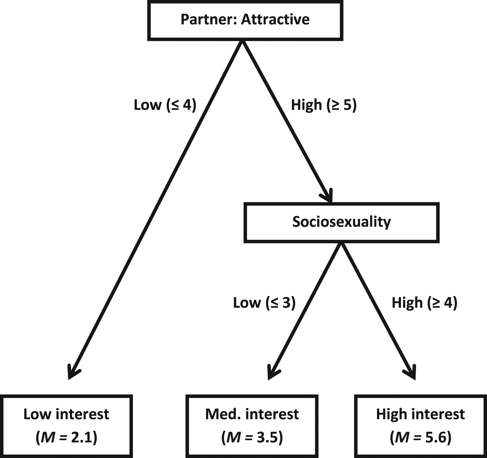
A single decision tree is likely to overfit a given dataset; random forests address this problem. The random forests approach first builds a decision tree from a random subset of predictors and 2/3 of the cases (rather than the entire dataset). Next, it tests the tree’s overall predictive power on the remaining 1/3 of cases that were not used to construct the original decision tree; this latter set of cases is called the “out of bag” (OOB) sample. Then, these steps are repeated across several thousand trees. Predictors and splits are likely to differ from one tree to the next, but given that repeatedly testing predictors in different subsamples of a common dataset is an especially robust way of culling a set of predictors (see simulations in Breiman, 2001a), predictors (and combinations thereof) that truly matter will end up being retained across many trees. Finally, the results are averaged together, and the output reveals (a) how accurately the model could predict the dependent measure (across the several thousand trees) and (b) which predictors reliably made contributions to the model. Again, given that decision trees themselves capture any main effects, nonlinear effects, and interactions among predictors that happen to be present, random forests should capture these effects, too. Importantly, however, there is no single final output tree that depicts how all the variables fit together in a single algorithm. Rather, the output is a forest, in which some types of trees are more common than others.
Each model was conducted using the “randomForest” package for R using tuning parameters from Joel et al. (2017, 2020; ntree = 5000, mtry = p/3); we used median imputation for all missing values among the predictors, and we used a “regression” task because the romantic interest DVs are continuous. Also, the widely used “VSURF” package for R determines which specific predictors should be retained by drawing from the permutation-based importance values that are commonly assigned to each predictor in a random forests model (Genuer et al., 2015). VSURF cuts predictors sequentially across three steps: threshold → interpretation → prediction. That is, at the threshold step, VSURF is very liberal with the variables it retains: it only cuts variables that never contribute to the model. Then, at the interpretation (i.e., moderate) step, VSURF retains the especially important predictors, even if they are redundant with each other. Finally, at the prediction (i.e., conservative) step, VSURF increases the standards further and retains until only the most important and non-redundant predictors. Colloquially, the threshold (liberal) step only drops variables that are primarily noise, the prediction (conservative) step tries to use as few predictors as possible, and the interpretation (moderate) step falls in between. Our stage 1 preregistration emphasized the interpretation (moderate) step, and therefore, only variables retained at the interpretation step were examined in stage 2 of the analysis plan. However, for completeness, we present overall model performance for all three steps in the stage 1 Results section below.
The common output measure of model performance with random forests is the coefficient of determination (R2; i.e., percentage of variance accounted for); higher values of R2 indicate that the model had greater predictive accuracy (Rosenbusch et al., 2021). 3 In response to reviewer feedback, we also conducted a set of k-fold cross-validation random forests analyses (i.e., 10 times repeated 10-fold cross validation, or 10 × 10-fold CV) based off of the procedures of Stachl, Pargent et al. (2020). K-fold cross validation is a technique that (in the case of 10 × 10-fold CV) iteratively trains the random forests model on 90% of the dataset and tests it on the remaining 10%. The difference between OOB and k-fold is that OOB uses all cases across (in this case) all 5000 trees, whereas k-fold reports the R2 achieved by applying the trained model to the test (i.e., 10%) sample that was set aside.
There is some debate about whether OOB random forest procedures operate “with cross-validation being performed along the way” (Hastie et al., 2009, p. 593), or whether OOB random forests overfit the data relative to k-fold cross-validation (Stachl, Pargent et al., 2020); we report both approaches in stage 1. Regardless, the k-fold R2 has a major advantage over OOB R2: It is possible to conduct hypothesis tests that compare k-fold R2 values from different models using a t-test with a correction that addresses the dependence across the CV models (Bouckaert & Frank, 2004; Stachl, Au et al., 2020). We also report the results of these t-tests below.
In the current study, the predictors are the individual-difference reports (159 measures) and target-specific reports (30 measures), and each case is a participant’s romantic interest dependent measure (initial report, peak, final report, or slope) regarding one potential partner (N = 1,065 in the primary analysis). 4 The full dataset with N = 7,179 rows has three levels: time (level 1) nested within target (level 2) nested within participant (level 3). Our four romantic interest DVs aggregate across the lowest level (time) to produce a dataset with N = 1,065 rows. Nevertheless, this dataset still has two levels (target nested within participant), and random forests and the VSURF predictor selection algorithm do not make adjustments for multilevel structures. As a robustness check against overfitting, we also conducted random forests models only on each participants’ first target (N = 208; see the Supplemental Materials).
We conducted models with three different batches of predictors: (a) all the individual-difference reports, (b) all the target-specific reports, and (c) all individual-difference reports and target-specific reports combined (i.e., a “batch” incremental validity approach; Großmann et al., 2019; Joel et al., 2020). Intuitively, it seems as though adding all the individual-difference reports to the target-specific reports (i.e., analysis c) would surely predict more variance than the models containing the target-specific reports alone (i.e., analysis b). But for the predicted variance to be higher in analysis (c), one or both of two conditions must be true: Either the target-specific reports must be moderated by individual differences (i.e., the perceiver × target moderation account of compatibility), or the individual differences must exert direct effects on romantic interest that are completely unmediated by any target-specific reports (i.e., the direct-influence model). If the addition of individual-difference reports accounts for approximately the same variance as the target-specific reports alone, then neither of these conditions is likely to hold, implying that individual-differences affect romantic interest primarily via mediated expression rather than direct influence or moderation (Joel et al., 2020). Simulations in the Supplemental Materials demonstrate that Random Forest models can recover moderation effects using the batch incremental validity approach: The addition of individual-difference reports indeed predicts more variance than target-specific reports alone if moderation effects are built into the data. 5 Also, it is worth noting that polygenic studies use decision trees and random forests to successfully document gene × gene interactions using a similar approach (Bureau et al., 2005; McKinney et al., 2006; Pociot et al., 2004).
Results
Basic descriptive information
First, given that datasets examining early relationship development over time are extremely rare, we conducted some basic descriptive analyses on the romantic interest dependent measure. Figure 2 depicts the average romantic interest values across all N = 1,065 potential partners at each of the ten time points. Critically, time = 1 is the romantic interest report when the potential partner entered the dataset (i.e., the initial report), not (necessarily) wave 1 of the study itself (i.e., the first week of October). In other words, only potential partners who were nominated on the first longitudinal questionnaire could possibly reach the time = 10 data point (hence, the error bars are wider for the later time points), and potential partners who were nominated on the tenth and final longitudinal questionnaire could only contribute to the time = 1 data point. Generally speaking, when participants nominated potential partners for the first time (time = 1), their romantic interest ratings were considerably higher than at subsequent time points. Three weeks after a potential partner was nominated (time = 2), the participant’s romantic interest had already dropped by nearly a full scale point. Romantic interest in potential partners over time. Note. Romantic interest was reported on a 1-7 rating scale. Time = 1 is the wave that the participant first nominated the potential partner. Ns for each time point are included at the base of each bar. Bars = +/− 1 SE.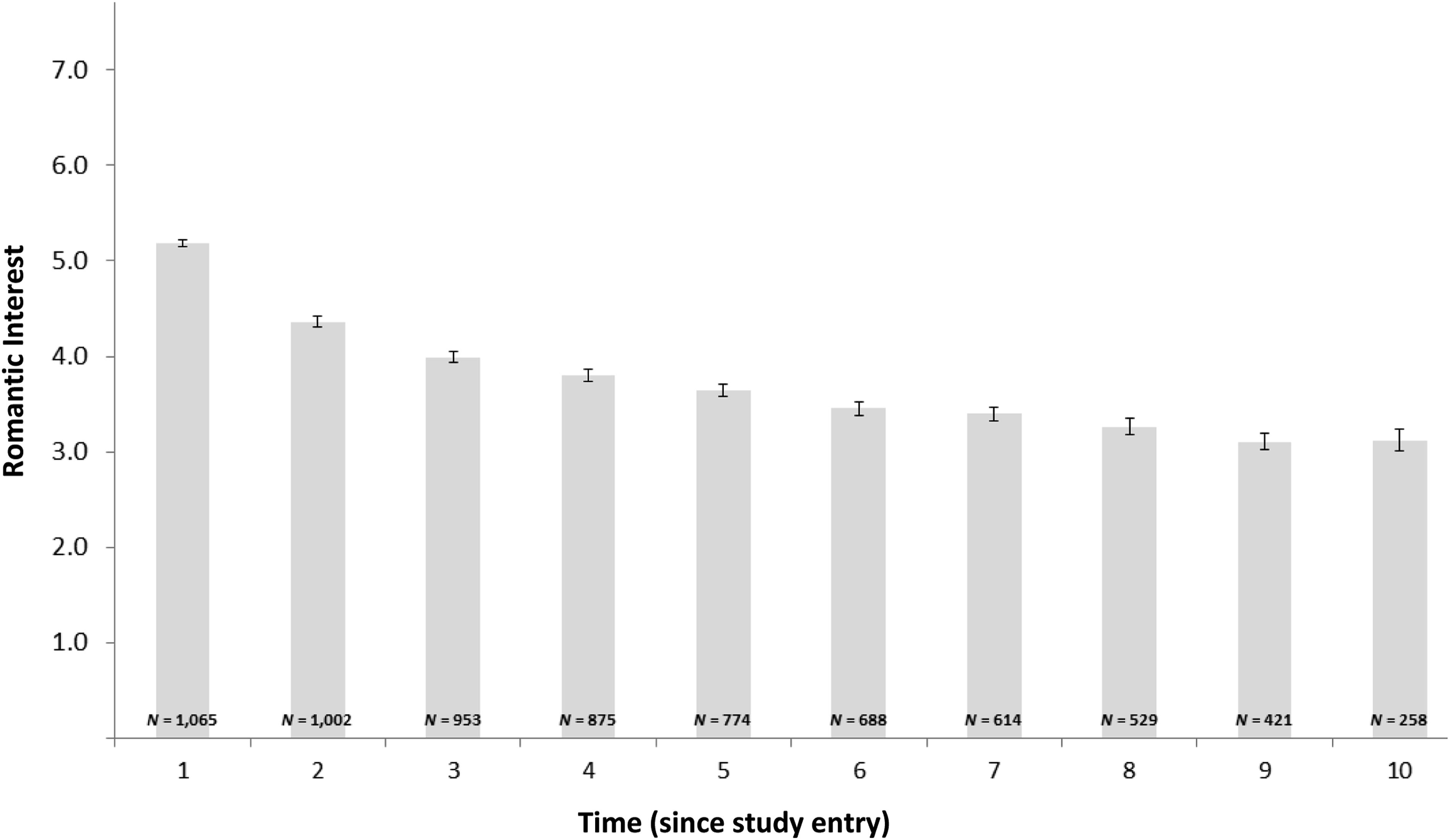
Figure 3 contains spaghetti plots of this descriptive data over time, along with the average romantic interest values (i.e., the thick black line) corresponding to each time point. Panel A depicts the 112 dating relationships used in the dating subset analyses in the Supplemental Materials, whereas Panel B depicts 112 potential partners who were both (a) randomly selected from the “first” potential partners that participants nominated (i.e., the very first potential partner who came to mind on the first longitudinal questionnaire) and (b) never casual or serious dating partners at any point. Romantic interest for the relationships depicted in Panel A is higher than those depicted in Panel B, especially at the later time points (i.e., the d values below the x-axis in Figure 3 get larger on average with time). Relatedly, the spaghetti plots suggest that participants’ romantic interest in partners they will date (at some point) often start high and remain high over time (Panel A), whereas romantic interest in the random set of never-dated potential partners start high but decline precipitously at some point (Panel B). In other words, it may be hard to “carry a torch” for someone over many months unless you actually get to date them at some point. Spaghetti plots for dated (a) and never-dated (b) potential partners. Note. Romantic interest was reported on a 1-7 rating scale. Time = 1 is the wave that the participant first nominated the potential partner. Panel A depicts N = 112 potential partners that the participant casually or seriously dated at some point; Panel B depicts N = 112 random potential partners nominated at the first wave of the study but whom participants never dated at any point. Values below the x-axis refer to effect size d between Panels A and B at each point. Bars = +/− 1 SE.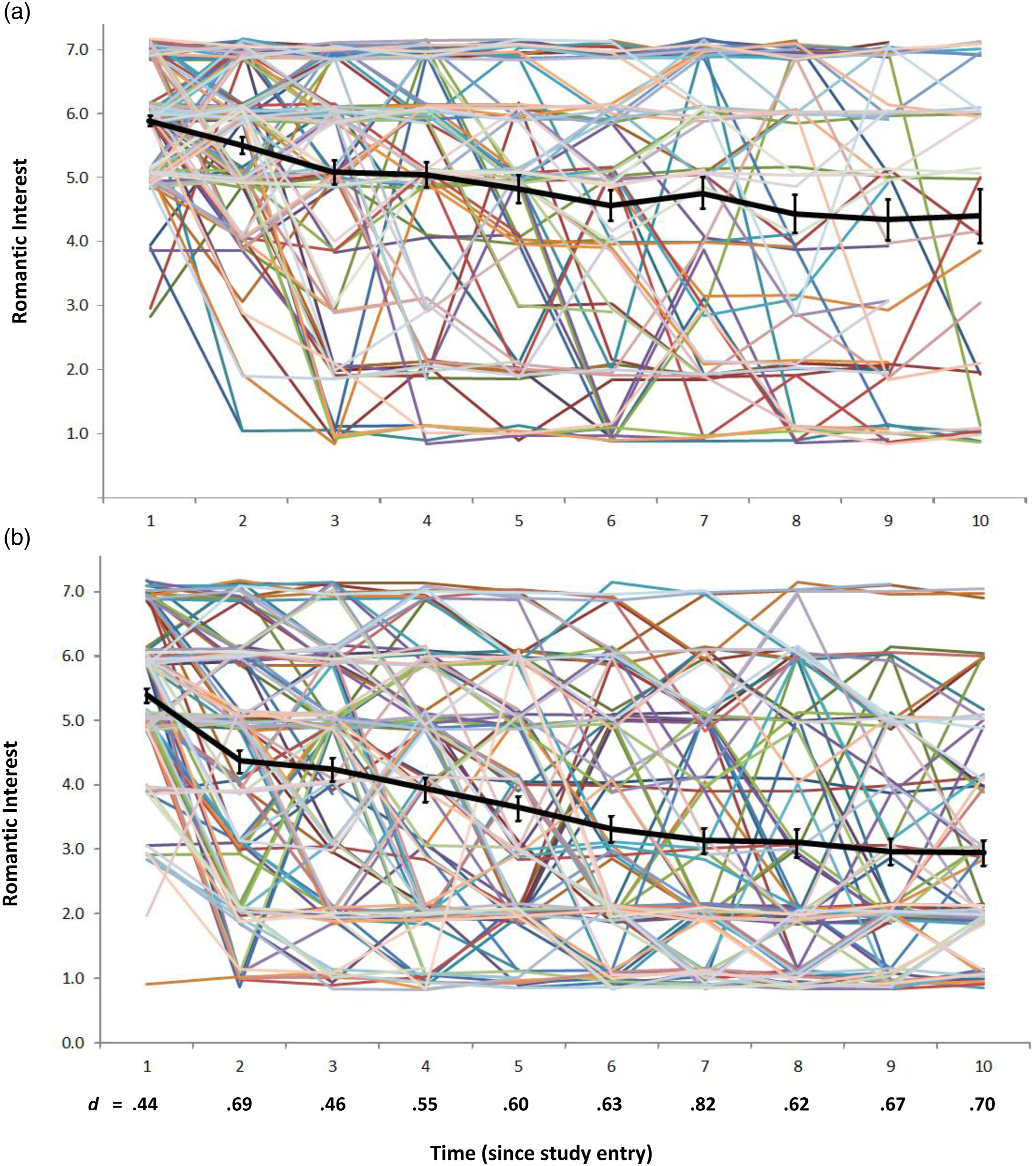
Figure 4 contains histograms of the number of participants who (a) casually/seriously dated partners during the course of the study (i.e., anyone above 0 comprises the dating subsample; Panel A) and (b) reported engaging in “any romantic physical contact (kissing or other sexual activities)” with a potential partner (Panel B). (This is a target-specific item; see Appendix B.) The subset of participants who engaged in romantic physical contact (n = 139, or 67% of the total sample of participants) is nearly double the number who reported having a dating relationship (n = 79, or 38%). Also, participants reported having physical contact with n = 317 different targets on 1,400 (out of 7,179) reports. Thus, the number of physical contact partners is approximately triple the number of dating partners (n = 112), which is consistent with the suggestion that the average college student’s pool of hookup partners is considerably larger than their pool of dating partners (Wade, 2017). (Not surprisingly, nearly all of the dating partners were included in the pool of physical contact partners; n = 106, or 94.5%.) Nevertheless, most participants did not have romantic physical contact with a great variety of partners over 7 months (i.e., 87.5% had 0–3 physical contact partners). Histograms of total dating (a) and physical contact (b) partners. Note. Panel A depicts the number of casual/serious dating partners that each participant reported during the course of the study. Panel B depicts the number of partners with whom a given partner had romantic physical contact (kissing or other sexual activities) during the course of the study. Total N = 208 for each panel; percentages within a panel add up to 100%.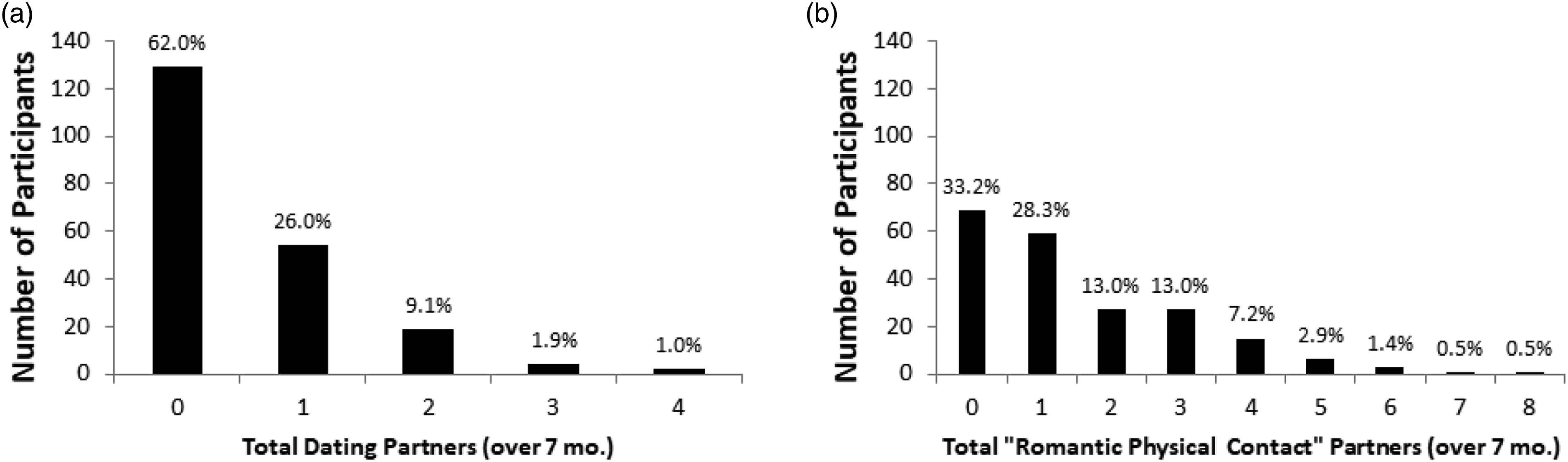
Machine learning with random forests
Associations among the four romantic interest DVs.
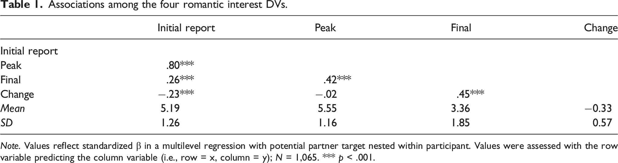
Note. Values reflect standardized β in a multilevel regression with potential partner target nested within participant. Values were assessed with the row variable predicting the column variable (i.e., row = x, column = y); N = 1,065. *** p < .001.
Machine Learning Analyses Predicting Romantic Interest in the Full Sample.
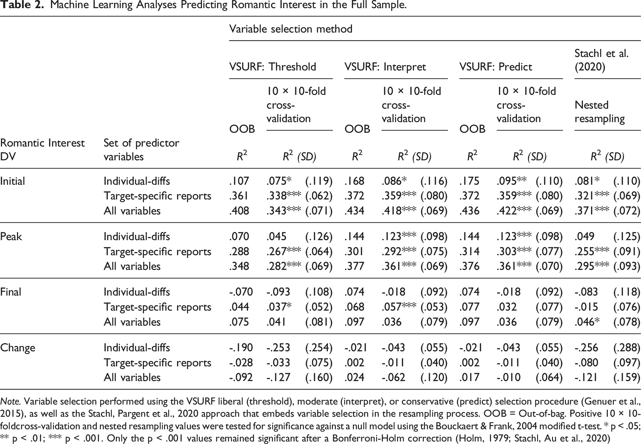
Note. Variable selection performed using the VSURF liberal (threshold), moderate (interpret), or conservative (predict) selection procedure (Genuer et al., 2015), as well as the Stachl, Pargent et al., 2020 approach that embeds variable selection in the resampling process. OOB = Out-of-bag. Positive 10 × 10-foldcross-validation and nested resampling values were tested for significance against a null model using the Bouckaert & Frank, 2004 modified t-test. * p < .05;** p < .01; *** p < .001. Only the p < .001 values remained significant after a Bonferroni‐Holm correction (Holm, 1979; Stachl, Au et al., 2020)
A seventh, nested resampling approach (labeled Stachl et al., 2020) does not use VSURF but rather embeds variable selection in the resampling process—that is, the included variables in each iteration of the model are selected based only on their performance in the (90%) training dataset, not the (remaining 10%) test set. (This procedure simply selects the 10 variables that correlate most highly with DV at each iteration.) 6
Across all seven analyses in Table 2, individual differences (by themselves) predicted a meaningful amount of variance for the initial report (11.3%; range 7.5%–16.5%) and peak (10.0%; range 4.5%–14.4%) DVs. Target-specific reports performed well for the initial report (35.5%; range 32.1%–37.2%) and peak (28.9%; range 25.5%–31.4%) DVs. Generally speaking, the OOB R2 values were higher than the equivalent k-fold R2 values by 3.4%, and higher than the Stachl et al. (2020) nested resampling R2 values by 7.9%; these analyses suggest that the OOB procedure may have overfit the data to a modest extent. Nevertheless, the relative pattern of R2 values was the same across all analyses.
Machine learning analyses predicting romantic interest in the full sample using 5-fold CV.
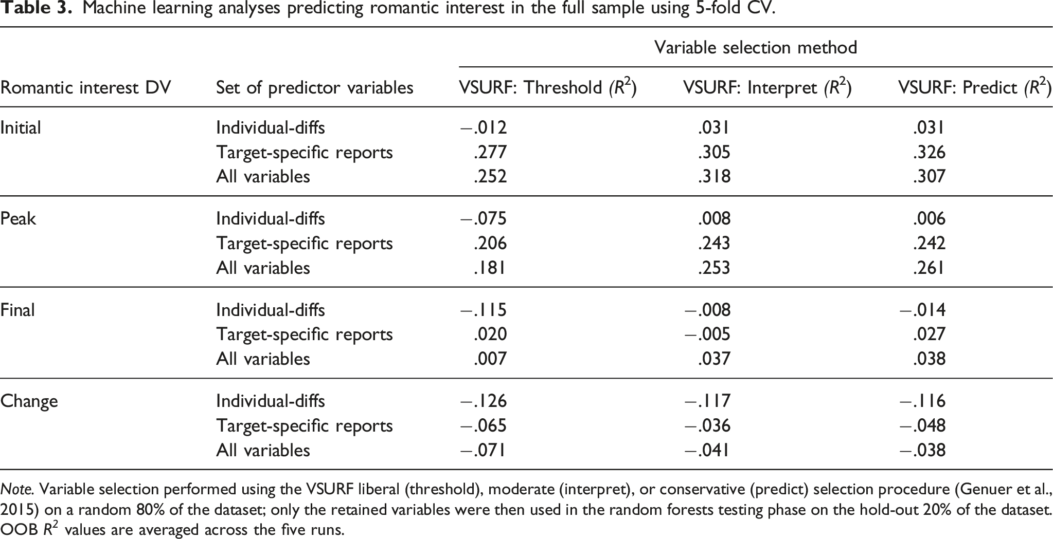
Note. Variable selection performed using the VSURF liberal (threshold), moderate (interpret), or conservative (predict) selection procedure (Genuer et al., 2015) on a random 80% of the dataset; only the retained variables were then used in the random forests testing phase on the hold-out 20% of the dataset. OOB R 2 values are averaged across the five runs.
Significance tests corresponding to k-fold and nested resampling R2 values in Table 2.
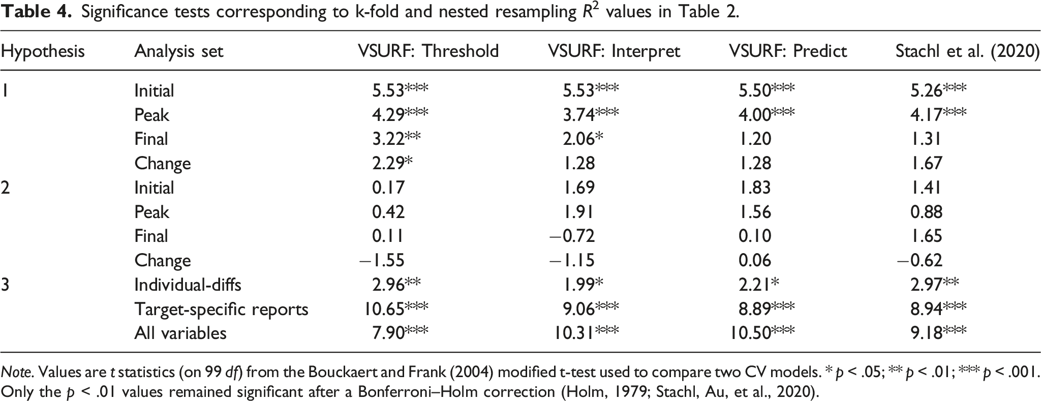
Note. Values are t statistics (on 99 df) from the Bouckaert and Frank (2004) modified t-test used to compare two CV models. * p < .05; ** p < .01; *** p < .001. Only the p < .01 values remained significant after a Bonferroni–Holm correction (Holm, 1979; Stachl, Au, et al., 2020).
Hypothesis 2: The second pre-registered analysis showed that the addition of individual-difference reports only modestly increased the amount of variance that could be predicted, as illustrated by the fact that the “all variables” rows in Tables 2 and 3 were nearly the same as the “target-specific reports” rows. On average, across the initial, peak, and final report DVs, this difference was 2.9% (initial DV difference = 3.2%, peak difference = 3.8%, final report difference = 1.7%), and the difference was actually negative for the change DV (−2.1%). 0 of the 16 hypothesis tests comparing a given pair of “all variables” and “target-specific reports” analysis was significant (Table 4). Conceptually, these findings suggest that effects of individual-difference reports on romantic interest in potential partners could be mediated by target-specific reports (i.e., mediated expression models), but they are not especially likely to exert direct effects or to moderate the effects of target-specific reports (or else individual-differences would have predicted more variance when added to the models). These findings are also consistent with Joel et al. (2020), which found that individual-difference reports predicted ∼1% of the variance above and beyond target-specific reports, depending on the analysis. Notably, it might be meaningful that the estimate here is a bit higher (2.9%), even if no comparison was significant.
Hypothesis 3: The third pre-registered analysis showed that the models predicting the initial report performed better than the models predicting the final report, as illustrated by the fact that the rows for the “initial report” in Tables 2 and 3 are considerably higher than the parallel rows for the “final report” (Δ = 24.5% on average); all 12 relevant hypothesis tests were significant (Table 4). Indeed, our ability to predict final report romantic interest was fairly poor overall; no analysis exceeded 10%, and many R2 values were negative, which indicates that the model performed no better (and might have performed notably worse) than guessing the grand mean. By way of comparison, Joel et al. (2020) was generally able to predict 10-20% of relationship satisfaction using similar individual-difference reports and target-specific variables M = 14 months later. It may be easier to predict the future of established relationships (as in Joel et al., 2020) than it is to predict the future of potential partnerships.
Hypothesis 4: The fourth pre-registered analysis showed that it was challenging to predict slope effects, as evidenced by the fact that none of the change analyses succeeded in predicting more than 2.4% of the variance, and most estimates were negative. Values in Joel et al. (2020) also tended to be quite low (i.e., 5% of the variance or less). It may not be possible to predict the extent to which someone experiences an increase or a decrease in romantic interest in a potential partner from variables assessed at baseline (i.e., prior to or concurrent with the moment that the participant first reports on the partner). It is also possible that the variance in the change DV is too small to be predictable at all (Table 1).
Discussion
For stage 1 of our analysis plan, we used random forests to examine the extent to which people’s romantic interest in potential partners is predictable. All four preregistered hypotheses received support. Although these hypotheses were not severe tests of a single existing theory and might strike many readers as intuitively obvious (Mayo, 1991), they provide estimates of the relative importance of different classes of variables that will facilitate our ability to develop robust mathematically informed models (e.g., Kenny, 2004; MacInnis & Page-Gould, 2015). Also, these data tested a generalizability question: Do the findings of Joel et al. (2020) apply to this (rarely studied) early relationship development context? The results suggest that the answer is “yes,” and because the hypotheses were preregistered and the data themselves did not inform the hypotheses, we can adjust our confidence in the generalizability of these findings upward (Ledgerwood, 2018). The findings were consistent regardless of whether we examined the full sample or the dating subset (see Supplemental Materials), although estimates in the dating subset proved more variable given the smaller sample size.
First, for the initial and peak DVs, both individual differences (7% across Tables 2 and 3) and target-specific reports (31%) predicted a meaningful amount of variance in romantic interest. Also, the difference between these two estimates is consistent with a common assumption among close relationships researchers that measures of the relationship itself provide the best insights into the nature of human mating (Van Lange, 2010). This finding is also consistent with many theories in the close relationships literature positing that individual differences play a more distal role than people’s private perceptions of their partners in affecting relational outcomes (e.g., Karney & Bradbury, 1995; Rusbult et al., 2001). Of course, some proportion of this effect could be due to common method variance (e.g., participants completed the target-specific measures and the romantic interest DV at the same time; Podsakoff et al., 2003). In fact, the methodological and conceptual similarity among these target-specific measures means that scholars sometimes consider the target-specific measures that we used as predictors to be outcome measures (Fletcher et al., 2000b). Future measurement work should endeavor to create a detailed and complete psychometric taxonomy of target-specific measures to ensure that close-relationships scholars are not routinely predicting an outcome with itself (Flake & Fried, 2020; Wang & Eastwick, 2020).
Second, in the preregistered analyses, the addition of individual-difference reports did not reliably contribute beyond target-specific reports in predicting romantic interest. A best reasonable estimate of the incremental predictive effect of all individual differences was ∼3%; this value is higher than the estimate obtained by Joel et al. (2020) of 1%, although importantly, none of these analyses were significant and this 3% value should be viewed tentatively. If individual-difference constructs (a) exerted unmediated direct influence on romantic interest or (b) reliably moderated the effects of target-specific reports (e.g., the meta-theoretical perceiver × target moderation account of compatibility), then the addition of individual-difference reports should presumably have predicted additional variance. Instead, mediated expression models—whereby individual-difference reports operate as distal constructs that influence romantic interest through target-specific constructs—may prove more robust than the direct influence and perceiver × target moderation models. Critically, however, we did not have access to any of the target’s self-reports. As a consequence, we were only able to test one conceptualization of the perceiver × target moderation account of compatibility in this study, whereas earlier work on speed-dating (Joel et al., 2017) and established relationships (Großmann et al., 2019; Joel et al., 2020) was able to test a second conceptualization that incorporates interactions between the perceiver and target’s self-reported variables. In addition, no machine learning study to date has tested the especially provocative possibility that the perceiver × target moderation account of compatibility has predictive power when incorporating the target’s actual behavior (e.g., agreeable people like targets who give compliments). Such tests would be especially worthwhile, whether the results support the perceiver × target moderation account or not.
Third, baseline romantic interest proved to be more predictable than later romantic interest from individual differences and target-specific variables also reported at baseline. Interestingly, final report romantic interest was more difficult to predict than in established relationship contexts (Joel et al., 2020), a finding we did not anticipate. It is plausible that most of these potential partnerships did not have a strong dyadic foundation (e.g., no sustained reciprocal interest yet), and so the target-specific constructs that we assessed might prove relatively ephemeral—rapidly shifting for the better or worse as these relationships evolve.
Fourth and finally, the models were unable to predict the extent to which romantic interest increased versus decreased over the subsequent waves. It might seem obviously true that baseline measures could not predict slopes over time, but published studies commonly report such effects in established relationship contexts (e.g., Impett et al., 2008; McNulty et al., 2021, 2013; Murray et al., 2011; Valentine et al., 2020), and they follow from theories positing that incompatibilities are latent early in relationships and primarily reveal themselves with time (Felmlee, 1995). Future research will need to examine why the current findings revealed a different conclusion, and it is possible that we did not assess enough time points for most potential partners to reliably detect change.
Machine learning can illuminate which outcomes are predictable and which sets of measures are useful in making those predictions. But traditional multilevel modeling approaches can provide additional insights into the nature of the associations between successful predictors and a given outcome while appropriately accounting for the nested structure of the dataset. (The inability of VSURF to account for nesting may mean that the Table 2 estimates are optimistic overall, and indeed, supplemental analyses in Table S9 using only the participant’s first target produced somewhat lower estimates; Δ R2 = −.019 on average.) In addition, even though the findings for hypothesis 2 suggested that individual-difference reports were unlikely to moderate the effects of target-specific reports on romantic interest, it would be sensible to directly test influential moderation hypotheses of this form. Although the meta-theoretical perceiver × target moderation account of compatibility can take a wide variety of forms, our particular measures put us in a strong position to test one of these theories especially precisely: ideal partner preference-matching. Thus, we preregistered a second stage to our analysis plan (after conducting the preregistered analyses reported above) that specifically set out to (a) plot the effects of specific meaningful predictors and (b) test theories of ideal partner preference-matching.
Stage 2
The form of perceiver × target compatibility that has received the most consistent research attention over the past two decades is ideal partner preference-matching (Eastwick et al., 2019a; Fletcher et al., 1999; 2020). Ideal partner preference-matching refers to the hypothesis that people who profess a strong ideal for a particular attribute in a partner (e.g., the individual-difference report “My ideal partner is attractive”) should be especially likely to positively evaluate partners who possess the attribute (e.g., the target-specific report “_____ is attractive”). Ideal-partner preference matching is a paradigmatic illustration of the meta-theoretical perceiver × target account of compatibility (i.e., perceivers like x will fit with targets like y), and it further presumes that participants themselves can articulate (as conveyed by their stated ideals) the sort of partner with whom they will fit.
There are several strong analytic techniques available for testing this hypothesis (Eastwick et al., 2019a). One is the pattern metric, which predicts romantic interest from the Fisher z-transformed within-person correlation between (a) all available ideal partner preference measures (in this case, ideals for 14 traits) and (b) the participant’s perception of the partner on those same (14) traits. This approach addresses whether people are especially likely to experience romantic interest for partners who possess traits that match their overall pattern of ideals. Critically, participants’ ratings on ideals and traits include some amount of general positivity, and the psychometric solution to this “normative desirability confound” requires that the researcher mean-center all items before calculating the within-person correlation (i.e., the corrected pattern metric; Rogers et al., 2018; Wood & Furr, 2016). A second is the level metric, which predicts romantic interest one trait at a time from each Ideal × Trait interaction (controlling for the main effect of the ideal and the trait). This approach addresses whether people with strong ideals for a particular trait are especially likely to experience romantic interest in partners to the extent that those partners possess that trait. Our stage 2 analysis plan included preregistered tests of both of the corrected pattern metric and level metric approaches; the ideal standards model generates the hypothesis that these tests will produce positive effects sizes (on average) that are significantly and meaningfully different from zero.
A reviewer recommended we also try a third approach—response surface analysis (RSA; Humberg et al., 2019). RSA specifically examines the evaluative consequences of congruence (i.e., similarity) between the ideal value and trait value, one trait at a time (like the level metric). Whereas the level metric tests a model where ideals serve as weights that affect how strongly a given attribute predicts a positive evaluation of a partner, RSA tests a model where ideals serve as templates whereby positive evaluations follow from the extent that ideals and traits are close together rather than far apart (Conroy-Beam, 2021). The RSA analyses did not support the ideal partner preference-matching hypothesis and are included in the Supplemental Materials.
Method
We used the same dataset described in stage 1 (i.e., participants, procedure, and materials).
Analysis plan stage 2: Specific predictors
We used multilevel modeling to depict (one-at-a-time) each of the meaningful predictors that was retained at the interpretation step of VSURF in stage 1. We preregistered that we would focus on the interpretation (i.e., moderate) selection step, as it seemed like a balanced decision criterion that would yield an informative set of predictors, most of which would have made meaningful (rather than tiny) contributions. In Table 2, 7 of the 12 interpretation step nested resampling analyses were significantly different from zero; in these 7 analyses, 34 different predictors (12 individual-difference reports, 22 target-specific reports) were retained in the model at least once (see Appendices A and B). We used multilevel modeling to conduct the following analysis on each of these 34 predictors, one at a time
Finally, we conducted analyses examining ideal partner preference-matching using (a) 14 ideal-partner preference items reported on the in-lab questionnaire (e.g., physical attractiveness, dependable, exciting, and optimistic) and (b) the 14 corresponding partner-trait items reported at the first wave the potential partner entered the database. Using equation (1), we conducted both the (a) corrected pattern metric (1 analysis) and (b) level metric (14 analyses) tests as described in Eastwick et al. (2019a). Specifically, for the corrected pattern metric analysis, “predictor” was a Fisher-z scored version of the within-person correlation between the 14 ideal ratings and the 14 partner-trait ratings after sample-mean centering all 28 items. For the level metric analysis, “predictor” was the Ideal × Trait interaction (after sample-standardizing the ideal and trait); the main effects of ideal and trait were also included in this analysis (as well as the Ideal × Time, Ideal × Time2, Trait × Time, and Trait × Time2 terms).
Results
Successful predictors in equation (1): Preregistered analyses
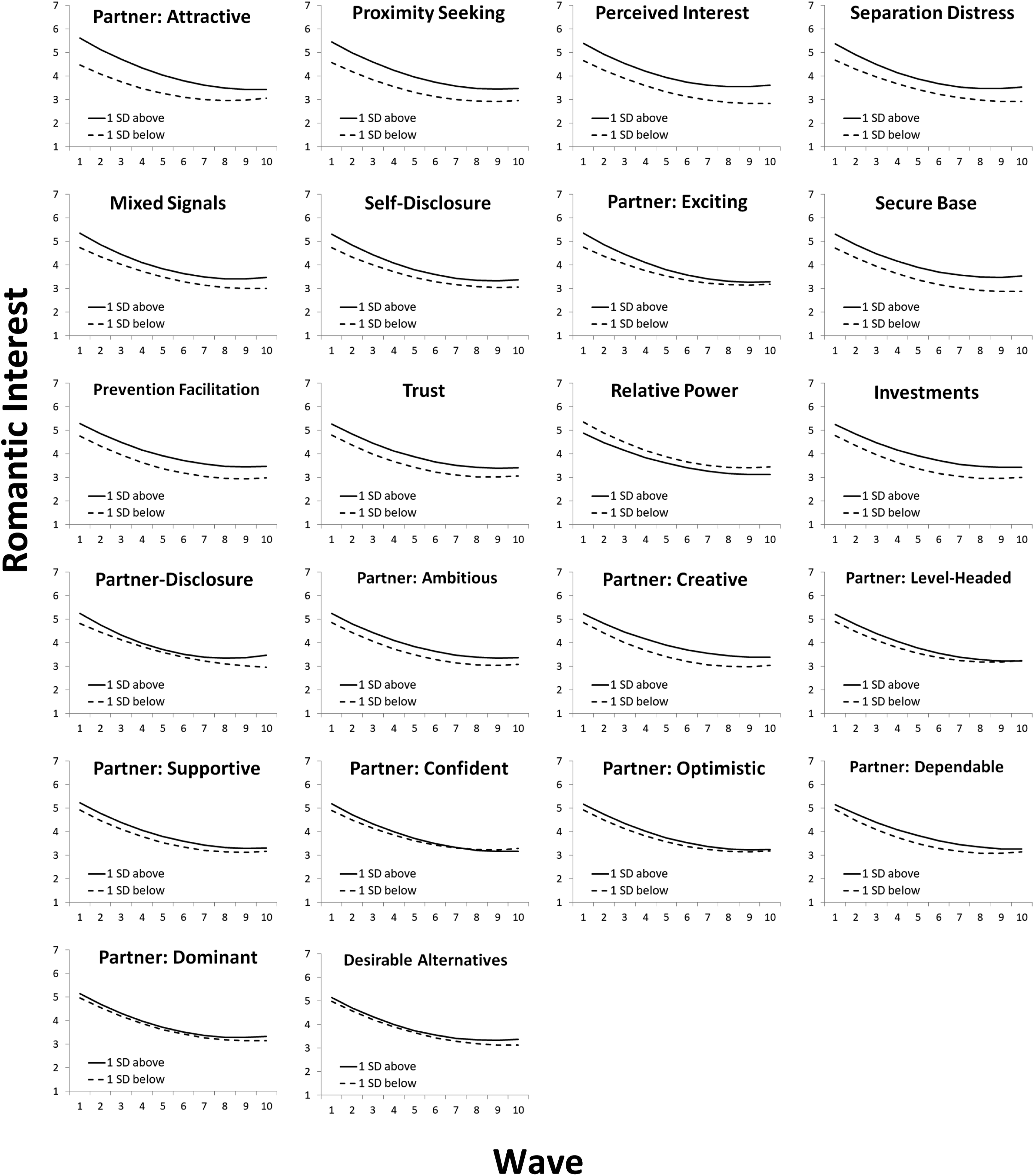
The 34 predictors that were retained in every statistically significant nested resampling random forests analysis (at the interpret VSURF step) are presented in Figure 5 (the 12 individual-difference predictors) and Figure 6 (the 22 target-specific predictors). Individual difference variables had four opportunities to serve as predictors (twice by themselves and twice in combination with target-specific variables), and target-specific variables had five opportunities to serve as predictors (twice by themselves and three times in combination with individual difference variables). The panels within each figure are sorted by the (absolute value of) the β
1
effect size. Successful individual-difference predictors. Note. Equation (1) results for the 12 individual-difference predictors that contributed to the significant nested resampling random forests models in stage 1 (Table 2). Predictors are sorted in the order of the magnitude of the β
1
(wave = 1) effect size.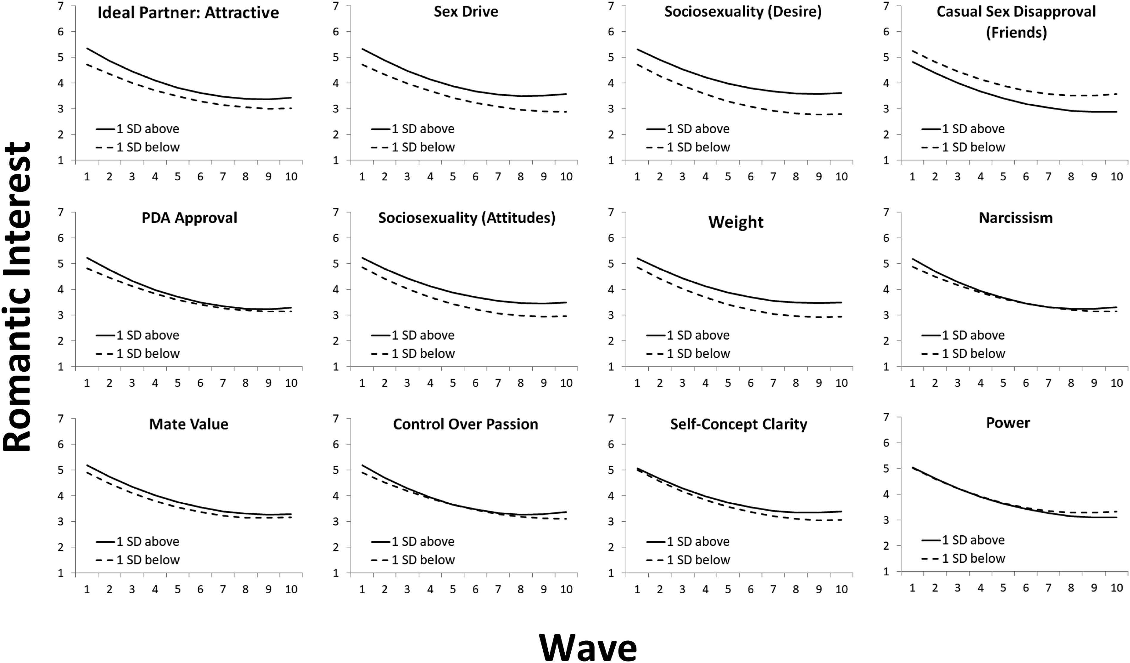
Equation (1) results for individual-differences predictors.
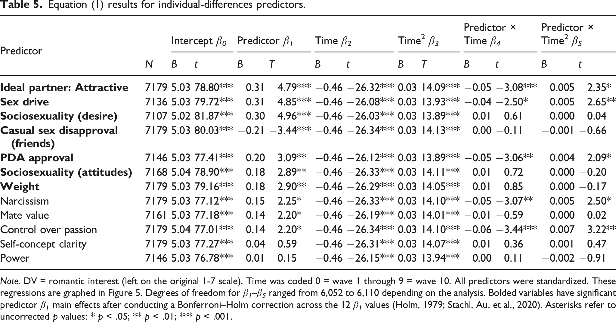
Note. DV = romantic interest (left on the original 1-7 scale). Time was coded 0 = wave 1 through 9 = wave 10. All predictors were standardized. These regressions are graphed in Figure 5. Degrees of freedom for β 1 –β 5 ranged from 6,052 to 6,110 depending on the analysis. Bolded variables have significant predictor β 1 main effects after conducting a Bonferroni–Holm correction across the 12 β 1 values (Holm, 1979; Stachl, Au, et al., 2020). Asterisks refer to uncorrected p values: * p < .05; ** p < .01; *** p < .001.
Equation (1) results for target-specific predictors.
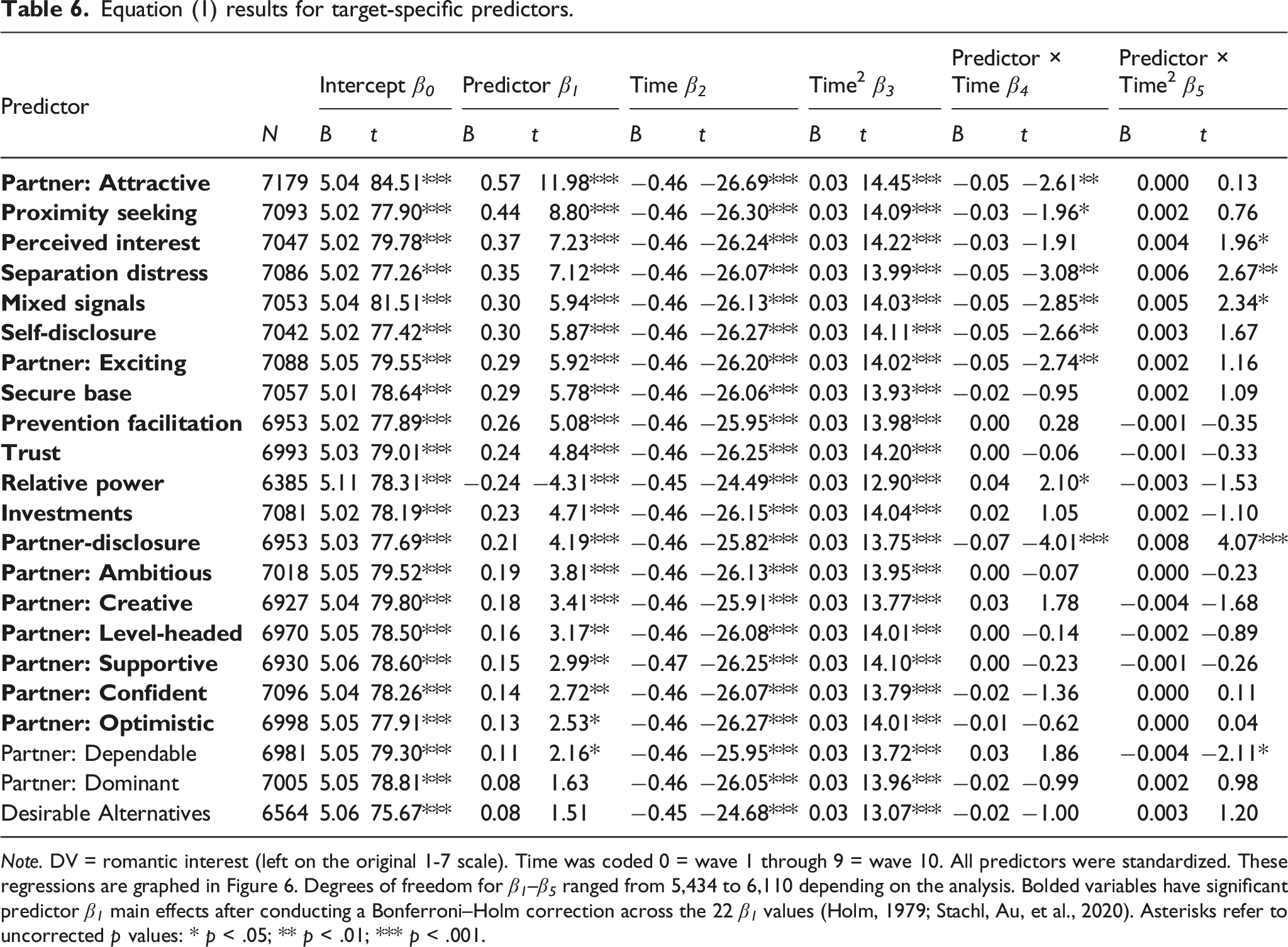
Note. DV = romantic interest (left on the original 1-7 scale). Time was coded 0 = wave 1 through 9 = wave 10. All predictors were standardized. These regressions are graphed in Figure 6. Degrees of freedom for β 1 –β 5 ranged from 5,434 to 6,110 depending on the analysis. Bolded variables have significant predictor β 1 main effects after conducting a Bonferroni–Holm correction across the 22 β 1 values (Holm, 1979; Stachl, Au, et al., 2020). Asterisks refer to uncorrected p values: * p < .05; ** p < .01; *** p < .001.
In a multilevel model, data records that correspond to a missing predictor value will be excluded from analysis. In this portion of the study, although response data at the first level were complete (i.e., romantic interest reports), some participants had missing data for predictors at levels 2 (target) and 3 (participant). The results presented in Tables 5 and 6 are based on data for which a particular predictor was observed, and so the sample sizes differ across the results. To evaluate the sensitivity of these results to missing data, we used maximum likelihood (ML) estimation carried out using Mplus version 8.6 (Muthen & Muthen, 1998-2017) in which the predictors were assumed to be random and normally distributed variables (as opposed to being fixed in the first set of analyses). Thus, the two methods of estimation differ by their treatment of the missing data, as well as the distributional assumptions made about the predictors. In the Supplemental Materials, we reproduced Tables 5 and 6 using this alternative estimation method. Results did not appreciably differ: Across the two analyses, the β 1 estimates for the predictors differed by no more than .017 (Δ M = .005 across the two tables), and the correlation between the β 1 values within Table 5 and within Table 6 was r = .99 in both cases. The only difference was that the target-specific predictor Partner: Dependable was not significant according to the Bonferroni–Holm test in the analysis reported in Table 6, but it is significant in the maximum likelihood missing data analysis in Table S17.
Ideal partner preference-matching analyses (preregistered)
Corrected pattern metric
Level metric tests of ideal partner preference-matching.
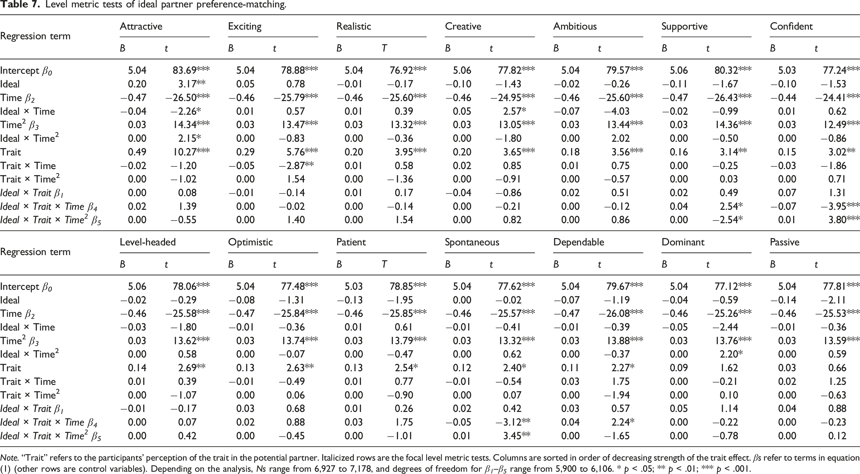
Note. “Trait” refers to the participants’ perception of the trait in the potential partner. Italicized rows are the focal level metric tests. Columns are sorted in order of decreasing strength of the trait effect. βs refer to terms in equation (1) (other rows are control variables). Depending on the analysis, Ns range from 6,927 to 7,178, and degrees of freedom for β 1 –β 5 range from 5,900 to 6,106. * p < .05; ** p < .01; *** p < .001.
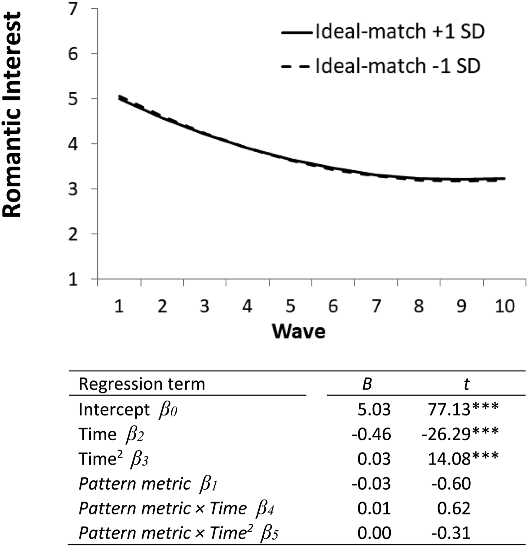
Ideal partner preference-matching over time (corrected pattern metric). Note. Italicized rows are the focal pattern metric tests. βs refer to terms in equation (1). N = 7,160; degrees of freedom for β 1 –β 5 = 6,095. *** p < .001.
Level metric
Table 7 presents the results of all 14 level metric tests, sorted (from left to right) by the strength of the main effect of the trait. That is, attractiveness had the strongest predictive effect on participants’ romantic interest (B = .49; approximately half a romantic interest-scale point with every SD of attractiveness), whereas passiveness had the weakest effect (B = .03). These traits effects can be conceptualized as the strength of the functional (i.e., revealed) preference for the trait in the full sample of participants (Ledgerwood et al., 2018); how strongly does a given trait predict participants’ romantic interest judgments, on average? All traits exhibited significant positive predictive effects except for dominance and passiveness.
The Ideal × Trait interactions test the predictive validity of ideal partner preference-matching: That is, does a trait predict romantic interest more strongly for people who ideally say they want the trait? There were zero (out of 14) significant Ideal × Trait interactions (average β 1 = .02 in Table 7), revealing no evidence that participants who expressed strong (vs. weak) ideals for a given attribute were especially likely to express romantic interest in potential partners who possessed the attribute. For slope effects, 2 of 14 level metric effects were significant and positive and 2 of 14 were significant and negative; average β 4 = .001. For curvilinear effects, 2 of 14 level metric effects were significant and positive and 1 of 14 was significant and negative; average β 5 = .001. In summary, ideal partner preference-matching effects were extremely small and typically no different from zero, and the significant effects that did emerge did not seem to be systematically positive versus negative in direction. (Analyses using the broader Fletcher et al., 1999, warmth/trustworthiness, and vitality/attractiveness constructs also revealed no support for ideal partner preference-matching; see the Supplemental Materials.)
Additional ideal partner preference analyses (exploratory)
In this section, we report four additional analytic approaches that some prior studies have used to garner evidence for ideal partner preference-matching.
Functional-summarized preference correlations
We also conducted the “functional-summarized preference correlation” variant of the level metric analysis used in some prior studies (also called a stated-revealed preference correlation; Brumbaugh & Wood, 2013; Eastwick & Smith, 2018; Wood & Brumbaugh, 2009). This analysis first requires that the researcher calculates a within-person slope (i.e., a personal regression β) that captures the within-person association (calculated across targets) between a given attribute and romantic interest for each participant; these slopes represent each participant’s functional preference for a given attribute (i.e., the extent to which the attribute inspired romantic interest for the participant across all targets; Ledgerwood et al., 2018). Then, we calculated the simple (between-persons) correlation of these functional preference values with the ideal partner preference for that attribute as reported on the intake questionnaire (i.e., also called a summarized preference; Ledgerwood et al., 2018). Summarized-functional preference correlations in prior work have tended to be moderately sized in contexts where participants rate photographs (e.g., r = ∼.20; Brumbaugh & Wood, 2013; Wood & Brumbaugh, 2009) and near-zero when participants rate initial attraction partners (r = ∼.03; Eastwick & Finkel, 2008b). The present analysis is the first assessment of functional-summarized preference correlations beyond initial attraction.
Functional-summarized preference correlations.
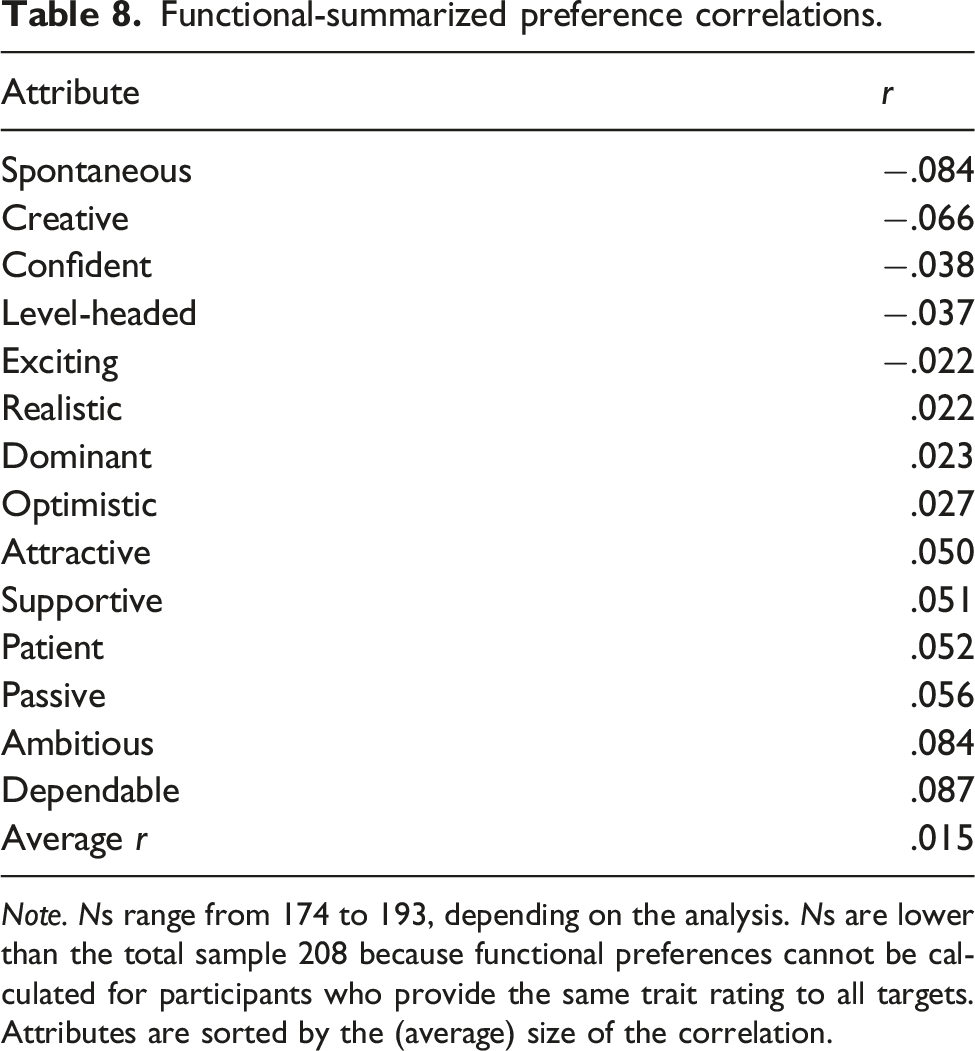
Note. Ns range from 174 to 193, depending on the analysis. Ns are lower than the total sample 208 because functional preferences cannot be calculated for participants who provide the same trait rating to all targets. Attributes are sorted by the (average) size of the correlation.
Scholars occasionally draw inferences about ideal partner preference matching by examining whether sex differences in summarized preferences match sex differences in functional preferences (Eastwick & Finkel, 2008b; Li et al., 2013). In other words, given that men say they care about attractiveness more than women (i.e., summarized preferences), does attractiveness actually predict men’s romantic interest more strongly than women’s romantic interest (i.e., functional preferences)? With respect to summarized preferences: Of the 14 ideal partner preference items, men gave significantly higher ratings than women to attractiveness, t(206) = 2.81, p = .005, d = .39, and women gave higher ratings than men to supportive, t(206) = −5.25, p < .001, d = .74; ambitious/driven, t(206) = −4.85, p < .001, d = .68; dominant, t(206) = −4.34, p < .001, d = .62; dependable, t(206) = −3.60, p < .001, d = .50; and confident, t(206) = −2.52, p = .012, d = .35. However, with respect to functional preferences, men and women did not differ in their functional preferences (i.e., personal regression βs) for any of these 6 traits, all ps > .315, ds < .15. (Indeed, men and women did not significantly differ in their functional preference for any of the 14 traits.)
Raw pattern metric
Ideal partner preference-matching (raw pattern metric).
Note. Italicized rows are the focal pattern metric tests. βs refer to terms in equation (1). N = 7,021; degrees of freedom for β 1 –β 5 = 5,983. * p < .05; *** p < .001.
Ideal-trait correlations
This final alternative approach omits the dependent measure (i.e., romantic interest) entirely and simply presents the correlations between the participant’s ideals and the participant’s perception of the partner’s traits (i.e., ideal-trait correlations). Sometimes, scholars conduct these analyses on samples where participants describe the traits of established relationship partners and presume that a positive correlation indicates that participants selected into these relationships because the partner matched the participant’s ideals (e.g., Conroy-Beam & Buss, 2016; Gerlach et al., 2019). However, this presumption is not valid: Myriad additional processes will produce positive ideal-trait correlations even in the absence of participants having (at some previous time) selected the partner because the partner matched their ideals (e.g., “perceiver effects” such that people who profess an ideal for particular trait also “see” that trait in their social milieu; Eastwick et al., 2019a). Nevertheless, we present these estimates here to be comprehensive.
Ideal-trait correlations.
Note. Attributes are sorted by the (average) size of the ideal-trait standardized beta (β). Depending on the analysis, Ns range from 1,019 to 1,064, and degrees of freedom range from 811 to 856. ** p < .01; *** p < .001.
Discussion
Stage 2 of our analysis plan used a common multilevel modeling approach to the study of early relationship development over time. First, we analyzed and plotted (one at a time) all of the predictors that were retained (at least once) by our machine learning models in stage 1. For individual-difference predictors, conceptualizing an ideal partner as attractive, sex drive, and sociosexuality exhibited the strongest predictive effects on romantic interest. For the target-specific predictors, several of the predictors were substantial, such as perceiving the potential partner (at study entry) to have positive qualities (e.g., attractive and exciting) and other variables associated with the activation of the normative attachment system (e.g., proximity seeking, separation distress, and secure base; Tancredy & Fraley, 2006). People also reported more romantic interest when they felt the potential partner was interested in them and also when they received mixed signals from the partner, which is consistent with Tennov’s (1979) classic perspective that romantic infatuation is often inspired by a blend of hope (i.e., “I think they are into me”) and uncertainty (i.e., “I get mixed signals about whether they are into me”).
Findings for hypothesis 2 in the machine learning component of the study (i.e., stage 1) suggested that individual-difference reports were unlikely to moderate target-specific reports. We tested this possibility more directly by examining one popular hypothesis of this form: ideal partner preference-matching. The two clearest analytic techniques (i.e., the corrected pattern metric, the level metric) revealed no evidence for ideal partner preference-matching; participants were no more or less likely to report romantic interest in potential partners who matched versus mismatched their ideals, in either the full sample (presented here) or the dating subsample (see the Supplemental Materials). The response surface analyses in the Supplemental Materials also revealed no support for a congruence hypothesis.
It is illustrative that the individual-difference with the strongest main effect to emerge from the random forest models was the ideal preference for an attractive partner, and the target-specific variable with the strongest main effect was the perception that the partner is attractive. These same two main effects can also be seen in the first (Attractive) column of Table 7, in the “Ideal” (B = .20) and “Trait” (B = .49) rows. These two constructs indeed matter. But they did not interact, as anticipated by the ideal standards model (i.e., the level-metric test); people with high ideals for attractiveness did not place more weight on their perception that a partner is attractive. The variables simply exerted main effects.
Importantly, the raw pattern metric did reveal positive effects, which suggests that prior studies using this approach (e.g., Eastwick et al., 2011) might have found evidence for ideal partner preference-matching because of the normative desirability confound—a statistical artifact (Wood & Furr, 2016). Ideal-trait correlations were strong and positive, which supports the suggestion that these correlations are caused by processes other than ideal partner preference matching (e.g., perceiver effects; Rau et al., 2021). In general, our failure to find support for ideal partner preference-matching is consistent with the machine learning findings from stage 1 (and from Großmann et al., 2019 and Joel et al., 2020): Moderation effects of individual-difference reports (i.e., perceiver × target accounts of compatibility) may be very small when used to predict romantic evaluations. Critically, however, we did not assess status/resources traits in this study, and there is some evidence that ideal partner preference-matching effects are especially likely to emerge for those traits in particular (Fletcher et al., 2020). If it turns out that ideal partner preference-matching effects emerge robustly for the status/resources dimension but not the other dimensions (or other perceiver × target accounts of compatibility), explanations for such a pattern would require significant new theory development.
General discussion
This study examined early relationship development longitudinally—one of the first studies of its kind. An exceptional feature of the dataset is that a participant’s relationship with a given potential partner did not ever need to “turn into something” to be included. Rather, the participant merely had to experience a modicum of romantic interest in the partner at some point during a 7-month period. Thus, this design provides a window into the nature of single individuals’ rising and falling romantic pursuits over time, and it captured both the (small) set of potential partners that ultimately became dating relationships and the (large) set that fizzled out.
Core findings
These analyses provide insights into the types of constructs and processes that are more or less influential in early relationship development. Individual differences (e.g., sex drive and sociosexuality) collectively predicted a modest amount of the variance in people’s initial report and peak romantic interest, although target-specific reports (e.g., perceptions of positive qualities, attachment features) predicted a greater amount (H1). Perceiver × target moderation accounts of compatibility generally performed weakly, predicting at best 3% of the variance in the aggregate (H2) and revealing no support in the specific tests of ideal partner-preference matching that we conducted in stage 2. Also, predictors of final report romantic interest were modest relative to predictors of initial report interest (H3), and predictors of change in romantic interest were nonexistent (H4).
The basic descriptive data help illuminate some key base rates with respect to early relationship development. At the person level, relationship formation was a common experience, albeit far from ubiquitous. Specifically, 38% of participants ended up dating at least one person casually or seriously over the 7-month period. These values seem consistent with Campbell et al. (2016) and Gerlach et al. (2019)—two of the few other prospective studies of singles—who reported that 39% and 34% (respectively) of participants formed a relationship over a 5-month period. In contrast, relationship formation at the relationship level was far less common: In the current study, only 11% of the potential partners would eventually become casual or serious dating partners. These values are compatible with those in Machia et al. (2020), who reported that 15% of friends-with-benefits relationships transitioned to a romantic relationship over the course of a year. These low percentages would likely drop even further if we had managed to track relationships from the moment two people met: The likelihood that a person will ultimately form a relationship with any of the 10–12 strangers they meet at a speed-dating event is approximately 5%, which amounts to <1% per stranger (Asendorpf et al., 2011; Eastwick, 2019). It will take considerably more intensive tracking efforts to understand what these survival curves look like over the full time course of early-relationship development (Joel & MacDonald, 2021).
Prior work has suggested that the normative trajectory of romantic interest over an entire relationship resembles an arc that rises and falls (Eastwick et al., 2018, 2019b). Intriguingly, the spaghetti plots in Figure 3 (i.e., the potential partners that never became relationships) do not resemble arcs on average—they start in the moderate range and typically decline from that point. There are several possible explanations for this pattern. One possibility is that rising and falling arcs describe dating and sexual relationships that survive long enough for something mutual to happen, whereas most “one-way” romantic interests flicker and disappear. A second possibility is that this survey design was too coarse to capture the rise of the arc: That is, perhaps romantic interest rose over the course of an initial conversation or two and had already peaked for most participants when the survey link arrived in their inbox weeks later. A third possibility is that the design of the study unintentionally encouraged participants to wait until they were especially confident that someone had strong romantic potential before nominating him/her, and thus, the downward slide reflects inevitable regression to the mean. To differentiate among these possibilities, we would need to recruit potential partners from an initial encounter, regardless of initial interest level, and then follow them intensively over the coming days, weeks, and months. Future studies should be designed with these considerations in mind.
Finally, the current data speak to the nature of the hookup culture on college campuses (Garcia et al., 2012; Wade, 2017)—or at least on one college campus. On the one hand, the current data indicate that the circle of partners with whom participants had sexual contact is wider than (and also subsumes) the circle they casually or seriously dated; these students seem more inclined to have sexual contact than to use the “dating” label. On the other hand, sexual contact was a positive predictor of romantic interest (albeit a small one; see Appendix B), which suggests that hooking up might serve as a gateway to a more intimate relationship, on average. Future longitudinal research on hookups should be sure to track information on the specific partners with whom participants are hooking up. Otherwise, numbers can be spun into something quite dramatic (our 208 participants hooked up 1,400 times!) when in fact they reflect something a bit more mundane (participants had only M = 1.5 hookup partners over a period of 7 months, which means they tended to hook up with the same person multiple times).
Theoretical implications
Most of the variables assessed in the current study were derived from existing theories and models of close relationships. In terms of individual differences, sociosexuality exerted a moderately positive main effect on romantic interest, which potentially explains why people higher in sociosexuality eventually acquire more casual and committed romantic relationships—they may simply be more amorous in early relationship contexts (Eastwick et al., 2019b; Penke & Asendorpf, 2008). Also, the main effect of the ideal preference for an attractive partner supports models that posit a motivational function for high ideals (i.e., the projection process documented by Murray et al., 1996). There was an average difference between men’s (M = 4.42) and women’s (M = 3.80) romantic interest values, t(206) = 5.24, p < .001, d = .73, which is consistent with evolutionary models of sex differences in romantic eagerness (Buss & Schmitt, 1993; Fletcher et al., 2014). However, the gender variable was never retained by VSURF at the interpretation step, which suggests that the effect of gender on romantic interest was likely distal to other factors. In other words, the sex-differentiated variables that were retained by the random forests models (e.g., sex drive, sociosexuality, and perceiving the partner to be attractive) likely fully mediated the effect of gender (e.g., Conley et al., 2011; Eastwick & Smith, 2018). Many other individual differences that commonly exert robust effects in established relationships (e.g., attachment anxiety, self-esteem, and implicit theories) were not selected by the random forest models; perhaps the individual-differences components of these theories do not generalize well to early relationship development.
Among the target-specific variables that tended to emerge, those that assessed dyadic communication processes (e.g., perceived interest, mixed signals, and self-disclosure) generally tended to reveal robust effects, as anticipated by many classic models of relationship formation (Altman & Taylor, 1973; Knapp, 1978; Tennov, 1979). Also, several of the normative components of attachment theory performed extremely well (e.g., proximity seeking, separation distress, and secure base), which suggests that the activation of the attachment system is a promising early sign in many fledging relationships (Eastwick & Finkel, 2008a; Heffernan et al., 2012). Target-specific perceptions of positive traits performed well, especially the traits that fit within the vitality/attractiveness construct (e.g., attractive and exciting), which is theorized to be central to relationship initiation (Fletcher et al., 2014). Nevertheless, perceptions of traits did not emerge as often as the more dyad-centered constructs on the whole.
The tests of hypothesis 2 were a central theoretical contribution of the current study. These tests revealed that individual differences predicted little (if any) variance in the machine learning models above and beyond target-specific predictors. This finding is consistent with an underlying process in which target-specific predictors mediate the effects of individual differences, not unlike the classic conceptualization of “complete mediation” whereby the effect of the distal predictor is reduced to zero by the inclusion of the mediator (Baron & Kenny, 1986). In fact, the findings for hypothesis 2 make the novel conceptual assertion that there may be many undiscovered target-specific mediators that explain why sex drive and sociosexuality (i.e., two of the stronger individual differences that emerged) predict romantic interest. However, the hypothesis 2 effects are not consistent with a process where individual differences exert direct effects or moderate the effects of target-specific predictors on romantic evaluations. Along with three other machine learning studies (Großmann et al., 2019, and Joel et al., 2017, 2020), there is now accumulating evidence that perceiver × target accounts of compatibility are unlikely to successfully explain the prominence of relationship effects in romantic evaluations (Eastwick & Hunt, 2014; Kenny, 2020).
These machine learning studies thus serve a crucial role in the service of theory development, even though machine learning itself works through an atheoretical process of testing variables at random until an optimal solution emerges. Mate Evaluation Theory (MET) is one theory that has been constructed (in part) from prior machine learning efforts (Eastwick et al., in press). MET seeks to explain how it can simultaneously be true that (a) relationship effects constitute the largest percentage of variance in romantic evaluations (Kenny, 2020) and (b) relationship effects largely cannot be explained by appealing to perceiver × target interactions. MET explains these seemingly incompatible pieces of evidence by positing not one but two conceptually distinct sources of relationship effects. The first source (called the “feature lens”) refers to individual differences in the way certain perceivers evaluate targets based on the targets’ features (e.g., traits). This source includes any account suggesting that “certain people evaluate certain other people positively” and encompasses all forms of the meta-theoretical perceiver × target account of compatibility (e.g., ideal preference-matching, similarity-matching, and mate-value matching; Chopik & Lucas, 2019; Van Scheppingen et al., 2019; Sparks et al., 2020; Tidwell et al., 2013; Watson et al., 2004). The second source (called the “target-specific lens”) refers to history, narrative, “microculture,” idioms, rituals, and other forms of personal knowledge that are bound to one and only one relationship (Bell et al., 1987; Dunleavy & Booth-Butterfield, 2009; Finkel, 2020; Garcia-Rada et al., 2018; Harris et al., 2014; Rossignac-Milon et al., 2021; Rossignac-Milon & Higgins, 2018; Weigel & Murray, 2000). This source captures effects that are not generalizable to other similar perceivers and targets, including events and disclosures that partners experience with each other that are not available to other perceivers. In other words, Lawrence might evaluate Issa uniquely positively not because she matches his ideals or because they have similar interests (i.e., feature lens), but instead because of the way she supported his career aspirations at a critical point in his life or because he enjoys how she counters his teasing with her own (i.e., target-specific lens).
This approach suggests that the reason that compatibility effects are difficult to predict is because the information that determines relationship effects varies idiosyncratically not simply from person to person, but also from relationship to relationship. That is, compatibility primarily emerges as a consequence of the narrative history and idioms that are created within a particular relationship that does not generalize to other relationships (Bell et al., 1987; Garcia-Rada et al., 2018; Harris et al., 2014; Rossignac-Milon & Higgins, 2018). This perspective generates the prediction that accounting for relationship effects will require that scholars tailor items in a way that incorporates the relationship’s own narrative structure (Adler et al., 2017; Bühler & Dunlop, 2019; Sparks et al., 2020). For example, it may be the case that Lawrence feels uniquely positive about Issa because of the way they tease each other—and he would feel less positive if that dynamic changed—but that particular standard would not apply to his past or future relationships. Future work that better allows participants to define for themselves what events or patterns make a given relationships uniquely positive or negative may be critical for predicting compatibility effects, especially if the classic perceiver × target approach continues to reveal extremely small effect sizes.
Strengths and limitations
This article provides an intensive look at the romantic lives of young single people as they considered different potential romantic partners. No previous studies have incorporated into the study of early relationship development repeated longitudinal measurements of multiple targets, and so the trajectories that we documented here fill a crucial gap in the close relationships literature (Eastwick et al., 2019b). Furthermore, we incorporated both machine learning approaches and traditional multilevel models in an attempt to balance concerns about overfitting (Yarkoni & Westfall, 2017) against the utility of presenting familiar growth curve models accounting for the nested structure of our data (Singer & Willett, 2003) that are most directly comparable to the existing literature. We preregistered our analysis plans in both stage 1 and stage 2 to establish a priori what we believed to be the most informative approach to addressing our primary research questions. Finally, this study illustrates how the study of singles (Pepping et al., 2018) can incorporate target-specific variables and constructs in their research; participants do not need to be in one exclusive romantic relationship to report on different romantic targets (for a polyamory example, see Moors et al., 2019).
This study also has a number of limitations that can be addressed by future research. First, as noted above, we did not capture participants’ romantic interest from the moment they met the potential partners. Doing so will be a very resource-intensive undertaking—perhaps requiring a consortium of scholars—especially if it proves generalizable that (a) only 40% of a sample of singles starts a new dating relationship in a ∼6-month period (as we found here) and (b) the odds of relationship formation with a stranger at the target-specific level are 1% or less (Asendorpf et al., 2011). 7
Second, we did not have access to objective measures of the nature of the interaction between the participant and the potential partner. Such constructs may have performed well, especially given that the interaction-focused (but participant-reported) measures were often retained by the random forests models. It is also possible that the perceiver × target account of compatibility would have received more support with such tests (e.g., perhaps agreeable people like potential partners who give compliments).
Third, we did not have access to the potential partners’ self-reported individual differences. These measures would have provided a cleaner comparison between the perceiver × target account of compatibility tested here—in which all variables were filtered through the participant’s own mind—and the one tested in Joel et al. (2020) that also incorporated such partner reports. Furthermore, it is interesting to consider that partner reports of individual differences predict a very small amount of variance (5% or less) in prior machine learning work on established relationships (Großmann et al., 2019; Joel et al., 2020), yet they predict much more variance in speed-dating contexts (e.g., 20–25%; Joel et al., 2017); it remains unclear which context is more comparable with early relationship development. 8
Fourth, our participants were all from a single college campus embedded within a WEIRD culture (Henrich et al., 2010). These findings may not generalize to cultures that are more restrictive of sexuality or relational mobility (Kito et al., 2017) or cultures with high levels of parent involvement (Gui, 2017).
Fifth, we used the random forests machine learning approach, which is an approach that trains each component of the model on 2/3 of the available dataset, then tests it on the remaining 1/3 of the dataset. That is, each tree is evaluated on its ability to predict the outcome variable in a subsample of data that were not used to fit that tree. We also used a k-fold cross-validation approach, which has the advantage of permitting null hypothesis significance testing (Stachl, Pargent et al., 2020). Although such resampling approaches help to avoid statistical overfitting issues (Yarkoni & Westfall, 2017), they do not speak to the generalizability of the findings in a way that collecting a new dataset would, particularly if that new study had different sample properties. The current study is but one dataset with one particular set of measures, and extensions to new datasets with new measures would be valuable.
Sixth and finally, we were only in a strong position to directly test one out of several possible perceiver × target accounts of compatibility (i.e., ideal partner-preference matching for traits). Other studies should directly test perceiver × target effects on the particular variables that are supposed to be especially central to similarity-attraction (e.g., attitudes and health behaviors; Bahns et al., 2017) and to mate-value (e.g., popularity and sociality; Fisher et al., 2008).
Conclusion
The data reported in this article suggest that early relationship development is a turbulent and volatile period in which different potential partners migrate in and out of people’s lives. Over the 7-month period of this study, all participants reported on multiple potential partners, and many would ultimately go on to form sexual or dating relationships—at least temporarily. Our machine learning approach revealed that a wide variety of target-specific and individual-difference variables helped to predict why romantic interest was higher for some of these potential partners than others. Also, we used both macro (i.e., the machine learning batch incremental validity strategy) and micro (i.e., the level and corrected pattern metric tests) approaches to test perceiver × target accounts of compatibility. Our lack of support for these accounts reinforces the need for scholars to develop and test new explanations for the prominence of compatibility in human attraction that goes beyond fit between different stable features of perceivers and targets. These endeavors will be critical in explaining why some relationships form—and why some of them eventually thrive—whereas many others do not.
Supplemental Material
sj-pdf-1-erp-10.1177_08902070221085877 - Supplemental Material for Predicting romantic interest during early relationship development: A preregistered investigation using machine learning
Supplemental Material, sj-pdf-1-erp-10.1177_08902070221085877 for Predicting romantic interest during early relationship development: A preregistered investigation using machine learning by Paul W Eastwick, Samantha Joel, Kathleen L Carswell, Daniel C Molden, Eli J Finkel and Shelley A Blozis in European Journal of Personality
Footnotes
Acknowledgments
We wish to thank Dr. Karisa Young Lee, who managed this project.
Declaration of conflicting interests
The author(s) declared no potential conflicts of interest with respect to the research, authorship, and/or publication of this article.
Funding
The author(s) disclosed receipt of the following financial support for the research, authorship, and/or publication of this article: This research was supported by NSF Grant BCS-0951571 awarded to Daniel C. Molden and a UC Davis Small Research Grant awarded to Paul W. Eastwick.
Data accessibility statement
Supplemental Material
Supplemental material for this article is available online.
Notes
Appendix A Individual-difference Report Variables (159) Used in Machine Learning Analyses
| Construct | Example item | # of items | Citation (for established scales) | Retained by random forests (interp step)? | |
|---|---|---|---|---|---|
| Full (of 4) | Dating (of 1) | ||||
| Age | How old are you? | 1 | 0 | 0 | |
| Agreeableness | I sympathize with others’ feelings. | 4 | Donnellan et al., 2006 | 0 | 0 |
| Approach goals | In relationships, I generally try to enhance the bonding and intimacy in my romantic relationship. | 4 | Impett et al., 2008 | 0 | 0 |
| Assessment | I often critique work done by myself or others. | 12 | Kruglanski et al., 2000 | 0 | 0 |
| Attachment anxiety | I worry about being abandoned. | 18 | Brennan et al., 1998 | 0 | 0 |
| Attachment avoidance | I prefer not to show a partner how I feel deep down. | 18 | Brennan et al., 1998 | 0 | 1 |
| Attractive resistance | If an attractive person (of my preferred sex) approached me sexually, it would be hard to resist, no matter how well I knew him or her. | 1 | Bailey et al., 1994 | 0 | 0 |
| Avoidance goals | In relationships, I generally try to avoid getting embarrassed, betrayed, or hurt by my romantic partner. | 4 | Impett et al., 2008 | 0 | 0 |
| Behavioral activation (drive) | I go out of my way to get things I want. | 4 | Carver & White, 1994 | 0 | 1 |
| Behavioral activation (fun) | I am always willing to try something new if I think it will be fun. | 4 | Carver & White, 1994 | 0 | 0 |
| Behavioral activation (reward) | When I am doing well at something, I love to keep at it. | 5 | Carver & White, 1994 | 0 | 0 |
| Behavioral inhibition | I feel pretty worried or upset when I think or know somebody is angry with me. | 7 | Carver & White, 1994 | 0 | 0 |
| Capitalization | I usually respond enthusiastically when loved-ones tell me about something good that has happened to them. | 2 | Gable et al., 2004 | 0 | 0 |
| Casual sex disapproval (family) | My family would disapprove of me having casual sex. | 1 | 1 | 0 | |
| Casual sex disapproval (friends) | My friends would disapprove of me having casual sex. | 1 | 0 | 0 | |
| Cheating | If I could maintain a long-term relationship with one partner while having sexual relations outside of my relationship, I would do so. | 1 | Landolt et al., 1995 | 0 | 0 |
| Collective self-construal | When I am in a group, it often feels to me like that group is an important part of who I am. | 2 | Cross et al., 2000 | 0 | 0 |
| Conscientiousness | I get chores done right away. | 4 | Donnellan et al., 2006 | 0 | 0 |
| Control over passion | No matter how hard they try, people can’t really change the sexual attraction/desire or passion they feel toward someone. | 4 | 1 | 0 | |
| Depression | I did not feel like eating; my appetite was poor. | 20 | Radloff, 1977 | 0 | 0 |
| Desperation | I sometimes feel as though I would date anyone who is interested in me. | 2 | 0 | 0 | |
| Destiny beliefs | Potential relationship partners are either compatible or they are not. | 11 | Knee, 1998 | 0 | 0 |
| Education (father) | What is the highest education level achieved by your father? [some high school…graduate degree] | 1 | 0 | 0 | |
| Education (mother) | What is the highest education level achieved by your mother? [some high school…graduate degree] | 1 | 0 | 0 | |
| Extraversion | I am the life of the party. | 4 | Donnellan et al., 2006 | 0 | 0 |
| Forgiveness | I tend to forgive quickly when someone hurts my feelings | 3 | Brown, 2003 | 0 | 0 |
| Friend value | I am a desirable friend. | 4 | 0 | 0 | |
| Friendship comfort | In general, I am comfortable expressing my interest forming a friendship with someone. | 1 | 0 | 0 | |
| Friendship initiation | I usually initiate a friendship with someone rather than wait for that person to initiate. | 1 | 0 | 0 | |
| Friendship standards | I am very picky about my choice of friends. | 1 | 0 | 0 | |
| Gender | What is your gender? [male, female] | 1 | 0 | 0 | |
| Gender identity | I have many interests (e.g., hobbies, possible careers) which are not stereotypic of my gender. | 1 | 0 | 0 | |
| Growth beliefs | The ideal relationship develops gradually over time. | 11 | Knee, 1998 | 0 | 0 |
| Health (overall) | In general, would you say your health is [poor...excellent] | 1 | 0 | 0 | |
| Health (symptoms) | Migraine headache | 33 | Cohen & Hoberman, 1983 | 0 | 0 |
| Height | What is your height? | 1 | 0 | 0 | |
| Ideal friend: ambitious | Ambitious/Driven | 1 | 0 | 0 | |
| Ideal friend: attractive | Physically attractive | 1 | 0 | 0 | |
| Ideal friend: confident | Confident | 1 | 0 | 0 | |
| Ideal friend: creative | Creative | 1 | 0 | 0 | |
| Ideal friend: dependable | Dependable | 1 | 0 | 0 | |
| Ideal friend: dominant | Dominant | 1 | 0 | 0 | |
| Ideal friend: exciting | Exciting | 1 | 0 | 0 | |
| Ideal friend: level-headed | Level-headed | 1 | 0 | 0 | |
| Ideal friend: optimistic | Optimistic | 1 | 0 | 0 | |
| Ideal friend: passive | Passive | 1 | 0 | 0 | |
| Ideal friend: Patient | Patient | 1 | 0 | 0 | |
| Ideal friend: realistic | Realistic | 1 | 0 | 0 | |
| Ideal friend: spontaneous | Spontaneous | 1 | 0 | 0 | |
| Ideal friend: supportive | Supportive | 1 | 0 | 0 | |
| Ideal partner: ambitious | Ambitious/Driven | 1 | 0 | 0 | |
| Ideal partner: attractive | Physically attractive | 1 | 2 | 0 | |
| Ideal partner: confident | Confident | 1 | 0 | 0 | |
| Ideal partner: creative | Creative | 1 | 0 | 0 | |
| Ideal partner: dependable | Dependable | 1 | 0 | 0 | |
| Ideal partner: dominant | Dominant | 1 | 0 | 0 | |
| Ideal partner: exciting | Exciting | 1 | 0 | 0 | |
| Ideal partner: level-headed | Level-headed | 1 | 0 | 0 | |
| Ideal partner: optimistic | Optimistic | 1 | 0 | 0 | |
| Ideal partner: passive | Passive | 1 | 0 | 0 | |
| Ideal partner: patient | Patient | 1 | 0 | 0 | |
| Ideal partner: realistic | Realistic | 1 | 0 | 0 | |
| Ideal partner: spontaneous | Spontaneous | 1 | 0 | 0 | |
| Ideal partner: supportive | Supportive | 1 | 0 | 0 | |
| Impression management | I am a completely rational person. | 10 | Paulhus, 1984 | 0 | 0 |
| Income (household) | What is the approximate total income of the household in which you were primarily raised? | 1 | 0 | 0 | |
| Independence | My personal identity, independent of others, is very important to me. | 12 | Singelis, 1994 | 0 | 0 |
| Interdependence | I have respect for the authority figures with whom I interact. | 12 | Singelis, 1994 | 0 | 0 |
| Liberal | I endorse many aspects of liberal political ideology. | 2 | Eastwick et al., 2009 | 0 | 0 |
| Limerence | When I am romantically interested in someone, I often ruminate upon every word and gesture from our interactions. | 4 | Feeney & Noller, 1990 | 0 | 0 |
| Locomotion | I enjoy actively doing things, more than just watching and observing. | 12 | Kruglanski et al., 2000 | 0 | 1 |
| Loneliness | I lack companionship. | 3 | Hughes et al., 2004 | 0 | 0 |
| Long-term preference | I prefer a long term relationship with one partner. | 1 | Landolt et al., 1995 | 0 | 0 |
| Mate value | I am a desirable dating partner. | 5 | Landolt et al., 1995 | 3 | 0 |
| Naps | During the past month, how often have you taken naps during the day? [never…3+ times a week] | 1 | 0 | 0 | |
| Narcissism | I see myself as a good leader. | 8 | Ames et al., 2006 | 3 | 0 |
| Need to belong | I want other people to accept me. | 10 | Leary et al., 2013 | 0 | 0 |
| Neuroticism | I have frequent mood swings. | 4 | Donnellan et al., 2006 | 0 | 0 |
| Openness | I have a vivid imagination. | 4 | Donnellan et al., 2006 | 0 | 0 |
| Parental divorce | Are your parents divorced? [yes, no] | 1 | 0 | 0 | |
| Passion theories | If you lose sexual attraction for your partner, you will never recover it. | 10 | Carswell & Finkel, 2018 | 0 | 0 |
| PDA | It’s fine with me if others see me be physically affectionate towards romantic partners. | 4 | 2 | 0 | |
| Power | I can get people to listen to what I say. | 15 | Anderson et al., 2012 | 1 | 0 |
| Prevention focus | Growing up, I typically obeyed rules and regulations that were established by my parents. | 5 | Higgins et al., 2001 | 0 | 0 |
| Promotion focus | I have often accomplished things that got me “psyched” to work even harder. | 6 | Higgins et al., 2001 | 0 | 0 |
| Reciprocity (friend) | I tend to want to be friends with people whom I think want to be friends with me. | 2 | 0 | 0 | |
| Reciprocity (romantic) | I tend to be romantically interested in people who like me back. | 4 | 0 | 0 | |
| Rejection sensitivity (concern) | How concerned or anxious would you be over whether or not your friend would do this favor? | 8 | Downey & Feldman, 1996 | 0 | 0 |
| Rejection sensitivity (expectations) | I would expect that my parents would he/she would willingly do this favor for me. | 8 | Downey & Feldman, 1996 | 0 | 1 |
| Relational self-construal | When I feel very close to someone, it often feels to me like that person is an important part of who I am. | 2 | Cross et al., 2000 | 0 | 0 |
| Romantic comfort | In general, I am comfortable expressing my romantic interest to someone I am interested in. | 1 | 0 | 0 | |
| Romantic initiation | I usually initiate a dating or romantic relationship with someone rather than wait for that person to initiate. | 1 | 0 | 0 | |
| Romantic standards | I am very picky about my choice of romantic partners. | 1 | 0 | 0 | |
| R’ship goals: casual dates | Finding someone to date casually [yes, no] | 1 | 0 | 0 | |
| R’ship goals: casual friend | Developing new casual friendships [yes, no] | 1 | 0 | 0 | |
| R’ship goals: close friend | Developing new close friendships [yes, no] | 1 | 0 | 0 | |
| R’ship goals: serious | Finding a serious romantic relationship [yes, no] | 1 | 0 | 0 | |
| R’ship goals: short-term | Finding short-term romantic relationships (e.g., one-night sexual encounters or brief affairs) [yes, no] | 1 | 0 | 0 | |
| R’ships long-term | In considering possible romantic partners, I typically think about their “long-term” potential. | 1 | 0 | 0 | |
| R’ships serious | My romantic relationships are nearly always committed and serious. | 1 | 0 | 0 | |
| Self-concept clarity | In general, I have a clear sense of who I am and what I am. | 12 | Campbell et al., 1996 | 1 | 0 |
| Self-esteem | I feel that I am a person of worth, at least on an equal basis with others. | 10 | Rosenberg, 1965 | 0 | 0 |
| Self: ambitious | Ambitious/Driven | 1 | 0 | 0 | |
| Self: attractive | Physically attractive | 1 | 0 | 0 | |
| Self: confident | Confident | 1 | 0 | 0 | |
| Self: creative | Creative | 1 | 0 | 0 | |
| Self: dependable | Dependable | 1 | 0 | 0 | |
| Self: dominant | Dominant | 1 | 0 | 0 | |
| Self: exciting | Exciting | 1 | 0 | 0 | |
| Self: level-headed | Level-headed | 1 | 0 | 0 | |
| Self: optimistic | Optimistic | 1 | 0 | 0 | |
| Self: passive | Passive | 1 | 0 | 0 | |
| Self: patient | Patient | 1 | 0 | 0 | |
| Self: realistic | Realistic | 1 | 0 | 0 | |
| Self: spontaneous | Spontaneous | 1 | 0 | 0 | |
| Self: supportive | Supportive | 1 | 0 | 0 | |
| Self-control | I am good at resisting temptation. | 13 | Tangney et al., 2004 | 0 | 1 |
| Self-respect | I have a lot of respect for myself. | 3 | Kumashiro et al., 2002 | 0 | 0 |
| Sex drive | I have a strong sex drive. | 2 | 4 | 1 | |
| Sexual orientation | I am exclusively attracted to members of the opposite sex. | 1 | Eastwick et al., 2011 | 0 | 0 |
| Sleep quality | During the past month, would you rate your overall sleeping quality as [very bad…very good] | 1 | 0 | 0 | |
| Social anxiety | I find myself worrying that I won’t know what to say in social situations. | 19 | Mattick & Clarke, 1998 | 0 | 0 |
| Social desirability | I never regret my decisions. | 10 | Paulhus, 1984 | 0 | 0 |
| Sociosexuality (attitudes) | Sex without love is okay. | 3 | Penke & Asendorpf, 2008 | 2 | 0 |
| Sociosexuality (behaviors) | With how many different partners have you had sex (sexual intercourse) within the last 12 months? | 3 | Penke & Asendorpf, 2008 | 0 | 1 |
| Sociosexuality (desire) | How often do you have fantasies about having sex with someone with whom you do NOT have a committed romantic relationship? [never…several times per week] | 3 | Penke & Asendorpf, 2008 | 4 | 0 |
| Staying awake | During the past month, how often have you had trouble staying awake while driving, eating meals, etc. [never…3+ times a week] | 1 | 0 | 0 | |
| Stereotype awareness (general) | People generally do not expect women to do well in Math and Science courses. | 1 | 0 | 0 | |
| Stereotype awareness (specific) | My professors think that women will do not well in Math and Science courses. | 1 | 0 | 0 | |
| Stereotype endorsement | I do not expect women to do well in Math and Science courses. | 1 | 0 | 0 | |
| Subjective well-being | In most ways, my life is close to ideal. | 5 | Diener et al., 1985 | 0 | 0 |
| Values: achievement | Competence and success | 1 | Schwartz & Bilsky, 1987 | 0 | 0 |
| Values: authority | Respect for authority | 1 | Schwartz & Bilsky, 1987 | 0 | 0 |
| Values: avoid hurting partners | I go to great lengths to avoid hurting romantic partners. | 1 | 0 | 0 | |
| Values: benevolence | Enhancing the welfare of those close to me | 1 | Schwartz & Bilsky, 1987 | 0 | 0 |
| Values: casual sex | It is against my values to have casual sex. | 1 | 0 | 0 | |
| Values: compassion | Compassion | 1 | Schwartz & Bilsky, 1987 | 0 | 0 |
| Values: conformity | Meeting social expectations | 1 | Schwartz & Bilsky, 1987 | 0 | 0 |
| Values: fairness | Fairness | 1 | Schwartz & Bilsky, 1987 | 0 | 0 |
| Values: hedonism | Pleasure and self-gratification | 1 | Schwartz & Bilsky, 1987 | 0 | 0 |
| Values: love | Love | 1 | Schwartz & Bilsky, 1987 | 0 | 0 |
| Values: power | Status and prestige | 1 | Schwartz & Bilsky, 1987 | 0 | 0 |
| Values: purity | Purity | 1 | Schwartz & Bilsky, 1987 | 0 | 0 |
| Values: relationships | Relationships/Friendships | 1 | Schwartz & Bilsky, 1987 | 0 | 0 |
| Values: religion | Religion/Spirituality | 1 | Schwartz & Bilsky, 1987 | 0 | 0 |
| Values: security | Stability and harmony | 1 | Schwartz & Bilsky, 1987 | 0 | 0 |
| Values: self-direction | Independence | 1 | Schwartz & Bilsky, 1987 | 0 | 0 |
| Values: stimulation | Novelty and excitement | 1 | Schwartz & Bilsky, 1987 | 0 | 0 |
| Values: tradition | Respect for tradition | 1 | Schwartz & Bilsky, 1987 | 0 | 0 |
| Values: universalism | Understanding and tolerance of others | 1 | Schwartz & Bilsky, 1987 | 0 | 0 |
| Values: wealth | Wealth | 1 | Schwartz & Bilsky, 1987 | 0 | 0 |
| Variety preference | I would prefer to have a variety of sexual partners. | 1 | Landolt et al., 1995 | 0 | 0 |
| Weight | What is your weight (in pounds)? | 1 | 2 | 0 | |
| Well-being (autonomy) | I have confidence in my opinions, even if they are contrary to the general consensus. | 3 | Ryff & Keyes, 1995 | 0 | 0 |
| Well-being (growth) | I think it is important to have new experiences that challenge how you think about yourself and the world. | 3 | Ryff & Keyes, 1995 | 0 | 0 |
| Well-being (mastery) | In general, I feel I am in charge of the situation in which I live. | 3 | Ryff & Keyes, 1995 | 0 | 0 |
| Well-being (purpose) | Some people wander aimlessly through life, but I am not one of them. | 3 | Ryff & Keyes, 1995 | 0 | 0 |
| Well-being (relationships) | People would describe me as a giving person, willing to share my time with others. | 3 | Ryff & Keyes, 1995 | 0 | 0 |
| Well-being (self-acceptance) | When I look at the story of my life, I am pleased with how things have turned out. | 3 | Ryff & Keyes, 1995 | 0 | 0 |
Note. Response options other than numerical rating scales are presented after the example items in brackets.
Appendix B Target-Specific Variables (30) Used in Machine Learning Analyses
| Construct | Example item | # of items | Citation (for established scales) | Cross-sectional r with DV | Retained by random forests (interp step)? | |
|---|---|---|---|---|---|---|
| Full (of 5) | Dating (of 3) | |||||
| Desirable alternatives | The alternatives to my current relationship with this person are desirable. | 1 | Rusbult et al., 1998 | .03 | 4 | 0 |
| Investments | I’ve put a lot into my relationship with this person that would be lost if our relationship ended (time, effort, shared friends, and so forth). | 1 | Rusbult et al., 1998 | .31*** | 2 | 2 |
| Mixed signals | I am often confused by mixed romantic signals I receive from this person. | 2 | .24*** | 5 | 0 | |
| Partner r’ship status | Is this person currently in a romantic relationship (with someone other than yourself)? [partnered, “I don’t know,” single] | 1 | .010 (η2) | 0 | 0 | |
| Partner: ambitious | I think this person is ambitious/driven. | 1 | .19** | 1 | 0 | |
| Partner: attractive | I think this person is physically attractive. | 2 | .51*** | 5 | 2 | |
| Partner: confident | I think this person is confident. | 1 | .08 | 1 | 0 | |
| Partner: creative | I think this person is creative. | 1 | .20** | 1 | 0 | |
| Partner: dependable | I think this person is dependable. | 1 | .17* | 1 | 0 | |
| Partner: dominant | I think this person is dominant. | 1 | -.04 | 1 | 0 | |
| Partner: exciting | I think this person is exciting. | 1 | .32*** | 1 | 1 | |
| Partner: level-headed | I think this person is level-headed. | 1 | .19** | 1 | 0 | |
| Partner: optimistic | I think this person is optimistic. | 1 | .22** | 1 | 0 | |
| Partner: passive | I think this person is passive | 1 | .03 | 0 | 0 | |
| Partner: patient | I think this person is patient. | 1 | .18** | 0 | 0 | |
| Partner: realistic | I think this person is realistic. | 1 | .21** | 0 | 1 | |
| Partner: spontaneous | I think this person is spontaneous. | 1 | .07 | 0 | 0 | |
| Partner: supportive | I think this person is supportive. | 1 | .16* | 1 | 0 | |
| Partner-disclosure | This person feels comfortable opening up to me. | 1 | .23** | 1 | 0 | |
| Perceived interest | This person is romantically interested in me. | 1 | .32*** | 5 | 0 | |
| Prevention facilitation | This person helps me become the person I feel it is my duty and responsibility to be. | 1 | Molden et al., 2009 | .21** | 1 | 1 |
| Promotion facilitation | This person helps me become the person I ideally aspire to be. | 1 | Molden et al., 2009 | .20** | 0 | 1 |
| Proximity seeking | It is important to me to see or talk with this person regularly. | 1 | Tancredy & Fraley, 2006 | .39*** | 5 | 3 |
| Relative power | Who has more power in this relationship? [him/her…me] | 1 | -.11 | 5 | 0 | |
| Safe haven | This person is the first person that I would turn to if I had a problem. | 1 | Tancredy & Fraley, 2006 | .32*** | 0 | 0 |
| Secure base | If I achieved something good, this person is the person that I would tell first. | 1 | Tancredy & Fraley, 2006 | .28*** | 2 | 0 |
| Self-disclosure | I feel comfortable opening up to this person. | 1 | .29*** | 3 | 1 | |
| Separation distress | When I am away from this person, I feel down. | 1 | Tancredy & Fraley, 2006 | .28*** | 2 | 2 |
| Sexual contact | Have you engaged in any romantic physical contact (kissing or other sexual activities) with this person? [no, yes] | 1 | Eastwick & Finkel, 2008b | .17* | 0 | 0 |
| Trust | I trust this person. | 1 | .23** | 1 | 1 | |
Note. The item for Partner: attractive was actually assessed twice (in two different sections of the questionnaire); for the machine learning analyses, both items were averaged together, and for the ideal partner preference-matching analyses, we used only the item that appeared in the same portion of the questionnaire as the other 13 trait items. Response options other than numerical rating scales are presented after the example items in brackets. Cross sectional r values were calculated on the very first target that participants reported on (N = 208) at the very first wave.
References
Supplementary Material
Please find the following supplemental material available below.
For Open Access articles published under a Creative Commons License, all supplemental material carries the same license as the article it is associated with.
For non-Open Access articles published, all supplemental material carries a non-exclusive license, and permission requests for re-use of supplemental material or any part of supplemental material shall be sent directly to the copyright owner as specified in the copyright notice associated with the article.