Integrating state dynamics and trait change: A tutorial using the example of stress reactivity and change in well-being

Abstract

Recent theoretical accounts on the causes of trait change emphasize the potential relevance of states. In the same vein, reactions to daily stress have been shown to prospectively predict change in well-being, speaking for the proposition that state dynamics can be a precursor to long-term change in more stable individual-differences characteristics. A common analysis approach towards linking state dynamics such as stress reactivity and change in some more stable individual differences characteristic has been a two-step approach, modeling state dynamics and trait change separately. In this paper, we elaborate on one-step procedures to simultaneously model state dynamics and trait change, realized in the multilevel structural equation modeling framework. We highlight three distinct advantages over the two-step approach which pre-exists in the methodological literature, and we disseminate these advantages to a larger audience. We target a readership of substantive researchers interested in the relationships between state dynamics and traits or trait change, and we provide them with a tutorial style paper on state-of-the-art methods on these topics.

Across adulthood, many aspects of personality, for example the Big Five, are relatively stable, including rank order and mean levels (e.g. Roberts & DelVecchio, 2000; Roberts et al., 2006). Yet, people change, for example when undergoing normative developmental transitions (e.g. the transition out of high school into university; Lüdtke et al., 2011) or in response to more idiosyncratic life events (e.g. health-related experiences; Müller et al., 2018). Recent accounts on how change in personality traits may occur have emphasized the role of personality states (Bleidorn et al., 2020; Geukes et al., 2018), or “processes of daily experience and behavior” (Wrzus & Roberts, 2017, p. 253): repetitions of short-term processes may become habits and generalize across domains (Bleidorn et al., 2020), and eventually result in enduring trait change (Baumert et al., 2017; Quintus et al., 2020).

To test the idea of a link between state dynamics and trait change, methods are required that ideally model variation on different time scales simultaneously. Yet, while appropriate methods have been developed to analyze state dynamics on the one hand (e.g. multilevel models) and trait change on the other (e.g. growth models; McArdle, 2009), their integration is rare and has only recently emerged in the literature (Hamaker et al., 2018; Hertzog et al., 2017; Rush et al., 2019; Zhaoyang et al., 2020). It is common, instead, to use a two-step approach, estimating state dynamics in a first step and then using person-specific estimates of parameters capturing these dynamics in subsequent analyses.

In this tutorial paper, we promote the use of multilevel structural equation modeling (ML-SEM) as implemented in Mplus (Muthén & Muthén, 2017) for overcoming the two-step approach and for the integrated analysis of state dynamics and trait change. Integrative multilevel structural equation models come with distinct advantages over the two-step approach. For example, the estimation of state dynamics can be directly connected to trait change, the statistical estimation of state dynamics that are used to predict trait change is improved, and one can correct for measurement error when switching to ML-SEMs. Despite the existing literature on such integrative models, researchers might still be hesitant to apply them, however, likely due to their data-analysis complexity. Our goal is therefore to provide a tutorial-style paper demonstrating in a step-by-step manner how one can combine the analysis of state dynamics and trait change in a state-of-the-art fashion. We do not introduce new methods, but attempt to make existing methods more accessible to a broader community.

Throughout this tutorial, we work with the example of stress reactivity as a state dynamic and longitudinal change in well-being. Specifically, we will demonstrate how to model stress reactivity, a within-person slope characterizing change in affect in the context of stressors, and how to simultaneously use the resulting estimates of stress reactivity as a predictor of long-term change in affective distress. We summarize the two-step approach as well as our suggested improvements together with simulated data. We start with simple models and proceed to ones that are more complex, and provide a thoroughly annotated Mplus syntax. The procedures are repeated using an empirical data set.

Stress reactivity and change in well-being: The two-step approach

Well-being and stress reactivity

Well-being characterizes persons’ feelings and how they think about their life (Diener et al., 1999). Reports of well-being contain state and trait components (Brose et al., 2013), with situation-specific states varying around average levels, which are generally stable. The trait component of well-being is an individual differences characteristic that is relatively stable across adulthood (Fujita & Diener, 2005). Still, changes in this trait component may occur, and they often do so during transitions such as retirement, in the context of life events (e.g. divorce; Luhmann et al., 2012), or in the context of clinical interventions. Similar to the accounts on change in personality traits, recent propositions on the causes of change in well-being emphasize the potential relevance of state dynamics, or short-term processes (Nelson et al., 2017). A state dynamic that has received repeated attention in the prediction of change in well-being is stress reactivity, reflecting a deviation in negative affect (or other experiences) at occasions with stressors in comparison to nonstressor occasions. Evidence is accumulating that stress reactivity prospectively predicts well-being, including mental and physical health, and ultimately mortality (e.g. Charles et al., 2013; Mroczek et al., 2015; Piazza et al., 2013). Relatedly, stress reactivity seems to have diagnostic value in the treatment of mental disorders (Peeters et al., 2010). Given these prospective relationships, stress reactivity may be one instance of state dynamics that plays “a causal role in the development and maintenance of well-being and maladjustment” (Kuppens & Verduyn, 2017, p. 24).

The two-step approach as commonly applied in the literature

As noted recently (Rush et al., 2019), the relations between stress reactivity and (change in) well-being have commonly been analyzed through a two-step approach, Step 1 being multilevel modeling (MLM) of stress reactivity and Step 2 being the prediction of well-being using multiple regression analysis. For example, Charles et al. (2013) examined whether stress reactivity predicts longer term change in affective distress, the latter reflecting low levels of well-being. In Step 1, they estimated affective reactions to stressors using data from a daily diary phase at Wave 1 of their study using MLM. That is, they estimated the average slope, reflecting a deviation in negative affect at occasions with stressors in comparison to nonstressor occasions, and person-specific deviations from these average reactions. ¹ In Step 2, a multiple regression model was used in which the person-specific reactivity estimates predicted affective distress at Wave 2 10 years later. Here, affective distress scores from Wave 2 were also regressed on affective distress scores from Wave 1 to control for aspects of distress that were stable across waves and to leave those residual parts for prediction that were subject to change. In a brief and exemplary review of the predictive validity of stress reactivity regarding change in some indicator of well-being (please see Supplement 5), 23 of the 25 identified studies used a two-step approach similar to the one just presented. In the following, we will provide the formal representation of the two-step approach, followed by a graphical representation using path model notation. We then introduce the simulated data set, also using the example of stress reactivity and change in affective distress, and provide the results for stress reactivity predicting change in affective distress when pursuing the two-step approach.

Formal representation of the two-step approach

When deciding on the specifics of the two-step approach, we considered best-practice recommendations and timely discourses on several aspects of the model. Specifically, in accordance with recommendations in the methodological literature (e.g. Wang & Maxwell, 2015), we worked with stressor occurrence as a person-mean centered predictor variable (see also Supplement 6 for further explanations). Moreover, when predicting prospective effects of stress reactivity, we also included mean level negative affect. This decision was inspired by recent research that hints at the shared predictive variance among state dynamics and their related mean levels (e.g. Dejonckheere et al., 2019).

Step 1 of the common approach is captured by the following set of equations (1a) to (1d). To recap, the main purpose of Step 1 is the estimation of stress reactivity, and specifically individual differences therein. The set of equations starts with a decomposition of the outcome variable negative affect, na_m, into its within- and between-person variance components. This decomposition hints at the essence of multilevel models: that variation is captured at different levels (variation of negative affect within persons across occasions and variation of person-specific mean levels of negative affect across persons).

$$\text{na}\_{\text{m}}_{ti}=\text{na}\_{\text{m}}_{ti}^{\text{W}}+\text{na}\_{\text{m}}_i^{\text{B}}$$

(1a)

Here, $\text{na}\_{\text{m}}_{ti}$ denotes individuals i’s negative affect (na) at occasions t as averaged across several items (_m for mean). It reflects a blend of variation at Level 1 and Level 2 that can be decomposed into variation in negative affect within persons and across occasions, $\text{na}\_{\text{m}}_{ti}^{\text{W}}$ , and variation in mean levels of negative affect across occasions between persons, $\text{na}\_{\text{m}}_i^{\text{B}}$ . The two components are then modeled as outcome variables in the subsequent equations, which either pertain to variation across occasions (Level 1) or across persons (Level 2).

$$\text{Level }1\text{na}\_{\text{m}}_{ti}^{\text{W}}={\beta }_1{\hspace{0.17em}}_i\text{stre}\_{\text{pmc}}_{ti}+{\text{e}}_{ti}$$

(1b)

$$\text{Level}2\text{ na}\_{\text{m}}_i^{\text{B}}={\alpha }_0+{\text{u}}_{0i}$$

(1c)

$${\beta }_{1i}={\alpha }_1+{\text{u}}_{1i}$$

(1d)

The estimation of stress reactivity is obtained by the inclusion of the term ${\beta }_{1i}\text{stre}\_\text{pmc}ti$ in equation (1b). This term specifies that within-person variation in negative affect, ${\text{na}}_{\text{m}}{\hspace{0.17em}}_{ti}^{\text{W}}$ , covaries with the occurrence of stressors, $\text{stre}\_{\text{pmc}}_{ti}$ . The variable $\text{stre}\_{\text{pmc}}_{ti}$ is the person mean centered (_pmc) variable coding whether or not a stressor (stre) has occurred for person i on occasion t. Note that, because this variable was centered on the person mean, it only varies across occasions within persons. The strength of the slope parameter, ${\beta }_{1i}$ —stress reactivity—varies across persons, as is denoted by the subscript i (i.e. persons differ in stress reactivity). Within-person variation in $\text{na}\_{\text{m}}_{ti}^{\text{W}}$ that is not explained by stressor occurrence is captured by the residual level-1 term, ${\text{e}}_{ti}$ . The parameter ${\beta }_{1i}$ is further specified in the level-2 equation (1d): it is a function of an intercept, ${\alpha }_1$ , and person-specific deviations from this intercept, ${\text{u}}_{1i}$ . Such an intercept is referred to as fixed effect in multilevel models and is interpreted as reflecting the average level across the sample (average stress reactivity across in case of ${\alpha }_1$ ) Person-specific variation around this fixed effect, ${\text{u}}_{1i}$ , is referred to as random effect. Finally, the level-2 component of negative affect, $\text{na}\_{\text{m}}_i^{\text{B}}$ , is further specified by equation (1c) at Level 2. It is a function of an average level of negative affect, ${\alpha }_0$ (another fixed effect of the model), as well as person-specific average levels that deviate from this overall average, ${\text{u}}_{0i}$ (another random effect and residual variance in negative affect at Level 2). The random effects of these equations are assumed to be normally distributed with means of zero, and variances represented by ${\text{σ}}_{\text{e},ti}^2$ , ${\text{σ}}_{\text{u}0}^2$ , and ${\text{σ}}_{\text{u}1}^2$ . It is also common to estimate the covariance between the two level-2 random effects, ${\text{u}}_{0i}$ and ${\text{u}}_{1i}$ , assuming that persons’ intercepts are associated with their slopes.

In Step 2 of the common approach, a multiple regression analysis is used to examine whether stress reactivity predicts change in affective distress. For this purpose, one commonly uses the person-specific reactivity estimates (also referred to as empirical Bayes estimates) that can be saved during Step 1. One then treats them as an observed predictor in Step 2, in the following equation denoted as s_est_i, (i.e. person i's stress reactivity/slope estimate).

$$\text{ad}\_\text{m}\_\text{w}{2}_i={\text{γ}}_0+{\text{γ}}_1\text{ad}\_\text{m}\_\text{w}{1}_i+{\text{γ}}_2\text{na}\_{\text{est}}_i+{\text{γ}}_3\text{s}\_{\text{est}}_i+{\text{r}}_i$$

(2)

This regression equation specifies an autoregressive (AR) model, also referred to as residualized change model, in which affective distress at Wave 2 (ad_m_w2; _m denotes that affective distress was averaged across several items) is regressed on affective distress at Wave 1 (ad_m_w1). By including the term ${\text{γ}}_3\text{s}\_{\text{est}}_i$ , one analyzes whether stress reactivity predicts residualized change in affective distress across waves. Moreover, affective distress at Wave 2 is a function of an intercept, ${\text{γ}}_0$ , estimates of person-specific average levels of negative affect, ² $\text{na}\_{\text{est}}_i$ , and a residual term, $r_i$ . As this analysis is exclusively between-person, all predictor variables vary only across persons i.

Path diagram

The described model can be illustrated using a basic path model diagram that is common in SEM (Figure 1).

Figure 1.

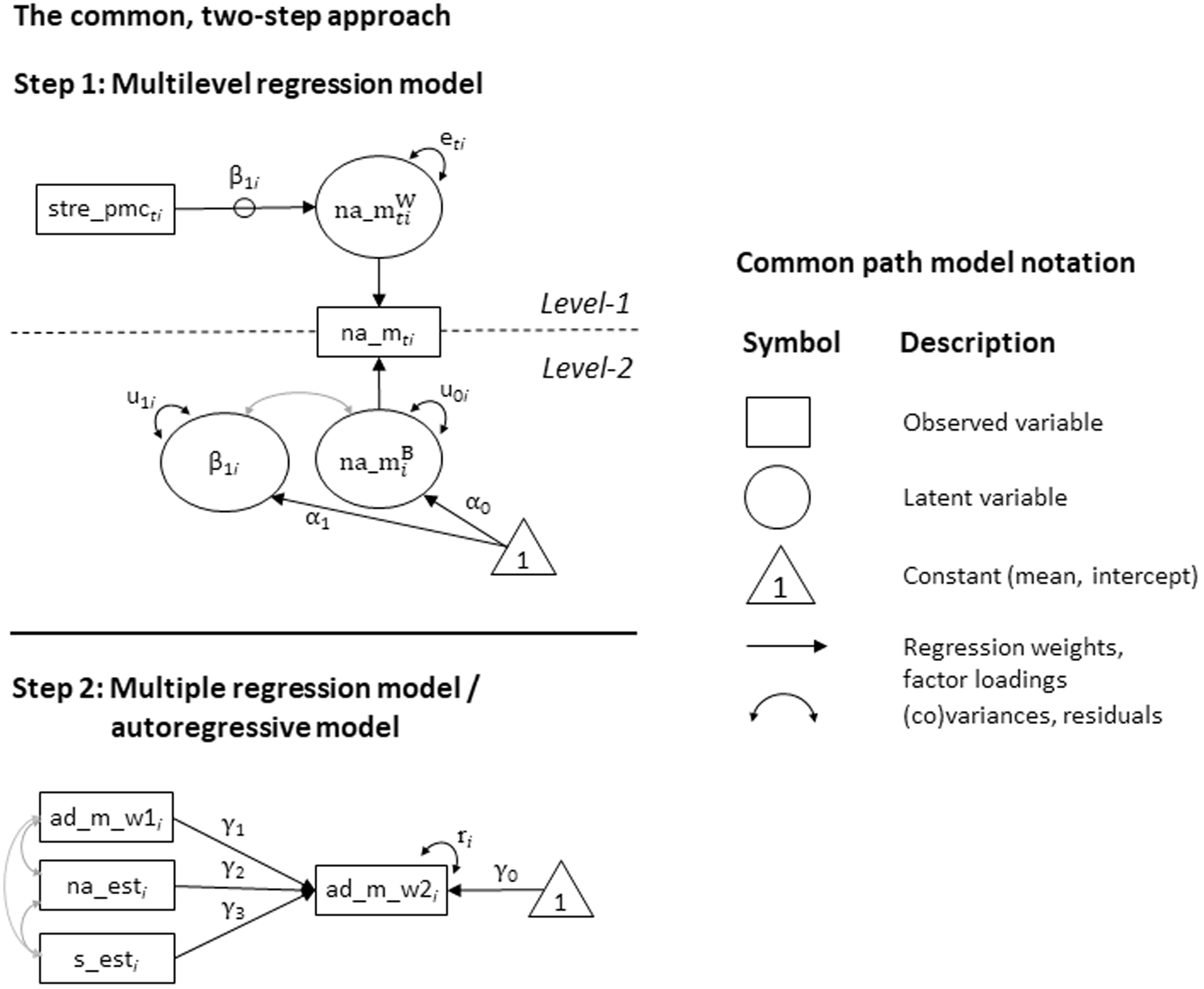
Basic path model diagram of the two-step approach of combining state dynamics (stress reactivity) and trait change (residualized change in affective distress as averaged across three items, ad_m, and across Waves 1/2, w_1/2), including information on common path model notation. Parameters can be mapped onto those of equations (1) and (2); stre = stress, pmc = person-mean centered, na_m = mean negative affect across several items. The Step 1 stress reactivity slope estimates, β_1i, are treated as observed variables (individual slope estimates, s_esti) in Step 2. Grey lines in the figure represent parameters that are estimated but not part of equations (1) and (2).

In Step 1, the observed time-varying variable na_m _ti (in a rectangle), is decomposed into its within (Level 1) and between (Level 2) components, represented by circles at the two levels. The level-1 component, $\text{na}\_{\text{m}}_{ti}^{\text{W}}$ , is regressed on the observed, person-mean centered stressor variable at Level 1, stre_pmc _ti , the predictor and regression effect being indicated by a rectangle and an arrow, respectively, and the latter reflecting stress reactivity. The fixed and random parts of stress reactivity, ${\beta }_{1i}$ , are unobserved level-2 parameters. This is indicated by the black circle on the regression path at Level 1 and the corresponding circle at Level 2. Average stress reactivity ( ${\alpha }_{\text{1}}$ , the fixed effect) is illustrated by a path of the latent variable at Level 2 on a constant (the triangle in Figure 1). Variance in stress reactivity ( ${\text{u}}_{1i}$ , the random effect) is illustrated by the double-headed arrow. The between part of negative affect, $\text{na}\_{\text{m}}_i^{\text{B}}$ , is also graphically represented by a circle at Level 2. Its average ( ${\alpha }_0$ , the fixed effect) is again illustrated by a path on the constant, and the variance in average levels of negative affect ( ${\text{u}}_{0i}$ , the random effect) is illustrated by the double-headed arrow above the circle. Unexplained variance in within-person variation in negative affect, ${\text{e}}_{ti}$ , is represented by the double-headed arrow. Finally, the double-headed arrow between stress reactivity and negative affect at Level 2 illustrates the slope-intercept correlation that is usually estimated in multilevel models including within-person slopes.

Step 2 treats all included variables as if they were directly observed—all variables are represented by rectangles. The observed variable ad_m_w2 _i is regressed on ad_m_w1 _i , the estimates of individuals’ levels of negative affect, na_est _i , and reactivity slope estimates, s_est _i . In addition to the regression paths, ${\text{γ}}_1$ , ${\text{γ}}_2$ , and ${\text{γ}}_3$ , this model estimates the intercept and residual variance of ad_m_w2 _i , ${\text{γ}}_0$ and ${\text{r}}_i$ .

Simulated data on stress reactivity and change in affective distress

We now illustrate this two-step approach further by using simulated data. Using simulated data has the advantage that the true effects are known. This data will also be used for the explanation of all improvements that we suggest in this tutorial. The data is meant to reflect a longitudinal study with 400 participants and two study waves. Wave 1 included a trait assessment and an intensive measurement phase of 100 repeated occasions. In Wave 2, the trait assessment was repeated. The dataset entails information on negative affect and stressor occurrence as observed on each of the 100 occasions. Stress events were coded as 0 and 1 (a stressful event had occurred or not). Negative affect was measured by four items with a continuous answering scale, ranging from −7.5 to 7.5, with higher values indicating higher levels of negative affect. For the analyses, the mean across four items, na_m, was computed for each occasion and individual. Individuals’ trait levels of affective distress were measured using three items and a continuous answering scale, ranging from −5 to 5, with higher values reflecting more affective distress. For the analysis, the mean across the three affective distress items was computed at each wave, ad_m_w1 and ad_m_w2.

The data were simulated on the basis of plausibility considerations: individuals with higher levels of negative affect during the intensive measurement phase were those with a greater proportion of stressor occurrence, higher stress reactivity, and higher levels of affective distress at Wave 1, with correlations ranging from 0.30 to 0.50. There was no average change in affective distress across waves, but individual differences therein. Stress reactivity and mean levels of negative affect across 100 occasions were positively related to increases in affective distress. The exact values used for simulating the data can be found in the simulation script in the accompanying OSF repository, together with the simulated data, input and output files (https://osf.io/3sjr4/).

In addition to analyses using the total sample, we also worked with subsamples to illustrate the effects of sample size (n and t) on results. Subsample 1 consisted of 200 participants with an average of 49.6 occasions (9909 observations, range: 39–61); Subsample 2 consisted of 200 participants with an average of 25 occasions (5012 observations, range: 13–36); and Subsample 3 consisted of 236 participants with 8 occasions (1910 observations, range 5–11).

Results for the common approach using the simulated data

Using this simulated data, we generated the results on the question of whether stress reactivity predicts residualized change in affective distress (set of equations (1) and (2)), using Mplus Code Step 1, 2-step procedure (please see Supplement 1a). Table 1 summarizes the results of Step 1, with a focus on the parameters of major interest: Occasions with stressors were those with enhanced negative affect (i.e. the average within-person stress reactivity slope, ${\alpha }_1$ , differed from zero). The strength of this association varied between individuals, u_1i. The random intercept of negative affect and the random slopes from this MLM (individual estimates of mean negative affect and stress reactivity, respectively) were saved during this step (see Mplus code).

Table 1.

Estimates of the two-step approach and Improvements 1 to 3 using simulated data.

		True est.	Two-step approach		Impr. 1: one-step approach		Impr. 2: latent mean centering		Impr. 3: inclusion measurement models
	Par.		Est.	SE	Est.	SE	Est.	C.I.	Est.	C.I.
N × T = 40,000
Mean stress reactivity	α1	0.30	0.436	0.024	0.437	0.024	0.262	0.235, 0.290	0.308	0.276, 0.343
Variance stress reactivity	u1	0.10	0.202	0.016	0.202	0.016	0.077	0.066, 0.089	0.105	0.090, 0.122
ad_m_w2 / ad_w2 on
ad_m_w1 / ad_w1	γ1	0.40	0.372	0.041	0.366	0.042	0.365	0.283, 0.448	0.413	0.317, 0.511
na_m / na	γ2	0.30	0.270	0.045	0.273	0.046	0.273	0.185, 0.364	0.258	0.166, 0.352
Stress reactivity	γ3	0.90	0.561	0.086	0.561	0.086	0.932	0.662, 1.211	0.856	0.586, 1.112
Subs. 1, N x T = 9909
Mean stress reactivity	α1	0.30	0.430	0.035	0.430	0.035	0.256	0.215, 0.300	0.302	0.254, 0.348
Variance stress reactivity	u1	0.10	0.187	0.024	0.188	0.024	0.072	0.057, 0.092	0.099	0.078, 0.127
ad_m_w2 / ad_w2 on
ad_m_w1 / ad_w1	γ1	0.40	0.401	0.058	0.391	0.059	0.390	0.269, 0.504	0.436	0.302, 0.570
na_m / na	γ2	0.30	0.208	0.059	0.211	0.060	0.204	0.086, 0.327	0.187	0.059, 0.313
Stress reactivity	γ3	0.90	0.623	0.129	0.624	0.130	1.056	0.637, 1.500	0.936	0.539, 1.360
Subs. 2, N × T = 5012
Mean stress reactivity	α1	0.30	0.430	0.039	0.429	0.039	0.245	0.198, 0.292	0.291	0.238, 0.345
variance stress reactivity	u1	0.10	0.192	0.031	0.191	0.031	0.073	0.055, 0.095	0.097	0.073, 0.128
ad_m_w2 / ad_w2 on
ad_m_w1 / ad_w1	γ1	0.40	0.354	0.058	0.343	0.059	0.343	0.221, 0.460	0.374	0.236, 0.507
na_m / na	γ2	0.30	0.386	0.072	0.391	0.074	0.394	0.241, 0.538	0.397	0.218, 0.559
Stress reactivity	γ3	0.90	0.549	0.152	0.545	0.157	0.862	0.336, 1.384	0.864	0.362, 1.354
Subs. 3, N x T = 1910
Mean stress reactivity	α1	0.30	0.446	0.046	0.441	0.046	0.226	0.170, 0.279	0.264	0.202, 0.327
Variance stress reactivity	u1	0.10	0.143	0.043	0.193	0.138	0.064	0.042, 0.094	0.083	0.055, 0.123
ad_m_w2 / ad_w2 on
ad_m_w1 / ad_w1	γ1	0.40	0.428	0.058	0.400	0.047	0.404	0.278, 0.524	0.471	0.318, 0.499
na_m / na	γ2	0.30	0.172	0.070	0.117	0.054	0.209	0.058, 0.357	0.194	0.033, 0.450
Stress reactivity	γ3	0.90	0.675	0.251	0.764	0.321	0.783	0.029, 1.657	0.730	−0.032, 1.586

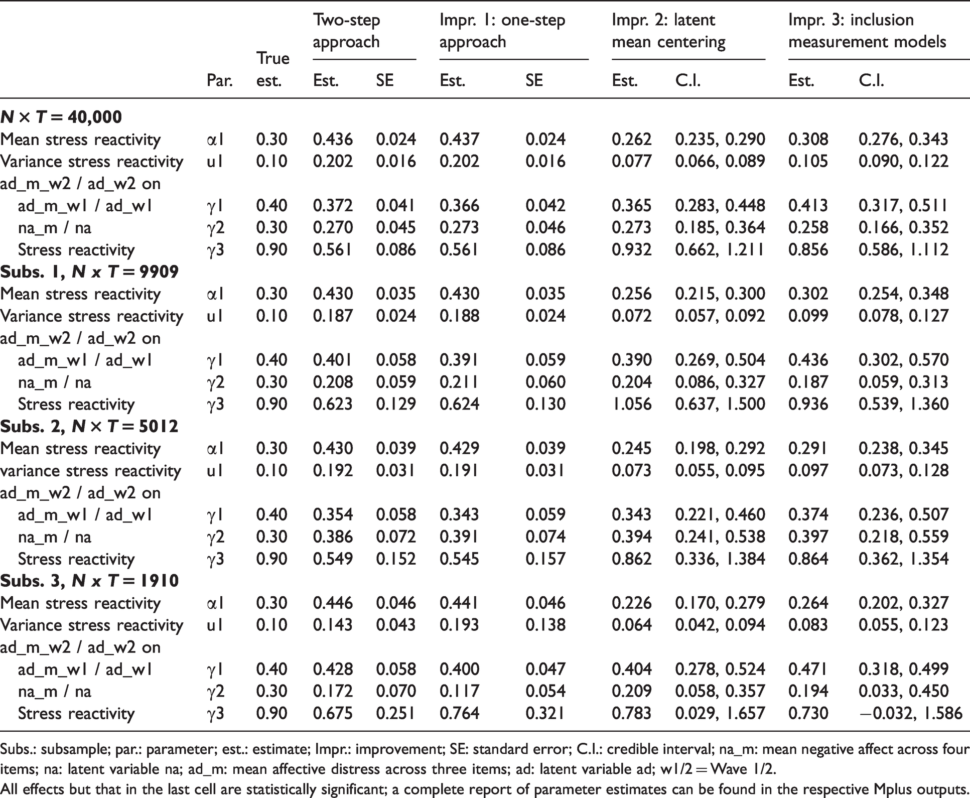
Subs.: subsample; par.: parameter; est.: estimate; Impr.: improvement; SE: standard error; C.I.: credible interval; na_m: mean negative affect across four items; na: latent variable na; ad_m: mean affective distress across three items; ad: latent variable ad; w1/2 = Wave 1/2.

All effects but that in the last cell are statistically significant; a complete report of parameter estimates can be found in the respective Mplus outputs.

We proceeded with Step 2, using Mplus Code for Step 2 (please see Supplement 1b). In this step, the AR model that treated estimates from Step 1 as observed predictors of affective distress, all predictors were significant (Wave 1 affective distress, mean negative affect, and stress reactivity; γ₁ to γ₃). This pattern of findings was also found in the three subsamples. However, according to the increasing standard errors of the estimates, the precision of estimation (and with it also the statistical power) decreased in the subsamples with fewer observations. Nevertheless, if these data had been collected in an empirical study, we would conclude that stress reactivity significantly predicted residualized change in affective distress across waves. Individuals with stronger reactions to stressors were those with higher levels of residualized change, controlling for mean levels of negative affect.

Step-by-step guidance for improved analyses of state variation and trait change

Acknowledging well-established statistical methods and recent developments on state dynamics and trait change, we conceive that three aspects of this two-step approach predicting change in affective distress with reactivity coefficients require being reconsidered: (1) It is a two-step approach with different sources of biases for parameter estimates; (2) it does not correct for sampling error on the side of the predictors; (3) it does not include measurement models and does not provide information on measurement invariance across time. These three aspects can be improved in ML-SEM ³ (Asparouhov et al., 2018; Muthén, 1994). A shift towards these frameworks allows combining modeling state dynamics at Level 1 (e.g. stress reactivity; cf. Rush et al., 2019) with modeling of trait change at Level 2 (e.g. in affective distress or other aspects of well-being).

In a step-by-step fashion, we will now elaborate on each aspect and demonstrate how it can be achieved by using ML-SEM. Key features of each improvement are summarized in Table 2. Although the improvements seem to be a series of increasingly complex ML-SEMs, each model will detail and illustrate a specific possibility for improvement over the two-step approach that stands on its own and can be implemented separately.

Table 2.

Key improvements over the two-step approach as highlighted in this tutorial, and information on data and software requirements.

	Two-step approach	Improvement 1: one-step approach	Improvement 2: latent mean centering	Improvement 3: inclusion of measurement models
Key advantage(s) over common Two-step approach		• Correct estimation of SEs of effect of random slopes	• Correct estimation of latent mean of level-1 predictor variable (i.e. level-2 covariate)• Centering of level-1 predictor around individuals’ latent means	• Examination of relations at construct level• Consideration of item-specific item-factor associations• Possibility to examine measurement invariance
Requirements of data per step	• Step 1: multiple occasions• Step 2: at least two waves	• Same as for common approach	• Same as for common approach	• Multiple indicators per construct• Else: same as for common approach
Statistical procedures	• Step 1: MLM• Step 2: multiple regression	• ML-SEM	• ML-SEM	• ML-SEM
Estimation procedure	• ML, OLS regression, or Bayesian	• Maximum likelihood or Bayesian	• Bayesian	• Maximum likelihood or Bayesian
Software	• Step 1: any MLM software• Step 2: any basic statistics software	• Mplus	• Mplus, Version 8.3 and later	• Mplus

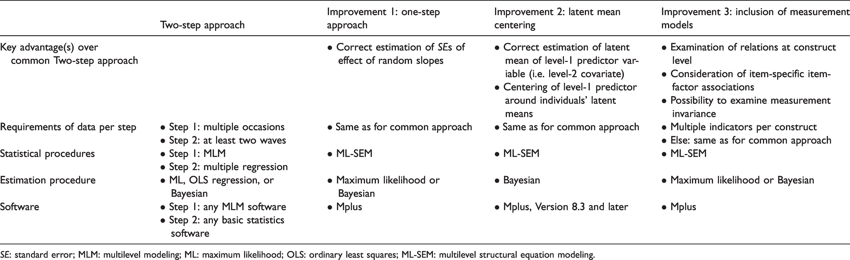
SE: standard error; MLM: multilevel modeling; ML: maximum likelihood; OLS: ordinary least squares; ML-SEM: multilevel structural equation modeling.

Improvement 1: Overcoming the two-step approach

Problem: Biased standard error estimates in two-step procedures

A disadvantage of the two-step approach is that the individual slope estimates from Step 1 (i.e. the stress reactivity estimates) are treated as observed variables in Step 2, not as estimated values. This, in turn, results in an underestimation of the standard error of the effect of stress reactivity on affective distress in Step 2, and thus, in potentially excessively-liberal significance testing at this Step 2 (Frischkorn et al., 2016; Skrondal & Laake, 2001). Underestimation of the standard error in Step 2 is related to the reliability of the individual slope estimates reflecting stress reactivity. This reliability depends on various factors (e.g. the number of measurement occasions in the case of intensive longitudinal data, level-1 predictor variance; Liu et al., 2019; Neubauer et al., 2020; Raudenbush & Bryk, 2002). It may thus vary across studies with different numbers of occasions, but also across individuals of the same study. When using individual slope estimates in the second step of the two-step approach (i.e. when treating them as observed scores), information on their reliability is not considered in the prediction of some outcome variable—one treats them as if reliability was perfect.

Together, when treating slope estimates as observed predictors, one runs the risk of claiming a statistically significant effect of the slope estimate (i.e. ${\text{γ}}_3$ ), even if the true effect is zero, more often than the nominal alpha error rate (inflated Type-I error). Apparently, this provides a major threat for replicability and cumulative knowledge gain in psychological research.

Solution

These problems can be overcome by switching to a one-step approach using ML-SEM (e.g. Rush et al., 2019). Like MLM, ML-SEM is suited for working with nested data. Additionally, ML-SEM allows specifying multiple outcome variables and paths among them simultaneously—this happens in the structural parts of the models. Using ML-SEM thus allows a flexible combination of the parameters of the two-step approach: While modeling stress reactivity at Level 1, the between-person component of negative affect and the reactivity slope, as well as change in affective distress across waves, can all be modeled simultaneously. Most importantly, the effect of reactivity on change in affective distress, formerly tested in Step 2, can be modeled as one among other relations at Level 2 in ML-SEM. Put differently, the reactivity slope can become a predictor in ML-SEM, specifically a predictor of affective distress in our example. The disadvantages of the two-step approach alluded to above (reliability of person-specific estimates; attenuated standard errors obtained in two-step approaches) are overcome this way.

Formal representation

The formal representation of the first improvement that turns the two-step into a one-step approach and integrates the analysis of state dynamics and trait change is highly similar to that of equations (1a) to (1d) and (2). The only, but essential, aspect that changes is that the prediction of change in affective distress by stress reactivity is now part of the model (i.e. it is no longer handled in a separate multiple regression analysis)

$$\text{na}\_{\text{m}}_{ti}=\text{na}\_{\text{m}}_{ti}^{\text{W}}+\text{na}\_{\text{m}}_i^{\text{B}}$$

(3a)

$$\text{Level }1\text{na}\_{\text{m}}_{ti}^{\text{W}}={\beta }_1{\hspace{0.17em}}_i{\text{ stre\_pmc}}_{ti}+{\text{e}}_{ti}$$

(3b)

$$\text{Level}2\text{na}\_{\text{m}}_i^{\text{B}}={\alpha }_0+{\text{u}}_{0i}$$

(3c)

$${\beta }_{1i}={\alpha }_1+{\text{u}}_{1i}$$

(3d)

$$\text{ad}\_\text{m}\_\text{w}{2}_i={\text{γ}}_0+{\text{γ}}_1\text{ad}\_\text{m}\_\text{w}{1}_i+{\text{γ}}_2\text{na}\_{\text{m}}_i^{\text{B}}+{\text{γ}}_3{\beta }_{1i}+{\text{r}}_i$$

(3e)

Up to the third row, the model is equivalent to that represented by equations (1a) to (1d). What is new is the last row (equation (3e)). It relates the modeling of state dynamics to the modeling of trait change. Here, affective distress at Wave 2, ad_m_w2 _i , is a function of an intercept, ${\text{γ}}_0$ , affective distress at Wave 1, ad_m_w1 _i , individuals’ average levels of negative affect as simultaneously estimated in this model, $\text{na}\_{\text{m}}_i^{\text{B}}$ (equation (3c)), and, importantly, the individual slopes reflecting stress reactivity, ${\beta }_{1i}$ , also estimated in this model (equation (3d)). Equation (3e) is similar to equation (2), but only when integrating this equation with the preceding can the level-2 estimates of individuals’ mean negative affect and stress reactivity be simultaneously used as predictors of affective distress at Wave 2—these estimates are both outcome and predictor variables.

Path diagram, Mplus code, and results

The path diagram representing equations (3a) to (3e) illustrates the integration of Steps 1 and 2 of the two-step approach (Figure 2(a)).

Figure 2.

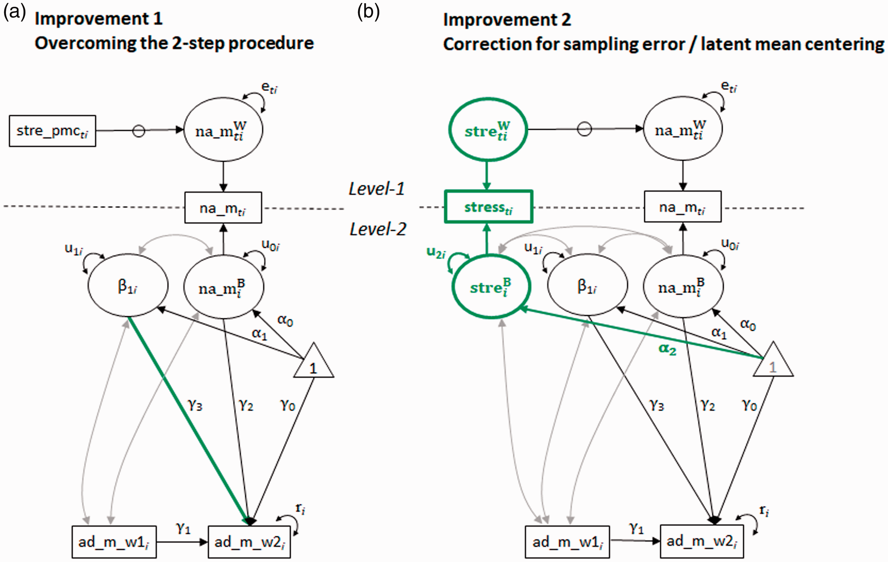
(a) Integration of the analysis of state dynamics and trait change; (b) correction for sampling error and latent mean centering; stre = stress, pmc = person-mean centered, na_m = mean negative affect across four items, ad_m_w1/2 = mean affective distress across three items at Wave1/2. The aspect of either approach that is advantageous in comparison to the two-step approach is highlighted in green; parameters can be mapped onto those of equations (3) and (4). Grey lines in the figure represent parameters that are estimated but not part of equations (3) and (4).

The stress reactivity slope including its fixed and random part at Level 2, ${\beta }_{1i}$ , now predicts affective distress at Wave 2, as indicated by the path ${\text{γ}}_3$ . Similarly, affective distress is predicted by the between-person component of negative affect, $\text{na}\_{\text{m}}_i^{\text{B}}$ , as indicated by the path ${\text{γ}}_2$ . The simultaneity of estimation in this approach with flexible modeling of structural paths among variables thus is also obvious in its graphical representation. The other illustrated parameters are comparable to those described in the context of Figure 1. Not reflected by the equations, but estimated and drawn in this figure, are also the correlations between all level-2 exogenous variables (stress reactivity, negative affect, and affective distress at Wave 1).

The Mplus code of this model as realized as a ML-SEM is provided in Supplement 2, Mplus Code I, Improvement 1. The results from this model can also be found in Table 1. In the complete sample, the estimates are very similar to those of the two-step approach. Focusing on the effect of central interest and the complete sample, the average stress reactivity slope as well as individual differences therein are statistically significant, and stress reactivity predicted residualized change in affective distress at Wave 2, ${\text{γ}}_3$ . The standard error of ${\text{γ}}_3$ was indistinguishable across approaches in the complete sample. The advantage of the one-step over the two-step approach—the potential underestimation of the standard error when treating individual estimates from MLM as observed—thus did not become obvious here. Yet, turning to the subsamples with fewer observations reveals that this specific standard error increased from the two-step to the one-step approach, especially when the number observations decreases: Compared to the standard error from the two-step approach, the standard error from the one-step approach increased by 0.8% in Subsample 1 (200 participants, on average 50 observations per participant), by 3.3% in Subsample 2 (200 participants, on average 25 observations per participant), and by 28% in Subsample 3 (236 participants, on average eight observations per participant). This clearly hints at the problem of the two-step approach that is addressed with Improvement 1: a potential underestimation of the standard error (in particular when the number of repeated observations per participant decreases) which might, in turn, result in erroneous conclusions on the prospective effects of stress reactivity.

Improvement 2: Correction for sampling error, latent mean centering

Problem: Sampling error

Another aspect of the two-step approach that is not yet ideal is that it does not correct for sampling error at the side of predictors. Sampling error may bias estimates if individuals contribute limited amounts of information in, for example, experience sampling studies in which individuals answer prompts on fewer than the planned number of occasions. The problem of sampling error at the side of predictors was brought up in the context of contextual variables (Lüdkte et al., 2008). Contextual variables are level-2 aggregates of variables that are measured at Level 1 and aggregated per level-2 unit. They can be used to predict level-2 components of some outcome variable. In the case of our example, stressors could be aggregated into person-specific proportions of stressor occasions across the sampling period. This level-2 aggregate would then be referred to as a contextual variable that could be used to predict levels of negative affect at Level 2 in the multilevel model. If one computes level-2 aggregates; however, a problem emerges: the aggregates are only approximations of the unobserved “true” scores (Lüdtke et al., 2008) because in the case of varying numbers of sampled occasions per level-2 unit (i.e. a different number of occasions per individual), the reliability of aggregated level-2 covariates may vary across level-2 units: The average number of occasions with a stressor can be estimated with higher reliability for those participants with more occasions.

In our specific case, we are not interested in the effects of the level-2 component of stressors per se, but it is relevant for centering stressor occurrence: Stressor occurrence has been person-mean centered in this tutorial thus far, and stressors were centered around computed, person-specific proportions of stressor occasions. Relating this back to the elaborations of the preceding paragraph, one thus only works with approximations, but not true scores of these proportions of stressor days, when centering the stressor variable. Given that the reliability of these approximations may vary across participants, this might have subsequent effects on the person-mean centered level-1 predictor variable.

Solution

These problems can be addressed by applying the latent covariate approach (Lüdtke et al., 2008) and by latent mean centering (Asparouhov & Muthén, 2018). In the latent covariate approach, the unobserved true means of level-1 variables (proportions of stressor days in our example) are estimated and treated as latent variables (Lüdtke et al., 2008). That is, just as negative affect, the outcome variable in the multilevel part of our models, stressors as level-1 predictors can be decomposed into their latent level-1 and a level-2 component. This amendment corrects for unreliability of level-2 covariates due to sampling and “results in unbiased estimates of L[evel-]2 constructs” (Lüdtke et al., 2008, p. 203). Of note is that one needs to use the Bayesian estimator in Mplus in order to take full advantage of latent mean centering for dichotomous predictors (Mplus 8.3 or later).

Once having switched to this latent covariate approach, one can also use latent mean centering instead of centering predictors manually by subtracting computed averages. In latent mean centering, the estimated latent level-2 component of a predictor is used to center level-1 components of predictors. This procedure was recently extended to also accommodate categorical predictors (Asparouhov & Muthén, 2018). It prevents working with only approximations of person means of within-person predictors, and should, in turn, result in less biased estimates of person-specific slope estimates (person-specific stress reactivity slopes in our example). Together, latent mean centering implies superior centering of level-1 predictors because the latter are centered around their latent means.

Formal representation

When applying the latent covariate approach and latent mean centering, the equations of our model on stress reactivity and change in affective distress are as follows

$$\text{na}\_{\text{m}}_{ti}=\text{na}\_{\text{m}}_{ti}^{\text{W}}+\text{na}\_{\text{m}}_i^{\text{B}}$$

(4a)

$${\text{stress}}_{ti}={\text{stre}}_{ti}^{\text{W}}+{\text{stre}}_i^{\text{B}}$$

(4b)

$$\text{Level }1\text{ na}\_{\text{m}}_{ti}^{\text{W}}={\beta }_{1i}{\text{stre}}_{ti}^{\text{W}}+{\text{e}}_{ti}$$

(4c)

$$\text{Level }2\text{ na}\_{\text{m}}_i^{\text{B}}={\alpha }_0+{\text{u}}_{0i}$$

(4d)

$${\beta }_{1i}={\alpha }_1+{\text{u}}_{1i}$$

(4e)

$${\text{stre}}_i^{\text{B}}={\alpha }_2+{\text{u}}_{2i}$$

(4f)

$$\text{ad}\_\text{m}\_\text{w}{2}_i={\text{γ}}_0+{\text{γ}}_1\text{ad}\_\text{m}\_{\text{w}}_{1i}+{\text{γ}}_2\text{na}\_{\text{m}}_i^{\text{B}}+{\text{γ}}_3{\beta }_{1i}+{\text{r}}_i$$

(4g)

Now both time series, negative affect and stressor occurrence, ${\text{na}}_{ti}$ , and stressor _ti , are decomposed into within- and between-person variance components. Modeling the two stressor components means to apply the latent covariate approach. The two components reflect that stressor occurrence varies within individuals across occasions and that the proportion of stressor occasions varies across persons. The between component of stressors is now modeled at Level 2, ${\text{stre}}_i^{\text{B}}$ , which should result in bias-free estimates of individuals’ proportion of stressors occasions (equation (4f)). ${\text{Stre}}_i^{\text{B}}$ is a function of the threshold ⁴ for stressor occurrence, ${\alpha }_2$ , as well as individual differences therein, ${\text{u}}_{2i}$ . Important in view of stress reactivity predicting affective distress, this estimated level-2 stressor component is used for centering the within-person component of stressors, ${\text{stre}}_{ti}^{\text{W}}$ .

Path diagram, Mplus code, and results

Figure 2(b) represents the model just described.

The observed stressor variable (rectangle) is now decomposed into its two level-specific components (represented by circles), similar to the decomposition of negative affect. The threshold for stressor occurrence at Level 2 is represented by its regression on the constant, ${\alpha }_2$ , and variance in this threshold is indicated by the double-headed arrow on the level-2 component of stressors, ${\text{u}}_{2i}$ . The Mplus code for this model is provided in Supplement 3, Mplus Code II, Improvement 2. The results (Table 1) reveal some deviation of the point estimates in comparison to the preceding models. The within-person stress reactivity slope (fixed and random effect, ${\alpha }_1{\text{ and u}}_{1i}$ , became smaller and closer to the true parameter estimates that are known in simulated data. In the total sample, the estimate for stress reactivity predicting residualized change in affective distress came closer to the true effect (0.933 vs. 0.561, respectively, the true value being 0.9). This pattern was similar when using only subsets of the simulated data for analyses.

As briefly mentioned above, latent mean centering of predictors requires the Bayesian estimator in Mplus. Consequently, the estimates’ statistical significance in this model is no longer based on the estimates’ standard errors and confidence intervals, but on credible intervals. Also, we examined the convergence of this model using Bayesian estimation by visual inspection of the trace plots of posterior parameter estimates, and by inspection of maximum probability of scale reduction. Below, we provide recommendations on how to familiarize with these aspects of Bayesian estimation.

Improvement 3: Inclusion of measurement models

Problem 3: Measurement error

Up to now, the analyses did not take full advantage of the data regarding the constructs’ measurement with multiple items: four negative affect items, and three affective distress items at each wave. We thus far used averages across items (na_m, ad_m_w1, ad_m_w2), which comes with several disadvantages: measurement error is not corrected for and heterogeneous item-construct relations are not considered. To illustrate, one assumes that all indicators of negative affect such as hostile, nervous, and jittery reflect a construct equally well—although one may suspect that hostile is not that closely related to a construct that is otherwise measured by nervous and jittery (cf. Brose et al., 2020). Finally, measurement invariance across multiple measurement occasions cannot be tested without measurement models.

Solution

The solution to these problems is well known: measuring constructs with multiple indicator variables (e.g. items) and employing latent variable models—an essential part of SEM, and realizable in ML-SEM. The latent variables resulting from the inclusion of measurement models are free of measurement error and allow for heterogeneous item-construct relations by freely estimating the factor loadings. The latent factors thereby capture only the variance that is common to the set of indicator variables and allow for testing relations among variables at the construct level. Using latent variable models in longitudinal research also allows testing for measurement invariance across occasions. Establishing measurement invariance is necessary to be sure that one has measured the same construct across occasions (Meredith, 1994). Assuming some basic knowledge on latent variable modeling/confirmatory factor analysis, we keep background information short. Moreover, the integration of latent variable models and multilevel models is not new (Marsh et al., 2009; Muthén, 1994). Nevertheless, we are not aware of a study on state dynamics and change in well-being that applied latent variable modeling and thus introduce it as an additional advantage.

Formal representation

Measurement models in SEM are commonly represented by equations such as

$${\text{x}}_k={\alpha }_k+{\lambda }_k\eta +{\text{ζ}}_k$$

(5)

Here, a latent variable, $\text{η}$ (for example negative affect), is measured with multiple indicator variables, x _k , with indicators 1 to j (e.g. nervous, hostile). The observed indicator variables are a function of the latent variable $\text{η}$ , multiplied by item-specific loadings ( ${\lambda }_k$ , regression weights relating the latent with the observed variables), item-specific intercepts, ${\alpha }_k$ , and item-specific residuals, ${\text{ζ}}_k$ . For a set of items 1 to j, the matrix notation of the resulting system of equations is

$$\text{X}=\alpha +\Lambda \eta +\text{ζ}$$

(6)

Here, X is a vector of j observed variables (e.g. nervous, hostile), $\text{α}$ and Λ are vectors of j intercepts and loadings, the latter being multiplied by the latent variable η, and a vector of j residuals, $\mathrm{\zeta }$ . Such measurement models can also be specified for multilevel data. Remember the variance decomposition of na_m (the mean across the four negative affect items) as was done in equation (1a). Just as this variable was shown to have a within- and between-person variance component, vectors of multiple observed variables measuring latent constructs can be decomposed. Assume the latent variable negative affect, na (without _m), was measured with four items within individuals across occasions. Variance decomposition now pertains to all four observed na items, ${\text{na}}_k$ , k = 1, … , 4.

$$\text{na}{k}_{ti}=\text{na}{k}_{ti}^{\text{W}}+\text{na}{k}_i^{\text{B}}$$

(7a)

Based on this decomposition, measurement models can be set up at both levels of analysis, resulting in the following set of equations

$${\text{stress}}_{ti}={\text{stre}}_{ti}^{\text{W}}+{\text{stre}}_i^{\text{B}}$$

(7b)

$$\text{Level }1\text{ na}{k}_{ti}^{\text{W}}={\lambda }_{\text{na}k}^{\text{W}}{\text{na}}_{ti}^{\text{W}}+{\text{e}}_{k,ti}$$

(7c)

$${\text{na}}_{ti}^{\text{W}}={\beta }_{1i}{\text{stre}}_{ti}^{\text{W}}+{\text{e}}_{ti}$$

(7d)

$$\text{Level }2\text{ na}{k}_i^{\text{B}}={\alpha }_{3k}+{\lambda }_{\text{na}k}^{\text{B}}{\text{na}}_i^{\text{B}}+{\text{u}}_{3k,i}$$

(7e)

$${\text{na}}_i^{\text{B}}={\alpha }_0+{\text{u}}_{0i}$$

(7f)

$${\beta }_{1i}={\alpha }_1+{\text{u}}_{1i}$$

(7h)

$${\text{stre}}_i^{\text{B}}=a_2+{\text{u}}_{2i}$$

(7g)

$$\text{ad}\_\text{w}1k_i={\alpha }_{4k}+{\lambda }_{\text{ad}\_\text{w}1k}^{\hspace{0.17em}}\text{ad}\_\text{w}{1}_i+{\text{u}}_{4k,i}$$

(7i)

$$\text{ad}\_w2k_i={\alpha }_{5k}+{\lambda }_{\text{ad}\_\text{w}2k}^{\hspace{0.17em}}\text{ ad}\_\text{w}{2}_i+{\text{u}}_{5k,i}$$

(7j)

$$\text{ad}\_\text{w}{2}_i={\text{ γ}}_0+{\text{γ}}_1\text{ad}\_\text{w}{1}_i+{\text{γ}}_2{\text{na}}_i^{\text{B}}+{\text{γ}}_3{\beta }_{1i}+{\text{r}}_i$$

(7k)

Level 1 now specifies a measurement model for the latent variable negative affect, na. The within-person component of each item, $\text{na}{k}_{ti}^{\text{W}}$ , with k = 1, … , 4, is a function of the product of the within-person loadings, ${\lambda }_{\text{na}k}^{\text{W}}$ , and the within-person latent variable negative affect, ${\text{na}}_{ti}^{\text{W}}$ , which varies across occasions and individuals. The residual of this equation, ${\text{e}}_{k,ti}$ , denotes variance in the na indicators that is unexplained by the latent variable. The latent variable ${\text{na}}_{ti}^{\text{W}}$ is then predicted by stressor occurrence in the next equation (7d). At Level 2, the measurement model for the latent variable na is similar to the one at Level 1, but it is based on the between-person variance components of the observed variables, $\text{na}{k}_i^{\text{B}}$ , and it includes a vector of intercepts, ${\text{α}}_{3k}$ . The latent na variable at Level 2, ${\text{na}}_i^{\text{B}},$ is modeled to have a mean ( ${\alpha }_0$ ) and variance ( ${\text{u}}_{0i}$ ). In addition, the equations at Level 2 now include measurement models for affective distress at Waves 1 and 2. These measurement models include intercepts, product terms (loadings multiplied by the latent affective distress variables), and item-specific residual terms. The prediction of the latent variable affective distress at Wave 2, $\text{ad}\_{\text{w2}}_i$ , is now based on the latent variables, $\text{ad}\_{\text{w1}}_i$ , ${\text{na}}_i^{\text{B}}$ , and stress reactivity, ${\beta }_{1i}$ . Together, the model represented by equations (7a) to (7k) includes measurement models and thus corrects for measurement error, and potentially unequal item-construct relations are considered.

Path diagram, Mplus code, and results

Figure 3 represents this model and may look complicated at first sight. Yet, it is similar to Figure 2(b), with the difference that it entails measurement models for the latent variables negative affect and affective distress. All indicator variables are represented by rectangles, and these are regressed on their specific factors, the loadings represented by arrows and indicating their regression weights, ${\lambda }_{\text{na}k}^{\text{W}}$ , ${\lambda }_{\text{na}k}^{\text{B}}$ , ${\lambda }_{\text{ad}\_\text{w}1k}^{\hspace{0.17em}}$ , and ${\lambda }_{\text{ad}\_\text{w}2k}^{\hspace{0.17em}}$ . Residual variances of the indicator variables as well as of the emerging latent variables are represented by double-headed arrows. The structural paths of this model are now exclusively among constructs: the latent variable negative affect, ${\text{na}}_{ti}^{\text{W}}$ , is regressed on stressors at the within-person level, and the latent variable affective distress at Wave 2, $\text{ad}\_{\text{w2}}_i$ , is regressed on affective distress at Wave 1, the latent variable negative affect at Level 2, and the between components of stress reactivity. Additionally, the figure represents correlations among level-2 variables that are estimated but not part of equations (7a) to (7k).

Figure 3.

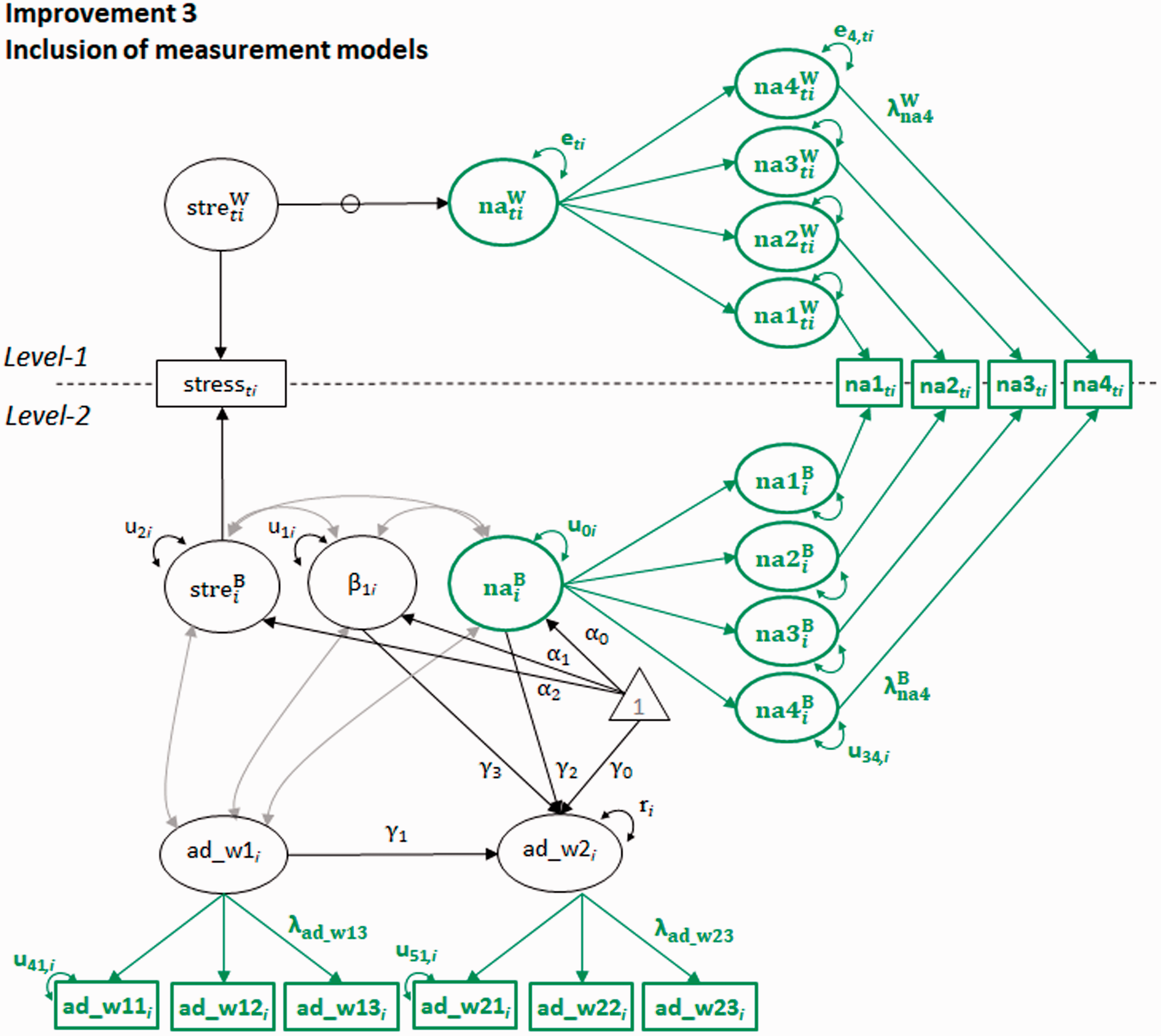
Correction for measurement error by including measurement models; stre = stress, na = negative affect, ad = affective distress, _w1/2 = Wave1/2. The aspect that is advantageous in comparison to the two-step approach and to the one preceding in the model series is highlighted in green; parameters can be mapped onto those of equations (7). Grey lines in the figure represent parameters that are estimated but not part of equations (7). To reduce complexity, some parameters are not depicted: intercepts of na and ad indicators, loadings 2 and 3 of na, loadings 2 of ad at Waves 1 and 2.

We ran this model using the Bayesian estimator to also keep Improvement 2; it could also have been run using maximum likelihood estimation when using a computed person-mean centered stress variable instead. The Mplus code for this model is provided in Supplement 4, Mplus Code III, Improvement 3. Prior to the estimation of the model just described, we tested whether the same latent variable affective distress was measured at the two waves (i.e. we tested for measurement invariance). This was done by specifying measurement models for affective distress and by constraining multiple parameters of the wave-specific measurement models to equality (i.e. the loadings, intercepts, and variances of the indicator variables; see Mplus files “sim_data_measurement_invariance” for details). Model fit indices indicated strict measurement invariance, χ² [14] = 12.554, p = 0.561; RMSEA = 0.00, CFI = 1.00, SRMR = 0.022. Thus, the latent variable was measured across waves in a comparable way. Moreover, the loadings indicate heterogeneity of item-construct relations.

The results of Improvement 3 are reported in Table 1. These show that the true parameters were recovered well (the 95% credible interval contains the true parameters) and point estimates were generally closer to the true parameters than those of the two-step procedure and Improvement 1. This holds for the entire sample and the subsamples. Note, however, that the effect of the reactivity slope on affective distress was not significant in Subsample 3 according to the credible interval, likely hinting at the imprecision of estimation with small samples. In some cases, the point estimates of Improvement 2 were closer to the true parameters than those of Improvement 3, but these differences were small.

Intermediate summary

Based on all results generated with the simulated data, one would conclude that state dynamics and trait change are related (as just noted, with the exception of Subsample 3, Improvement 3): Stress reactivity predicted residualized change affective distress at Wave 2. While the parameter estimates of the prospective effect of stress reactivity were identical in the two- and one-step approach (Improvement 1), they were closer to the true estimates in Improvements 2 and 3. Given this pattern of results, conclusions would not differ between the approaches if we only took a dichotomous (significant vs. not significant) criterion to evaluate the effects. However, the effect of stress reactivity on residualized change in affective distress might be underestimated when not considering sampling error and measurement error. Moreover, the difference between the one- and two-step approach became clearer when using a subsample of observations for analysis (Subsample 3). Here, the standard error of estimation for the effect of stress reactivity on affective distress increased in the one-step approach. Given prior work on this issue (Skrondal & Laake, 2001), the larger standard error in the one-step approach should be less biased than the smaller one in the two-step approach, hinting at the danger of excessively liberal significance testing in Step 2 of the latter. Together, this pattern of findings implies that a suboptimal modeling strategy can potentially lead to either false-positive or false-negative results, or to an under- or overestimation of point estimates.

Empirical example

To illustrate further how to integrate the analysis of state dynamics and trait change, and how changes in the analytical approach may change the results, we reanalyzed data from the National Study of Daily Experiences (NSDE) as used by Charles et al. (2013; for details on the data, see Supplement 7). The results of the two-step approach, including the same set of predictors as were used by Charles et al. and pursuing the similar procedures, conceptually replicated those reported in the original publication ⁵ (Supplement 7; for syntax of all models, see folder NSDE on OSF): Stress reactivity predicted residualized change in affective distress over 10 years; more stress reactivity predicted higher affective distress.

We proceeded with a model series using the same data-analytical premises as for the simulated data. That is, other than Charles et al. (2013), we worked with a person-mean centered stressor variable and included mean levels of negative affect as predictors of residualized change in affective distress. For simplicity, we dropped age, education, and gender from the analyses. We then ran the same model series on the NSDE data (N = 832, T = 5943) as for the simulated data: Step 1 and 2 of the two-step approach, followed by Improvements 1 to 3, and switching to Bayesian estimation when running Improvements 2 and 3.

Results are presented in Table 3. Starting with Step 1 of the two-step approach: Negative affect was enhanced on stressor occasions, α1 = 0.076, and individuals differed in the strength of this within-person effect, u1 = 0.012. In Step 2, when individuals’ stress reactivity estimates were used for the prediction of affective distress at Wave 2 in the AR model, in addition to mean negative affect and affective distress at Wave1, stress reactivity did not predict residualized change in affective distress above and beyond the other predictors, γ3. When switching to the one-step approach (Improvement 1), small deviations in the parameter estimates occurred, but the pattern of results remained comparable. In line with the articulated problem of the two-step approach, there was a slight increase in the standard error of the effect of stress reactivity on affective distress at Wave 2 (1.34% increase, while the regression effect slightly decreased from −0.010 to −0.008). This seems to hint at the problem of too liberal significance testing in the two-step approach. When implementing Improvement 2, latent mean centering, the point estimates of negative affect (γ2) and stress reactivity (γ3) on affective distress at Wave 2 diverged from the preceding models. Taking the significance criterion for comparing the different approaches, one would still come to the same conclusions across models (only negative affect is a significant predictor of affective distress, not stress reactivity). Yet, if one was interested in the estimates’ size, interpretations would diverge. When attempting to include measurement models (Improvement 3), while keeping Improvement 2, we encountered estimation problems according to the potential scale reduction value (1.033) and according to the trace plots of several parameter estimates (please see Mplus outputs), even after having increased the number of iterations when estimating the models. We thus fitted Improvement 3 using maximum likelihood estimation and without applying latent mean centering. Again, some differences in the estimates emerged. Specifically, the point estimate of the effect of stress reactivity on residualized change in affective distress, γ3, became more negative, but it remained non-significant.

Table 3.

Estimates of the common approach and Improvements 1 to 3 using the empirical example.

		Two-step approach		Impr. 1: one-step approach		Impr. 2: latent mean centering		Impr. 3: inclusion measurement models
	Par.	Est.	SE	Est.	SE	Est.	C.I.	Est.	SE
N = 832, T = 5943
Mean stress reactivity	α1	0.076	0.007	0.076	0.007	0.044	0.034, 0.054	0.070	0.009
Variance stress reactivity	u1	0.012	0.002	0.012	0.002	0.015	0.013, 0.017	0.021	0.003
ad_m_w2 / ad_w2 on
ad_m_w1 / ad_w1	γ1	0.353	0.033	0.322	0.037	0.316	0.224, 0.387	0.362	0.050
na_m / na	γ2	0.882	0.228	0.941	0.224	1.116	0.776, 1.473	0.815	0.281
Stress reactivity	γ3	−0.010	0.446	−0.008	0.452	−0.075	−0.479, 0.318	−0.243	0.396

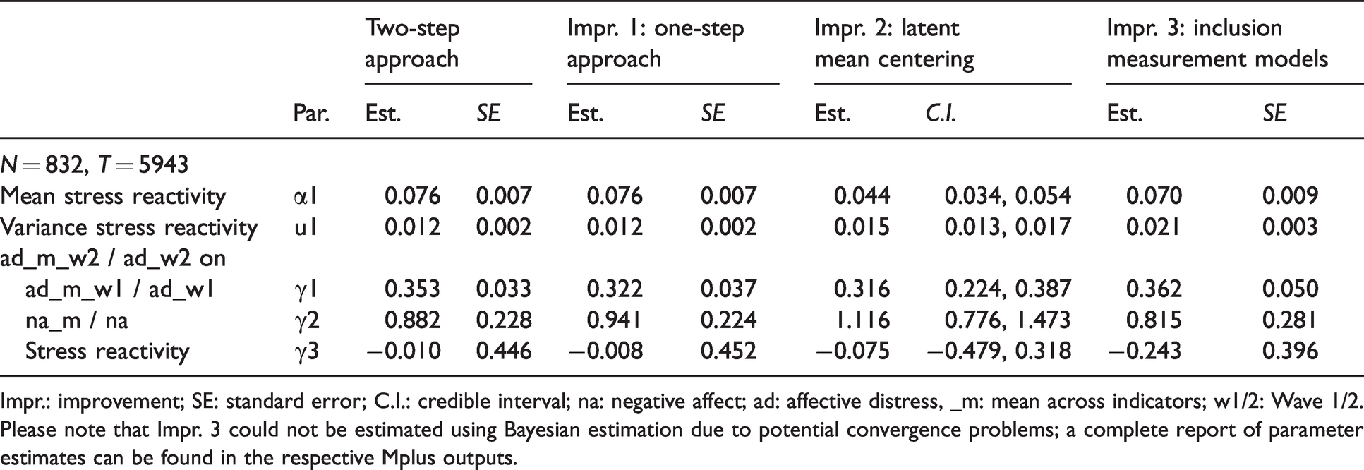
Impr.: improvement; SE: standard error; C.I.: credible interval; na: negative affect; ad: affective distress, _m: mean across indicators; w1/2: Wave 1/2.

Please note that Impr. 3 could not be estimated using Bayesian estimation due to potential convergence problems; a complete report of parameter estimates can be found in the respective Mplus outputs.

In summary, when using empirical data and implementing the modeling improvements as detailed above, the results also revealed variations in parameter estimates. These were expected in case of the decreased standard error of the effect of stress reactivity on affective distress at Wave 2. Regarding the other parameters, their true values are not known. Still, it was obvious that the size of the point estimates in Improvement 2 and 3 changed to a considerable degree. In this model series, stress reactivity did not predict residualized change in affective distress. This divergence from the original result (Charles et al., 2013 and our conceptual replication) might be attributable to centering the stressor variable or to including mean negative affect in the analyses, instead of the variable “negative affect on non-stressor days”. We get back to the role of the mean in these and related analyses below.

Practical recommendations and notes on modeling decisions

Having detailed specific aspects that can be improved when integrating state dynamics and trait change, and having demonstrated changes in parameter estimates related to the improvements, we now turn to some more general practical recommendations and notes on modeling decisions. We first allude to more general advantages of ML-SEM over 2-step approaches, proceed with highlighting advantages of turning to Bayesian estimation, and then elaborate on sample size.

General advantages of ML-SEM over two-step approaches

Another reason to switch to a one-step approach using ML-SEM is that it is the more parsimonious data-analytical approach. Also, the practical handling of data is less prone to errors (e.g. because one does not need to merge estimates from Step 1 with another data set for Step 2), and one can work with the missing-at-random assumption in SEM (if one assumes, for example, that individuals’ missing data is related to other study variables such as stress levels). This should produce less biased estimates on the basis of all available data, which is superior to listwise deletion as is common in the two-step approach.

Bayesian estimation

The improvements that were explained in this tutorial were realized with two different estimation procedures, maximum likelihood estimation and Bayesian estimation in Mplus (i.e. latent mean centering of predictor variables as explained in the context of Improvement 2 requires the latter). Although the use of Bayesian methods has reached psychological science, so far it does not seem to be routine applied by researchers. This might impede adequate specifications that are needed for model estimation as well as the evaluation of information provided together with results (e.g. evaluation of trace plots that are provided for each parameter estimate and that hint at estimation problems). To familiarize the reader with these aspects, we can highly recommend the materials provided on the Mplus website (https://www.statmodel.com/). Another potentially problematic aspect with using the Bayesian estimator is that one probably encounters convergence problems more often than when using maximum likelihood estimation. These might be facilitated, however, by adjusting the parameter priors (from the default flat priors to weekly informative priors; Lemoine et al., 2019).

Besides, we see clear advantages of using the Bayesian estimator: First, it allows to estimate models that are substantially more complex than what would be possible in a maximum likelihood framework (e.g. random effects of all level-1 parameters, including residual variances and covariances; see Hamaker et al., 2018). This flexibility of Bayesian estimation makes this approach a very powerful tool to approach the complex interplay among a multitude of variables. Second, Bayesian estimation in Mplus provides standardized effects (not available with ML estimation), which is relevant, for example, when one would be interested in comparing the predictive value of various state dynamics on trait change (e.g. of affective reactivity and affect’s residual variance). Third, the Bayesian estimator in Mplus is implemented such that it can deal with unequally spaced measurement occasions. Specifically, observations can be structured in accordance with a superimposed time grid with equal spacings (e.g. days in a diary study; the choice of time grids shall be close to the empirical spacings). In case of distances between observations that are longer than the time grid spacing, time points that are not used are substituted by missing values. This way, the emerging time series becomes approximately equidistant (Hamaker et al., 2018; cf. McNeish & Hamaker, 2019, for a good explanation of this issue). This is an advantage when working with intensive longitudinal data in which samplings are either (quasi-) random by design, as is often the case in experience sampling studies, or when persons miss out on answering questionnaires at random—the resulting unequally spaced time series are often ignored in MLM, with unknown effects on parameter estimates.

Sample size

A one-step approach is generally preferable to a two-step approach as argued above (deflated standard error). However, a one-step approach might require larger level-2 sample sizes. Simulation work targeting ML-SEM for mediation models shows that with small samples (e.g. 60–100 participants at Level 2 or less) ML-SEM might yield less favorable statistical properties than multilevel models (e.g. McNeish, 2017). Hence, with a relatively small number of participants, ML-SEM should be used with caution. We note, however, that in cases with only a small number of participants, statistical power in a two-step approach will also be limited. Therefore, when the aim is to predict between-person change in traits from within-person dynamics, a reasonably large level-2 sample size (>100) is likely called for, and in these settings, the one-step approach via ML-SEM might be expected to outperform the two-step approach.

The number of repeated observations per participant affects the precision of the person-specific estimates of within-person dynamics (Neubauer et al., 2020). Hence, a too low number of repeated assessments reduces the relative amount of true between-person variability in the slopes, and, in turn, decreases statistical power to detect potential effects of the slope estimates on trait change (see, e.g. the nonsignificant effect of the reactivity slope on affective distress in Improvement 3, Subsample 3). The number of repeated observations required to obtain a requested level of reliability can be estimated if reasonable model parameters can be estimated a priori (see Neubauer et al., 2020).

The advantage of using latent mean centering over centering on the manifest person mean (Improvement 2) should attenuate when the number of repeated assessments increases: With many repeated observations per participant, an individual’s person mean can be estimate with high reliability and, hence, the difference between the estimated person mean and the latent person mean will become smaller. However, in cases of unbalanced designs (i.e. participants differ in the number of data points they provide), there will be heterogeneity in the reliability of the person means that is not accounted for when using manifest person-mean centering.

Taken together, both the sample size on Level 2 (the number of participants) and Level 1 (the number of repeated assessments per participant) play a vital role in models predicting long-term trait change from within-person dynamics. Adequate and reliable estimates via the often superior one-step approach likely require sample sizes of 100 participants or more. When using latent variables (see Improvement 3) minimal sample size requirements increase further. Future research using comprehensive simulation work is, however, required to determine the relative advantage of one-step versus two-step approaches for various sample sizes on Level 1 and Level 2.

Inclusion of the mean

In our brief review of studies examining prospective effects of stress reactivity on change in well-being, average levels of negative affect were not always included in the prediction of change in well-being. However, the mean of dynamically varying variables, specifically affective experiences, were recently shown to be an essential aspect when predicting trait measures (Dejonckheere et al., 2019). In fact, Dejonckheere et al. revealed that predicting well-being outcomes from dynamic aspects of time series data is often close to negligible once the mean level of the dynamically varying variable is controlled for. In turn, not including means when examining state dynamics might lead to inflated estimates of the predictive utility of the latter for long-term outcomes (see also Dejonckheere et al., 2019). We therefore included mean levels of negative affect into our analyses. From a theoretical point of view, however, a specific state dynamic might be more relevant for trait change than its related mean levels. For example, recovery from a negative event might be particularly difficult if one endures comparatively strong affective reactions when reminded of the event. Even though such comparatively strong reactions should also be reflected in mean levels of affect, it might be more relevant from a treatment perspective to identify the potential cause behind mean levels (e.g. stress reactivity; Neubauer et al., 2021)—a treatment could then focus on how to attenuate strong affective reactions.

Together, the statistical dependence of state dynamics and corresponding mean levels need to be kept in mind when relating state dynamics and trait change. Yet, whether and how this dependence is dealt with and which aspect is prioritized in prediction is also a matter of theoretical considerations.

Outlook on alternative applications

In this tutorial, we focused on a specific type of state dynamics (stress reactivity), one type of trait change (residualized change across two waves approached with an AR model), and we examined one specific direction of effects—the prospective effects of reactivity on trait change. This specification is but one from a whole range of applications within the general modeling framework that we elaborated upon. That is, the statistical tools we explained provide much flexibility to answer a multitude of questions. As we will now exemplify, modifications are possible such that one can examine (1) other state dynamics, (2) other types of trait change, or (3) other directions of effects. Mplus codes for these alternative applications are provided in the folder Outlook_alternative_models on OSF, https://osf.io/3sjr4/.

State dynamics beyond stress reactivity

One may be interested in whether state dynamics other than stress reactivity predict changes in well-being, for example affect variability or the persistence of affect across time (i.e. its lagged effect; cf. Dejonckheere et al., 2019, for a summary of different indicators of state dynamics). Estimating various state dynamics including time-lagged effects simultaneously can be realized by working in the dynamic structural equation modeling (DSEM) framework ⁶ in Mplus (Asparouhov et al., 2018). This furthermore allows the simultaneous prediction of some outcome variable with these various state dynamics, as was recently demonstrated by Hamaker et al. (2018). More specifically, these authors explained how to model two related time series using a bivariate vector autoregressive model. The parameters that were simultaneously modeled were the means across occasions (i.e. of positive and negative affect), the variables’ lagged effects, their cross-lagged effects, their residual variances as well as the residuals’ covariance. Still in the same step, all these state dynamics were used to predict (Level 2) depressive symptoms.

Schematic figure and Mplus code

A schematic figure of this model, highlighting its state dynamics, is provided in Figure 4(a). For the reader who is interested in its estimation, we refer to the Mplus codes provided by Hamaker et al. (2018). These codes can also be used to integrate the respective state dynamics with residualized change in some outcome variable.

Figure 4.

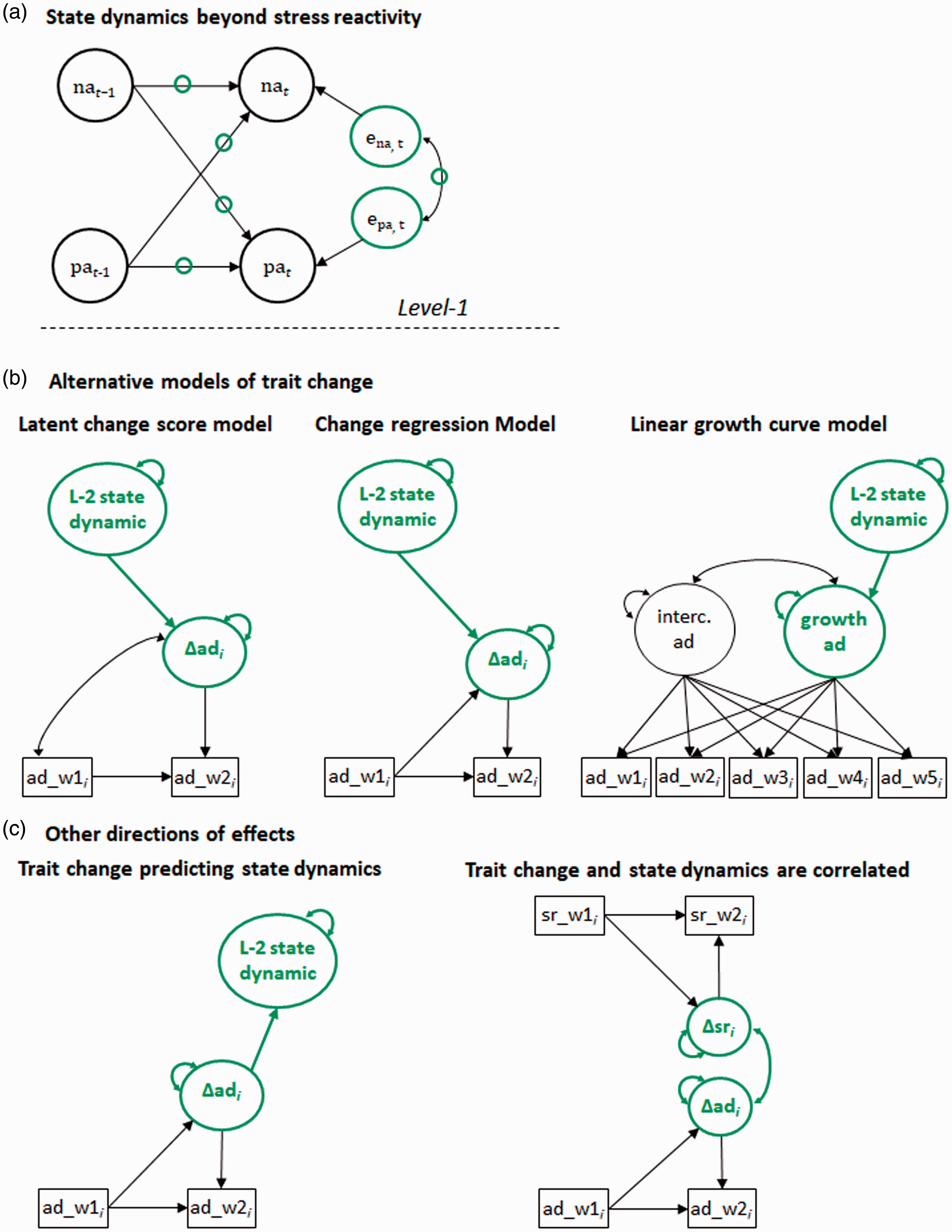
(a) Schematic figures of level-1 state dynamics beyond stress reactivity; (b) alternative models of trait change; (c) other directions of effects; na = negative affect, pa = positive affect, ad = affective distress, w1/2 = Wave1/2, sr = stress reactivity. In (a), the green circles represent different aspects of state dynamics as emerging in a bivariate vector autoregressive model that can be integrated with trait change: lagged effects and residual variances of na and pa, cross-lagged effects among pa and na, the covariance among the pa–na residuals. In (b), the latent change score (left) and change regression model (middle) capture change across two waves via latent variables; the growth factor (right) captures change across five occasions; in turn, latent change or growth, are integrated with state dynamics in (b). In (c), left side, trait change as modeled with the change regression model predicts future state dynamics. In (c), right side, trait change and change in state dynamics are correlated.

Alternative models of trait change

To broaden the scope of this tutorial, we highlight two types of trait change in the following that are modeled commonly and that can be integrated with state dynamics: change across two waves approached with change score models and linear growth across multiple waves. Regarding the latter, one could speculate whether the pace of recovery of well-being after the experience of some critical life event (i.e. individual differences in longitudinal growth) is prospectively predicted by how strongly individuals react to daily stressors (cf. Zhaoyang et al., 2020, for a related example).

Change across two waves approached with latent change models

Instead of linking state dynamics with trait change across two occasions by means of the AR model, as we did in this tutorial, one can establish links with absolute change. To do so, one could use the latent change score model (LCSM; e.g. McArdle & Nesselroade, 1994). The LCSM is a SEM that has been developed for two-wave data. Essential to the LCSM is the estimation of a latent change factor which is characterized by two parameters, a mean and a variance term, reflecting average change and individual differences therein (for a recent tutorial on the LCSM, see Kievit et al., 2018). Taking the example of two-wave data on affective distress, a latent change score model provides information on whether persons’ levels of affective distress change across waves on average, and whether individuals differ therein. Importantly, and similar to the one-step procedures in Improvements 1 to 3, once the LCSM is established, one can relate the latent change variable with other variables of a ML-SEM, such as stress reactivity—the latent change variable can be treated as one among multiple variables of the structural part of a (ML-)SEM.

Of note, the AR model of this tutorial can also be specified as a change model. This is achieved by regressing latent change in affective distress on affective distress at Wave 1. The emerging change regression model is entirely equivalent to the AR model—the parameters of these modes are reparameterizations of each other (see, e.g. Castro-Schily & Grimm, 2018). The difference between the LCSM and the AR or change regression model, however, is far from trivial, and practical recommendations on when to use which model diverge (cf. Lüdtke & Robitzsch, 2020, for a recent review and comparison of both models). At the conceptual level, the models differ regarding the research questions that they answer: the LCSM examines whether change (e.g. in affective distress) is associated with some treatment effect (e.g. stress reactivity); the AR model examines whether a treatment (e.g. stress reactivity) predicts subsequent affective distress, conditioning on prior affective distress.

Schematic figures and Mplus codes

Figure 4(b), left side, is a schematic of the LCSM in which the latent change score is predicted by some state dynamic. Most importantly for the integration of state dynamics and trait change, the latent change variable, for example reflecting change in affective distress, includes a variance term (the double-headed arrow). This variance in change can be linked to state dynamics (e.g. stress reactivity), by regression paths. Thus, this model again reflects a combined analysis of state dynamics and trait change. Figure 4(b), middle, is a schematic of the change regression model. The small but impactful difference between Figure 4(b), left and middle, is the regression path from affective distress at Wave 1 to the latent change factor. In the latter, change is adjusted for individual differences in affective distress at Wave 1. The Mplus codes for the LCSM and the change regression model are very similar; please see input file “Outlook_LCSM_and_change_regression_model” on OSF.

Linear change across multiple waves using growth curve models

In studies with several assessment waves, the models of change can be constructed as latent growth curve model (LGCMs; e.g. McArdle, 2009) or as neighboring change models (see Quintus et al., 2020). For example, maturation of personality or stability and decline of well-being can be approached with such models. In essence, LGCMs model within-person change by regressing some outcome variable such as affective distress on time (e.g. waves). Growth is unobserved and modeled by one (or multiple, in case of polynomial change) growth factor(s). Growth factors have an intercept, indicating mean change across time, and a variance component, indicating individual differences therein. If approached in the ML-SEM framework, this variance component can be integrated with state dynamics–the growth factor can be predicted or can predict state dynamics such as stress reactivity. Again, the growth factor then is one of multiple variables of the structural part of a ML-SEM. To our knowledge, only one study thus far has used a statistical approach as promoted in this paper to link state dynamics with longitudinal growth (Zhaoyang et al., 2019, linked stress reactivity to change in depressive symptoms using ML-SEM).

Schematic figure and Mplus code

Figure 4(b), right side, is a schematic of a linear LGCM. Observations across time are modeled as indicators of both a latent intercept and a growth factor. The latent growth factor has a variance term, indicating individual differences in change. The latter are integrated with state dynamics, by the regression path on some state dynamic. The model’s Mplus code, using the example of stress reactivity predicting linear change in affective distress, is referred to as “Outlook_growth_model” on OSF.

Other directions of effects

State dynamics may not only precede trait change. Instead, trait change may also precede (changes in) state dynamics. For example, facing prolonged illness may decrease trait resilience, which, in turn, may enhance stress reactivity. In this case, the strength of stress reactivity would be the consequence of trait change. Taking this one step further, state dynamics and trait change may exert reciprocal effects on each other (cf. Roberts, 2018). For example, unexpected job loss may result in both, increases in stress reactivity and increases in trait level affective distress, and these increases may be correlated across time.

Schematic figures and Mplus codes

When conceptualizing state dynamics as the outcome of trait change, one needs to model trait change explicitly as done in the LCSM or the change regression model. This way, the respective state dynamic can be regressed on the change factor. Figure 4(c), left side, is a schematic of this idea, to be realized with the Mplus code “State_dynamic_as_outcome_of_change”. The correlated change model is represented by Figure 4c, right side. Here, one models latent change of some trait and latent change of stress reactivity and lets these two factors correlate. An important requirement for using this model is a correct structuring of the data; a schematic of a correctly structured data set is provided along with the Mplus code for this model, “Correlated_change” on OSF.

Together, predicting trait change from stress reactivity is but one of a whole world of modeling possibilities when interested in the integration of state dynamics and trait change. In this world, one can simultaneously examine various indicators of state dynamics, model different types of change, and the direction of effects can be conceptualized differently. This last section shall have paved the path for transferring the general improvements alluded to alternative research questions.

Caveats and limitations

The present tutorial style paper aimed to illustrate the advantages of three improvements compared to the two-step approach to predict trait change from state dynamics. To that end, we used a simulated data set with a fixed set of true population parameters and demonstrated that all three improvements aid in recovering the true parameters. A limitation of the model series presented in Tables 1 and 3 is that improvements across models can only roughly be quantified. Switching between modeling frameworks (MLM, ML-SEM) and estimation procedures (maximum likelihood and Bayesian estimation) as well as comparing non-nested models prevents the use of test statistics to compare models. Nevertheless, our simulated example aimed to raise awareness that simple models may yield suboptimal (and potentially even wrong) conclusions if the true model is more complex than the model used. Moreover, we made certain assumptions about the “true” model that may or may not represent the true associations of these constructs in empirical work. To that end, these findings merely illustrate that if these assumptions (including an effect of stress reactivity on trait change, normally and independently distributed residuals, …) hold in reality, the model incorporating all three improvements is able to recover them well. The extent to which parameters can be recovered if these assumptions do not hold (e.g. when there are autoregressive residuals, or when there is no effect of reactivity on trait change) was not determined in the present work. Moreover, how the models perform under varying design characteristics (e.g. number of participants, number of repeated observations per participant, mechanisms of missing data, deviations from normal distribution, …) require extensive simulations studies that were outside the scope of the present work.

Conclusion

In a paper on state-of-the-art methods of modeling state dynamics and future challenges in this field of research, it was noted that “how to relate moment-to-moment and day-to-day processes to developmental processes spanning years or even a lifetime, is one of the fundamental questions that will be begging an answer over the following decade” (Hamaker et al., 2015, p. 321). With recent methodological advancements, large steps were made to meet these challenges (e.g. Asparouhov et al., 2018), and researchers have started using these advancements (e.g. Hertzog et al., 2017; Zhaoyang et al., 2019). We add to this field of research a tutorial paper in which we, with substantive researchers in mind, promote and explain in detail how to simultaneously model state dynamics and trait change using the example of stress reactivity and change in affective distress. We used ML-SEM as implemented in Mplus and elaborated on three improvements when relating state dynamics and trait change with the currently available modeling techniques. Using simulated data, we showed that parameter estimates became closer to the true parameter estimates when incorporating the improvements. This pattern was corroborated when using real data (Charles et al., 2013). Hence, methodological variations may affect the results, and the two-step modeling approach to the integration of state dynamics and trait change needs to be reconsidered. We hope to have convinced the readers that switching to more advanced methods is feasible with the available software, and indeed has advantages over the two-step approach. As an outlook, we sketched how these improvements may also find further applications.

Supplemental Material

sj-pdf-1-erp-10.1177_08902070211014055 - Supplemental material for Integrating state dynamics and trait change: A tutorial using the example of stress reactivity and change in well-being

Supplemental material, sj-pdf-1-erp-10.1177_08902070211014055 for Integrating state dynamics and trait change: A tutorial using the example of stress reactivity and change in well-being by Annette Brose, Andreas Benjamin Neubauer and Florian Schmiedek in European Journal of Personality