Sage Journals: Discover world-class research

Abstract

French

Correspondence analysis (CA) is a popular technique to visualize the relationship between two categorical variables. CA uses the data from a two-way contingency table and is affected by the presence of outliers. The supplementary points method is a popular method to handle outliers. Its disadvantage is that the information from entire rows or columns is removed. However, outliers can be caused by cells only. In this paper, a reconstitution algorithm is introduced to cope with such cells. This algorithm can reduce the contribution of cells in CA instead of deleting entire rows or columns. Thus the remaining information in the row and column involved can be used in the analysis. The reconstitution algorithm is compared with two alternative methods for handling outliers, the supplementary points method and MacroPCA. It is shown that the proposed strategy works well.

Keywords

contingency table incidence matrix MacroPCA outliers supplementary points visualization

Introduction

Correspondence analysis (CA) is an exploratory data analysis method which visualizes the dependence of the two categorical variables in a two-way contingency table using a two-dimensional plot (Gower & Hand, 1996; Greenacre, 1984, 2017, 2018; Greenacre & Hastie, 1987). CA has received considerable attention in a variety of areas such as education (Kienstra & Van der Heijden, 2015), marketing (Pitt et al., 2020), psychology (Kim et al., 2021), and text categorization and authorship attribution (Qi et al., 2024). However, relatively little attention has been given to CA in the presence of outliers (Riani et al., 2022).

Outliers may be errors or unexpected observations which could shed new light on the researched phenomenon (Sripriya & Srinivasan, 2018). In general data structures, not contingency tables, the data are arranged in a matrix where rows correspond to the individual observations and columns are variables (Grubbs, 1969; Hubert et al., 2019; Raymaekers & Rousseeuw, 2024; Rousseeuw & Van Den Bossche, 2018). The term outlier typically refers to an individual observation that deviates markedly from other members of the sample in which it occurs (Andersen & Mayerl, 2017; Robette, 2022).

However, in a contingency table, the definition of an outlier is different (Kuhnt et al., 2014; Sripriya & Srinivasan, 2018). An entry in the table represents the number of individuals that occurs jointly in a category of one variable and a category of the other. Thus, in the contingency table, a row does not correspond to a single observation but to a number of joint sample frequencies of individual observations. Here, extreme counts that do not follow the general pattern in the table are viewed as outliers.

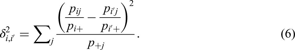
In the context of CA, an outlier can be defined in different ways and the procedure to detect outliers depends on the definition of an outlier. Two detection procedures stand out. On the one hand, Greenacre (2013, 2017) uses visual inspecting of CA plots to detect outliers. Greenacre (2013, 2017) considers a row or column point as an outlier when it clearly lies far from other points in the CA plot. In addition to large absolute coordinates, Hoffman and Franke (1986) and Bendixen (1996) define a row or column point as an outlier if the row or column point has a high contribution to an axis. The contribution of a point to an axis is determined not only by the position of the point in the CA plot but also by the marginal proportion of the point. According to Hoffman and Franke (1986) and Bendixen (1996), if the marginal proportion of a point is very small, it may not be an outlier, even though, following Greenacre’s definition, it is an outlier in the sense that it lies far from other points in the CA plot.

On the other hand, Riani et al. (2022) and Raymaekers and Rousseeuw (2024) detect outliers making use of distributional assumptions. Riani et al. (2022: 8) state “an outlier is a row which does not agree with the multiplicative model assuming independence fitted to the data.” This outlier detection procedure is less attractive, because, in interesting applications, the independence model assumption would be rejected almost always (De Leeuw et al., 1990), and thus, in this situation, this procedure tends to detect too many rows as outlying points. Raymaekers and Rousseeuw (2024) use MacroPCA to detect outliers. MacroPCA is originally proposed by Rousseeuw and Van Den Bossche (2018) for principal component analysis (PCA) and subsequently used in CA by Raymaekers and Rousseeuw (2024). MacroPCA assumes that the data are generated from a multivariate Gaussian distribution. However, the two variables in the contingency table are categorical variables, and therefore the normality assumption for the input matrix of MacroPCA may be not appropriate for CA.

Hoffman and Franke (1986), Bendixen (1996), Greenacre (2017) and Riani et al. (2022) detect outlying rows or columns, and, after detecting the outliers, they cope with the outliers by the supplementary points method. That is, CA is performed on the contingency table without the outlying rows and columns. Afterwards, the outliers are projected into the CA solution of the reduced table. Therefore, the outliers cannot determine the CA solution.

In contrast, Raymaekers and Rousseeuw (2024) detect outlying cells and outlying rows and handle the outliers in the same step. The basic idea is to impute the outlying cells by an iterative PCA algorithm while excluding outlying rows. Their method does not have a good fit with the theory of CA, and important properties of CA, such as that Euclidean distances in a CA display can be interpreted as approximations of chi-squared distances between rows and between columns of contingency table, are lost. Moreover, this method seems to flag a lot more rows as outliers than necessary.

The supplementary points method and MacroPCA delete outlying rows or columns completely, and therefore, also remove information from these rows or columns that is not related to this outlying problem. So, the removal of an entire row or column causes a unnecessary loss of information.

According to Bendixen (1996), a cell frequency that causes its row to be identified as an outlier might also cause its column to be identified as an outlier, and vice versa. Thus, an outlying row or column may be caused by a specific joint frequency. This suggests that we only need to deal with the specific cell and do not need to delete the entire row or column.

In this paper, the focus is on cell-wise outliers. To detect outlying cells, we follow Greenacre’s definition and use visual inspection of the CA plot. This is because (1) a main aim of CA is to summarize the structure of data via a two-dimensional plot; (2) such outliers cause the other points to be tightly clustered; (3) thus such outliers reduce the readability of a CA plot. A cell is an outlying cell if the corresponding row and column points of this cell lie far from other points. Here, once a cell is identified as an outlier, the cell is not removed but its contribution is reduced. For reducing the contribution of an outlying cell, the reconstitution algorithm is proposed. The reconstitution algorithm has been proposed originally by Nora-Chouteau (1974) and has later been used by Greenacre (1984) and De Leeuw and Van der Heijden (1988) to handle missing values in cells.

The paper is built up as follows. We start with a description of CA background. The next section “Methods to handle outliers” presents the reconstitution algorithm to handle cell-wise outliers and describes MacroPCA and the supplementary points method. Section “Experimental Studies” compares these three methods in simulated data. The next empirical section compares these three methods on a contingency table, the brands of cars dataset, and compares the reconstitution algorithm and the supplementary points method on an incidence table, the ocean plastic dataset. Finally, we discuss and conclude this paper; the last section introduces the implementation of code.

Correspondence analysis background

Let X be a contingency table having I rows and J columns with non-negative entries $x_{i j}$ , and suppose that X has full rank. An index is replaced by ‘+’ when summed over the corresponding elements, such as $x_{i +} = \sum_{j} x_{i j}$ . It is customary to rescale X to the correspondence matrix $P = X / x_{+ +}$ , so that $\sum_{i} \sum_{j} p_{i j} = 1$ . The row profile for row i is the vector with elements $p_{i j} / p_{i +}, j = 1, \dots, J$ and, similarly, the column profile for column j is the vector with elements $p_{i j} / p_{+ j}, i = 1, \dots, I$ . The average row profile is the vector with elements $p_{+ j}, j = 1, \dots, J$ , i.e., the column margins, and the average column profile is the vector with elements $p_{i +}, i = 1, \dots, I$ , i.e. row margins. Let $E = [p_{i +} p_{+ j}]$ be the matrix with elements under statistical independence. Let $D_{r}$ and $D_{c}$ be diagonal matrices with the row margins $p_{i +}$ and column margins $p_{+ j}$ in the diagonal, respectively.

CA can be introduced in many ways. We introduce CA here using the concept of total inertia (Greenacre, 2017), i.e., the well-known Pearson $χ^{2}$ statistic divided by $x_{+ +}$ :

Total inertia = \sum_{i} \sum_{j} \frac{{(p_{i j} - p_{i +} p_{+ j})}^{2}}{p_{i +} p_{+ j}} .

(1)

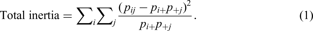
The aim of CA is to provide a multidimensional representation of the matrix X where the total inertia is projected as much as possible onto a low-dimensional space. The computational procedure to obtain the solution makes use of the singular value decomposition (SVD). In the first step the matrix X is transformed into the matrix of standardized residuals $D_{r}^{- 1 / 2} (P - E) D_{c}^{- 1 / 2}$ with elements $(p_{i j} - p_{i +} p_{+ j}) / \sqrt{p_{i +} p_{+ j}}$ , and then SVD is applied to this matrix, yielding

D_{r}^{- 1 / 2} (P - E) D_{c}^{- 1 / 2} = U Σ V^{T},

(2)

where $U^{T} U = V^{T} V = I$ and $Σ$ is a diagonal matrix with singular values $σ_{k}, k = 1, \dots, \min (I - 1, J - 1)$ in descending order on the diagonal. The rank of $D_{r}^{- 1 / 2} (P - E) D_{c}^{- 1 / 2}$ is one less than that of P, because the matrix E of rank 1 is subtracted from P.

If we pre-multiply and post-multiply both sides of Equation (2) by $D_{r}^{- 1 / 2}$ and $D_{c}^{- 1 / 2}$ , respectively, on the left hand side we get $D_{r}^{- 1} (P - E) D_{c}^{- 1}$ with elements $(p_{i j} - p_{i +} p_{+ j}) / (p_{i +} p_{+ j})$ , and this yields

D_{r}^{- 1} (P - E) D_{c}^{- 1} = D_{r}^{- 1 / 2} U Σ (D_{c}^{- 1 / 2} V)^{T} = Φ Σ Γ^{T} = F Σ^{- 1} G^{T}

(3)

where

Φ = D_{r}^{- 1 / 2} U

Γ = D_{c}^{- 1 / 2} V

F = Φ Σ

, and

G = Γ Σ

Φ

and

Γ

are called the standard coordinates for the row profiles and column profiles, respectively. They have the property that, for each k, their weighted sum is 0 and their weighted sum of squares is 1, i.e.

1^{T} D_{r} Φ = 1^{T} D_{c} Γ = 0^{T}

(4)

and

Φ^{T} D_{r} Φ = Γ^{T} D_{c} Γ = I .

(5)

F

and G are called principal coordinates for the row profiles and column profiles, respectively.

Euclidean distances between rows of F ( $G$ ) are equal to the so-called $χ^{2} -$ distances between rows (columns) of X. The squared $χ^{2} -$ distance between the row profiles i and $i^{'}$ is

δ_{i, i^{'}}^{2} = \sum_{j} \frac{{(\frac{p_{i j}}{p_{i +}} - \frac{p_{i^{'} j}}{p_{i^{'} +}})}^{2}}{p_{+ j}} .

(6)

The $χ^{2} -$ distance $δ_{i, i^{'}}$ between row profiles i and $i^{'}$ gives more weight to differences in a column j when this column has a lower margin $p_{+ j}$ . The $χ^{2} -$ distance $δ_{j, j^{'}}$ between column profiles j and $j^{'}$ is defined in a similar way.

Joint graphic displays of row points and column points are usually made to study the relationship between the rows and the columns in the matrix P. For this asymmetric and symmetric maps are used. In an asymmetric map rows of P can be displayed as points in a multidimensional space using principle coordinates, and columns as points using standard coordinates. Thus, in full-dimensional space the dot products of row points F and column points $Γ$ are equal to the elements of $D_{r}^{- 1} (P - E) D_{c}^{- 1}$ . Usually low-dimensional representations are made of the first few columns of F and $Γ$ , as the SVD ensures that the first few dimensions provide an optimal approximation of $D_{r}^{- 1 / 2} (P - E) D_{c}^{- 1 / 2}$ in a least-squares sense. Together, the configurations of row points and column points form a biplot (Gabriel, 1971) of the matrix $D_{r}^{- 1} (P - E) D_{c}^{- 1}$ . Asymmetric maps have the interesting property that the row points are in the weighted average of the column points and the other way around. This is evident from the so-called transition equations

F = D_{r}^{- 1} P Γ and G = D_{c}^{- 1} P^{T} Φ .

(7)

The points for the average row profile and the average column profile fall in the origin. Thus, for the combination of F and $Γ$ , the transition formulas pull individual row points towards the column points for which $p_{i j} / p_{i +} > p_{+ j}$ .

Asymmetric maps have drawbacks. For example, when the pair F and $Γ$ is used, the Euclidean distances between the columns are not chi-squared distances. Also, there is the practical disadvantage that the cloud of column points may be huge in comparison to the cloud of row points, and thus row points tend to huddle together which reduces the readability of the plot. For this reason one often sees the use of the so-called symmetric map. That is, both rows and columns are displayed in principle coordinates. Therefore, the Euclidean distances between row points, i.e., rows of F (column points, i.e., rows of $G$ ) are equal to the $χ^{2} -$ distances between rows (columns) of X, and in low-dimensional representations the Euclidean distances between row points and between column points provide approximations of these chi-squared distances of X. The Euclidean distance between row points F and column points G is not meaningful. However, the direction between row points F and column points G is still meaningful, because the only difference between principal and standard coordinates is a dimensionwise scalar (compare Equation (3)).

The total inertia can be expressed as a weighted sum of squared $χ^{2} -$ distances of row profiles and of column profiles to the average profile:

Total inertia = \sum_{i} p_{i +} \sum_{j} \frac{{(\frac{p_{i j}}{p_{i +}} - p_{+ j})}^{2}}{p_{+ j}} = \sum_{j} p_{+ j} \sum_{i} \frac{{(\frac{p_{i j}}{p_{+ j}} - p_{i +})}^{2}}{p_{i +}} .

(8)

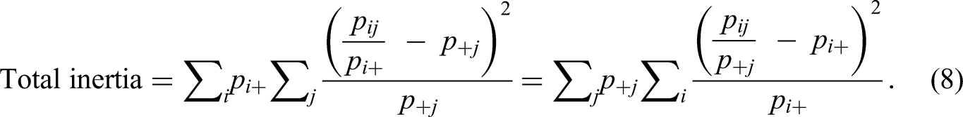
This shows that the total inertia can be split up over the rows and over the columns. The inertia of the row point i and the column point j in dimension k are $p_{i +} f_{i k}^{2} = u_{i k}^{2} σ_{k}^{2}$ and $p_{+ j} g_{j k}^{2} = v_{j k}^{2} σ_{k}^{2}$ , respectively. The contributions of row i and column j to dimension k are $p_{i +} f_{i k}^{2} / σ_{k}^{2} = u_{i k}^{2} σ_{k}^{2} / σ_{k}^{2} = u_{i k}^{2}$ and $p_{+ j} g_{j k}^{2} / σ_{k}^{2} = (v_{j k} σ_{k})^{2} / σ_{k}^{2} = v_{j k}^{2}$ , respectively. The contributions quantify to what extent individual rows and columns, both by their positions ( $f_{i k}$ or $g_{j k}$ ) and margins ( $p_{i +}$ or $p_{+ j}$ ), affect the solution (Greenacre, 2013). This means that, for rows that have equal margins $p_{i +}$ for dimension k, the further this point is from the origin, the larger its contribution is to dimension k. In a so-called contribution biplot, elements $f_{i k}$ ( $u_{i k}$ ) are as row coordinates and $v_{j k}$ ( $g_{j k}$ ) as column coordinates.

The total inertia can also be split up over cells. The inertia of each cell in the matrix $D_{r}^{- 1 / 2} (P - E) D_{c}^{- 1 / 2}$ of standardized residuals is $(p_{i j} - p_{i +} p_{+ j})^{2} / (p_{i +} p_{+ j})$ .

By rewriting Equation (3), the correspondence matrix P can be decomposed as follows:

P = D_{r} (11^{T} + Φ Σ Γ^{T}) D_{c} \approx D_{r} (11^{T} + Φ_{K} Σ_{K} Γ_{K}^{T}) D_{c} .

(9)

Equation (9) is called the reconstitution formula and is the foundation of the reconstitution algorithm, discussed in Section “Methods to handle outliers”.

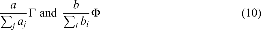
Similar to Equation (7), an additional row can be projected as a supplementary point in an existing CA plot. Let the extra row (supplementary) point be the vector $a = [a_{1}, a_{2}, \dots, a_{J}]$ and an extra column (supplementary) point be the vector $b = [b_{1}, b_{2}, \dots, b_{I}]$ . The projections for the row point a and the column point b are found by

\frac{a}{\sum_{j} a_{j}} Γ and \frac{b}{\sum_{i} b_{i}} Φ

(10)

respectively. These supplementary points do not determine the CA solution, but from these projections we can see the relationships between the configurations of row and column points in the existing CA solution to these supplementary points.

To summarize how to obtain CA solution, there are three steps (Qi et al., 2024). Step 1: compute the matrix of standardized residuals $D_{r}^{- 1 / 2} (P - E) D_{c}^{- 1 / 2}$ ; Step 2: compute the SVD of the matrix $D_{r}^{- 1 / 2} (P - E) D_{c}^{- 1 / 2} = U Σ V^{T}$ ; Step 3: obtain standard coordinates for rows $Φ = D_{r}^{- 1 / 2} U$ and for column $Γ = D_{c}^{- 1 / 2} V$ and obtain principal coordinates for rows $F = Φ Σ$ and for columns $G = Γ Σ$ . In this paper, we use the principal coordinates for rows and columns to make CA plot. We use visual inspection of the CA plot to define outlying cells. A cell is an outlying cell if the corresponding row and column points of this cell lie far from other points.

We now analyze the attributes of brands of cars dataset to illustrate CA. The dataset has been analysed before in Raymaekers and Rousseeuw (2024); Riani et al. (2022). This dataset is a part of the R package cellWise (Raymaekers, Rousseeuw, Van den Bossche, & Hubert, 2023). See Table 1 for the data. The contingency table consists of 39 rows and 7 columns. The rows represent 39 brands of cars, such as Jeep, Porsche, and Volvo. The seven columns represent the attributes: Fuel Economy, Innovation, Performance, Quality, Safety, Style, and Value. In total 1,578 participants were asked what they considered attributes for the 39 different vehicle brands. They selected all attributes in the list which they felt applied to a brand. An entry in the table represents the number of respondents that chose the attribute for a car. In total this led to 11,713 scorings. We note that this is not a typical contingency table as in a typical table the total count is identical to the number of respondents.

Table 1.

Car data matrix

	Fuel Econo.	Innov.	Perform.	Quality	Safety	Style	Value	Total	Proport.
Acura	24	38	28	20	28	33	25	196	0.017
Audi	9	54	54	30	19	67	8	241	0.021
Bentley	0	16	18	25	9	27	17	112	0.010
BMW	14	83	94	55	38	93	35	412	0.035
Buick	25	48	39	58	52	52	43	317	0.027
Cadillac	14	73	50	76	40	83	36	372	0.032
Chevrolet	114	103	202	174	140	160	145	1,038	0.089
Chrysler	38	65	96	54	54	103	72	482	0.041
Dodge	60	61	141	61	63	133	69	588	0.050
Ferrari	0	20	45	10	8	46	5	134	0.011
Fiat	19	21	17	20	15	7	16	115	0.010
Ford	167	180	169	179	161	157	188	1,201	0.103
GMC-trucks	40	40	64	57	80	50	58	389	0.033
Honda	163	68	73	118	104	50	135	711	0.061
Hyundai	97	25	31	27	35	42	82	339	0.029
Infiniti	5	39	31	15	10	17	16	133	0.011
Jaguar	0	3	18	19	3	47	12	102	0.009
Jeep	18	33	14	51	19	41	52	228	0.019
Kia	68	30	17	13	24	42	109	303	0.026
Lamborghini	5	19	37	8	6	23	24	122	0.010
Land-Rover	0	43	0	5	0	47	2	97	0.008
Lexus	10	62	29	50	27	64	26	268	0.023
Lincoln	6	37	23	31	24	40	19	180	0.015
Maserati	0	6	9	0	0	41	25	81	0.007
Mazda	46	23	34	10	12	26	38	189	0.016
Mercedes-Benz	8	83	44	87	58	82	42	404	0.034
Mini	23	12	4	4	13	12	4	72	0.006
Mitsubishi	20	13	33	23	7	32	13	141	0.012
Nissan	80	68	51	53	52	55	70	429	0.037
Porsche	0	17	66	14	6	42	5	150	0.013
Ram-trucks	9	22	21	10	18	1	16	97	0.008
Rolls-Royce	0	4	4	35	11	25	17	96	0.008
Scion	20	24	11	6	11	4	4	80	0.007
Smart	38	9	3	7	0	5	10	72	0.006
Subaru	19	14	32	33	75	20	40	233	0.020
Tesla	23	35	10	12	9	15	12	116	0.010
Toyota	238	116	95	134	113	74	150	920	0.079
Volkswagen	90	30	25	37	27	22	46	277	0.024
Volvo	9	15	16	31	180	14	11	276	0.024
Total	1,519	1,652	1,748	1,652	1,551	1,894	1,697	11,713
Proport.	0.130	0.141	0.149	0.141	0.132	0.162	0.145		1.000

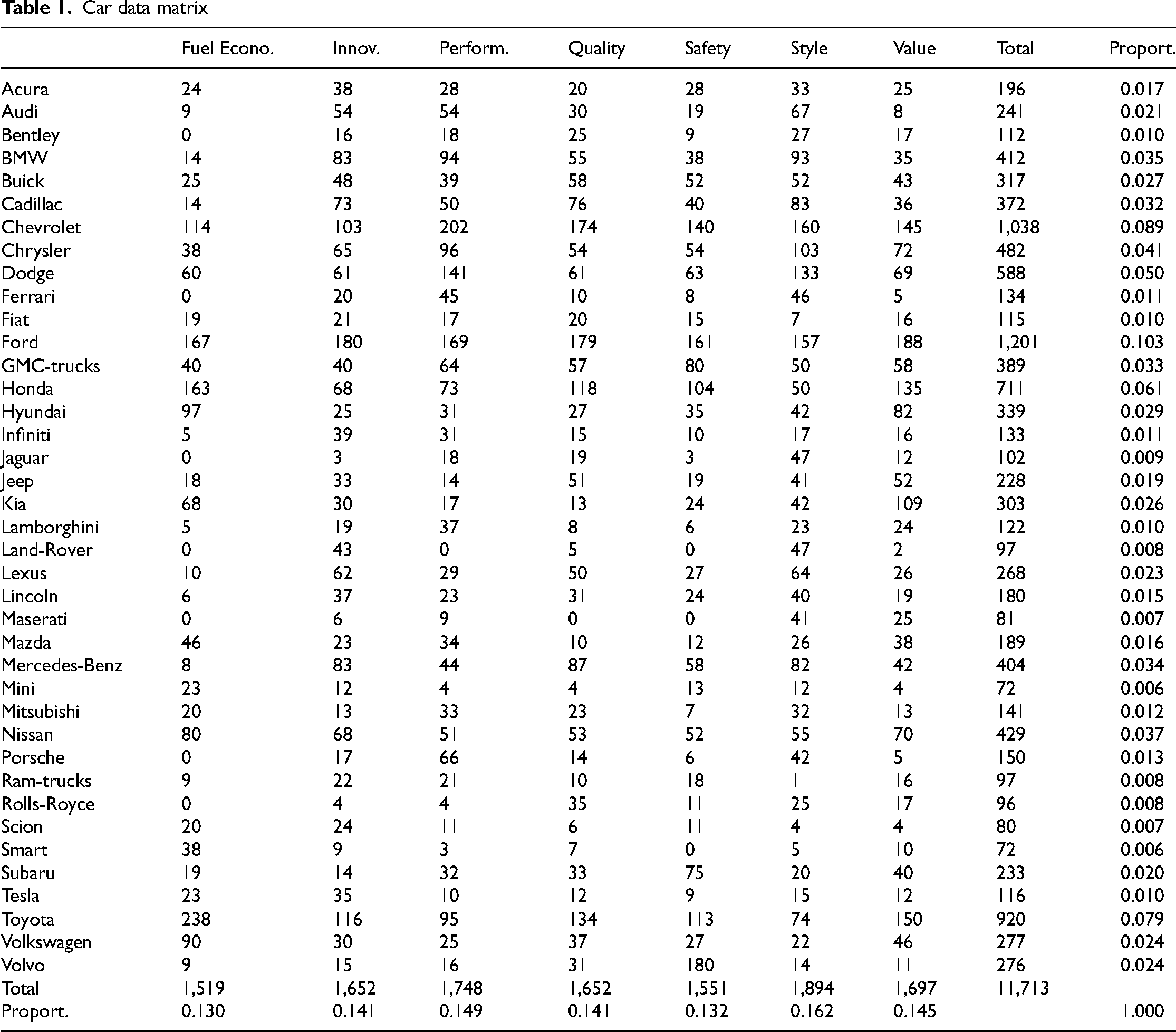
Figure 1 shows the symmetric plot of CA, having $F_{2}$ and $G_{2}$ as coordinates. The first two singular values, with percentage of inertia displayed between brackets, are 0.335 (41.3%) and 0.281 (28.9%). The first dimension contrasts cars that score high on Fuel Economy versus cars that score high on Style and Performance. On the second dimension the car brand Volvo is far from other brands of cars, and the attribute Safety is close by. Where the marginal proportion of Volvo is 0.024, its contribution to the second dimension is 65.7%. For Safety the marginal proportion is 0.132, but the contribution to the second dimension is 75.2%. In addition, the contribution of cell (Volvo, Safety) to the total inertia is 17.7%. Hence the cell (Volvo, Safety) is a cell-wise outlier, leading to outlying points for Volvo and Safety on dimension 2. In Supplementary materials A, we enumerate three potential causes for the presence of outliers.

Figure 1.

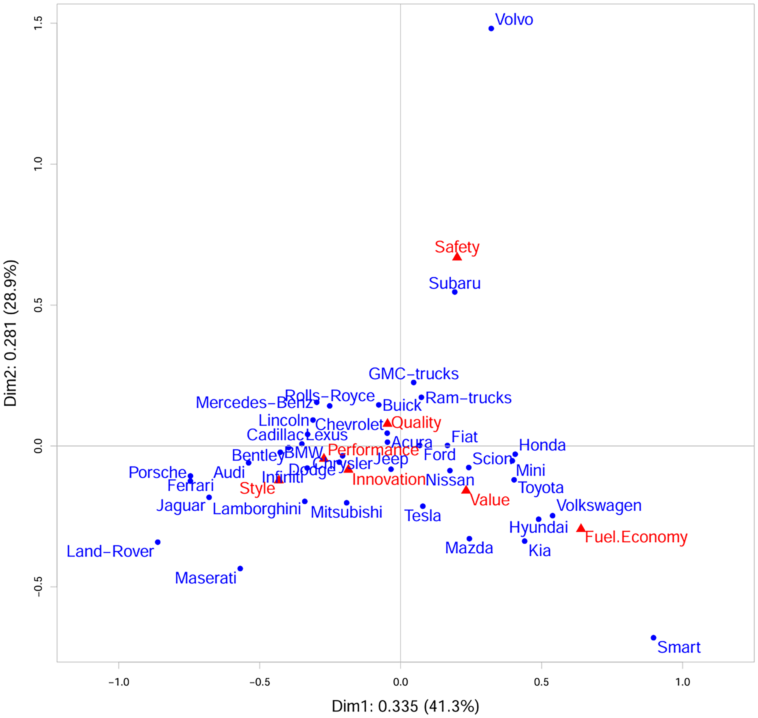
CA plot of Table 1

Methods to handle outliers

We discuss three methods to handle outliers. Two methods are cell-wise outlier methods: reconstitution of order h and MacroPCA. The third is the supplementary points method. It is worth noting that reconstitution of order h has been used to handle missing data, but has not been proposed to handle outliers.

Reconstitution of order $h$

In this paper we propose to deal with an outlier or outliers by changing the data. Specifically, we assume that specific cells in a matrix are outlying cells if they cause row and column points to be outliers. We propose to make such cells in the data matrix missing. We use visual inspection of the CA plot to define outlying cells. In a second step, we apply an algorithm that imputes a new value for each missing value. For this, we use the reconstitution algorithm, originally proposed by Nora-Chouteau (1974) and revisited by Greenacre (1984), De Leeuw and Van der Heijden (1988), and Josse et al., (2012).

We assume for the moment that there is only a single cell causing a row and a column to be outliers, but the procedure that we describe can be applied to multiple outlying cells simultaneously. The idea is to adjust the value in this single cell in such a way that it is perfectly reconstituted in a $h$ -dimensional CA solution. This reconstitution is obtained iteratively.

Since the margins vary as the missing cell is iteratively imputed, it is easier to describe the method using the raw data $x_{i j}$ instead of the proportions $p_{i j}$ . For $x_{i j}$ we have

x_{i j} = \frac{x_{i +} x_{+ j}}{x_{+ +}} (1 + \sum_{k = 1}^{\min {I - 1, J - 1}} ϕ_{i k} σ_{k} γ_{j k}),

(11)

i.e.

x_{i j}

is reconstituted if the maximum dimensionality min

(I - 1, J - 1)

is used. Let

{\hat{x}}_{i j}

be the reconstituted value using

h <

min

(I - 1, J - 1)

dimensions. Then

{\hat{x}}_{i j} = \frac{x_{i +} x_{+ j}}{x_{+ +}} (1 + \sum_{k = 1}^{h} ϕ_{i k} σ_{k} γ_{j k}) .

(12)

We first explain reconstitution of order 0, meaning that no CA dimensions are used in the reconstitution. Assume that cell $(m, n)$ is an outlier made missing, and assume that at iteration $t = 0$ we impute a non-negative value. Then we iteratively find updates for this missing value as follows:

x_{m n}^{t + 1} = \frac{x_{m +}^{t} x_{+ n}^{t}}{x_{+ +}^{t}} .

(13)

After convergence, we have the converged value $x_{m n} *$ (De Leeuw & Van der Heijden, 1988). Then CA is applied to the original data where the outlier value in cell $(m, n)$ is replaced by $x_{m n} *$ . As $x_{m n} * = x_{m +} * x_{+ n} * / x_{+ +} *$ , in Equation (11) the residual for cell $(m, n) x_{m n} * - x_{m +} * x_{+ n} * / x_{+ +} * = 0$ . In this sense, the influence of the original outlying cell is eliminated. De Leeuw and Van der Heijden (1988) use reconstitution of order zero in the context of the statistical quasi-independence model. They adjust CA so that it can decompose the departure from this model, a model that assumes independence for some but not all cells in a contingency table. Reconstitution of order zero is available in the R Package anacor (De Leeuw & Mair, 2009).

However, as the residual for cell $(m, n)$ is 0, the inner-product $\sum_{k = 1}^{\min {I - 1, J - 1}} ϕ_{m k} * σ_{k} * γ_{n k} * = 0$ as well, meaning that in the full-dimensional space the vectors m and n are orthogonal. This may be an undesirable bi-product of reconstitution of order 0. An alternative, reconstitution of order h, does not have this problem. In reconstitution h, the value in cell $(m, n)$ is reconstituted by

x_{m n}^{t + 1} = \frac{x_{m +}^{t} x_{+ n}^{t}}{x_{+ +}^{t}} (1 + \sum_{k = 1}^{h} ϕ_{m k}^{t} σ_{k}^{t} γ_{n k}^{t}) .

(14)

Thus the first h dimensions of CA for row m and column n are given by $ϕ_{m k} *$ , $σ_{k} *$ , $γ_{n k} *$ , $k = 1, 2, \dots, h$ and then the value in the cell $(m, n)$ is reconstituted perfectly by the first h dimensions of CA ( $x_{m, n} * = (x_{m +} * x_{+ n} * / x_{+ +} *) (1 + \sum_{k = 1}^{h} ϕ_{m k} * σ_{k} * γ_{n k} *)$ ). The residual as well as inner-product for higher dimensions than h for cell $(m, n)$ is 0, namely, $\sum_{k = h + 1}^{m i n {I - 1, J - 1}} ϕ_{m k} * σ_{k} * γ_{n k} * = 0$ . This means that the parameters $ϕ_{i k}$ , $σ_{k}$ , and $γ_{j k}$ , $k = 1, 2, \dots, h$ provide the CA solution based on the non-outlying cells in the matrix only. Therefore, when we are interested in the first h dimensions of the CA solution, it is theoretically advantageous to use the reconstitution of order h, thereby ensuring that the cell-wise outlier has no influence on the first h dimensions of CA. So, when interest goes out to a CA solution of two dimensions, theoretically it makes sense to eliminate the influence of an outlier by applying reconstitution of order 2. However, in practice this may lead to a negative value for $x_{m, n} *$ , as is the case in the second example of Empirical Section. In such instances reconstitution of order zero is the preferred option.

As far as we know, there is no R package in which reconstitution of order h is implemented, where $h \geq 1$ . We present the R function reconca, that we created by rewriting the function imputeCA taken from the R package missMDA. The function imputeCA implements a regularized reconstitution algorithm (Josse et al., 2012; Josse & Husson, 2016) that is meant for the missing value problem where the number of missing values in the data is relatively large. This is a situation different from our idea to make outlying values missing and therefore we further ignore this regularized version in this paper.

MacroPCA

MacroPCA was originally proposed for PCA (Hubert et al., 2019) and subsequently adjusted for CA (Raymaekers & Rousseeuw, 2024). MacroPCA is quite involved and detects outliers and handles outliers at the same time. It includes two parts. The first part of MacroPCA is a multivariate method called DetectDeviatingCells (DDC) (Hubert et al., 2019; Rousseeuw & Van Den Bossche, 2018) that assumes that data are generated from a multivariate Gaussian distribution but some cells were corrupted. DDC detects cellwise outliers, and provides these cellwise outliers with initial values. It also detects initial row-wise outliers. In the second part, the set of outlying rows will be improved. Low-dimensional representations are obtained in a way that is similar but not identical to the reconstitution algorithm. The low-dimensional representations of MacroPCA are not nested. That is, for example, the two-dimensional representation is not a subset of three-dimensional representations. We refer to Hubert et al. (2019); Rousseeuw and Van Den Bossche (2018) for details.

MacroPCA is modified to handle missing data and outlier problems in the context of CA (Raymaekers & Rousseeuw, 2024). For CA the original matrix is replaced with the matrix of standardized residuals. As in CA the standardized residuals are only a starting point in finding the CA solution, the modification is close to but different from CA. Also, in the DCC step of MacroPCA where outlying cells are detected, the algorithm makes the assumption of a Gaussian distribution, for which there is no clear rationale in the context of CA.

Supplementary points method

The supplementary points method is a well-known method to deal with row-wise outliers or column-wise outliers. That is, after noticing outlying points, for which we use visual inspection, a new CA is performed on the data matrix where these row-wise or column-wise outliers are removed. Then, as a second step, these outliers are projected as supplementary points into the existing CA solution. Using Equation (10) in CA background section, if an outlier a is a row point, its coordinates in the $K$ -dimensional CA solution are given by $(a / \sum_{j} a_{j}) Γ_{K}$ and if an outlier b is a column point, its coordinates in the $K$ -dimensional CA solution are given by $(b / \sum_{i} b_{i}) Φ_{K}$ .

The supplementary points method is a standard method to deal with outliers in CA, see, for example, Hoffman and Franke (1986), Bendixen (1996), Greenacre (2017), and Riani et al. (2022). However, as we argued in Section Introduction, outliers may be caused by a single cell in the data matrix, and deleting an entire row or column where cell-wise outliers occur from the contingency table leads to a loss of the entire category, including outlying and non-outlying cells. In contrast, reconstitution of order h eliminates the effect of only the outlying cells, thus keeping as much information as possible in the analysis.

Experimental studies

Here, we show the results of some experimental studies to evaluate different outlier handling methods. To create a contingency table, we first specify the marginal probabilities and CA dimensions and then use the reconstitution formula (9). For the cell-wise outlier, we set an element in the table to be large. We study three scenarios. Namely, we create a contingency table based on Equation (9) where the dimensionality K of the CA solution is 0, 1 and 2. All tables (Table B.1, Table B.2, and Table B.3) for this Section can be found in the Supplementary materials.

Dimensionality is 0

A contingency table with dimensionality 0 is created by the marginal probabilities $p_{i +}$ and $p_{+ j}$ . First, we randomly generate row marginal probabilities $p_{i +}$ , $i = 1, 2, \dots, I$ , which follow a uniform distribution U(0, 1), and we normalize them such that $\sum_{i} p_{i +} = 1$ . Similarly for column marginal probabilities $p_{+ j}$ , $j = 1, 2, \dots, J$ . Joint probabilities $p_{i j}$ are found by $p_{i j} = p_{i +} p_{+ j}$ . We cannot perform CA on this matrix because the elements follow statistical independence.

For our experimental studies we take $I = 5$ and $J = 6$ . The rows of tables are ordered from 1 to 5 and the columns from a to f. The (rounded) generated row marginal probabilities are (0.040, 0.220, 0.215, 0.220, 0.304) and column marginal probabilities are (0.232, 0.003, 0.084, 0.242, 0.187, 0.252). The matrix of joint probabilities is in Table B.1a.

A cell-wise outlier in cell (1,a)

To create a contingency table with a cell-wise outlier, we set the element $p_{1 a} = 4 \times \max$ ${p_{1 a}, \cdot \cdot \cdot, p_{5 f}} = 4 \times 0.07656 = 0.30625$ and then obtain Table B.1b which is the same as Table B.1a except for element $p_{1 a}$ . We rescale the elements of Table B.1b so that they add up to 1 and calculate a CA solution.

The CA solution only has one dimension. Figure 2 shows the symmetric plot of CA based on Table B.1b. In Figure 1, row 1 and column a, where the outlying cell is located, are far from other points. The singular value, with percentage of inertia displayed between brackets, is 0.603 (100%). We analyze the contribution of row 1 and column a to the first dimension. The marginal proportion of row 1 is 0.260, yet its contribution to the first dimension is 74.0%; the marginal proportion of column a is 0.408, yet its contribution to the first dimension is 59.2%. The contribution of cell (1, a) to the total inertia is 43.8%.

Figure 2.

CA plot about Table B.1b with outlier (1,a)

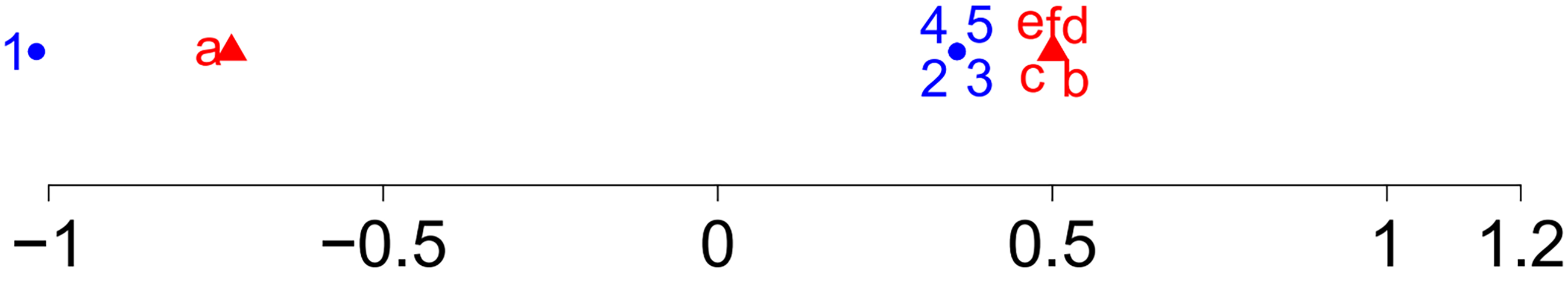
Reconstitution of order 0 - We use reconstitution of order 0 to handle the cell-wise outlier (1, a). Using the reconstitution algorithm, the value 0.30625 in (1, a) becomes 0.00934, the same as in Table B.1a. Thus the elements in the table are independent. We conclude that reconstitution of order 0 works well.

Dimensionality is 1

A contingency table is created by the marginal probabilities, row scores $ϕ_{i 1}$ and column scores $γ_{j 1}$ in dimension 1, and the first singular value $σ_{1}$ . We take the same row and column marginal probabilities as in precedent Subsection. Second, we take row scores $ϕ_{i 1}$ as normalized values of (1, 2, 3, 4, 5) and column scores $γ_{j 1}$ as normalized values of (1, 2, 3, 4, 5, 6) satisfying Equations (4) and (5). The first singular value is set to be 0.42. Joint probabilities are established by the reconstitution formula in Equation (9).

The matrix of joint probabilities is given in Table B.2a. We perform CA on this matrix and obtain Figure 3a. As intended, the CA solution only has one dimension. Row points are ordered from 1 to 5, column points from a to f.

Figure 3.

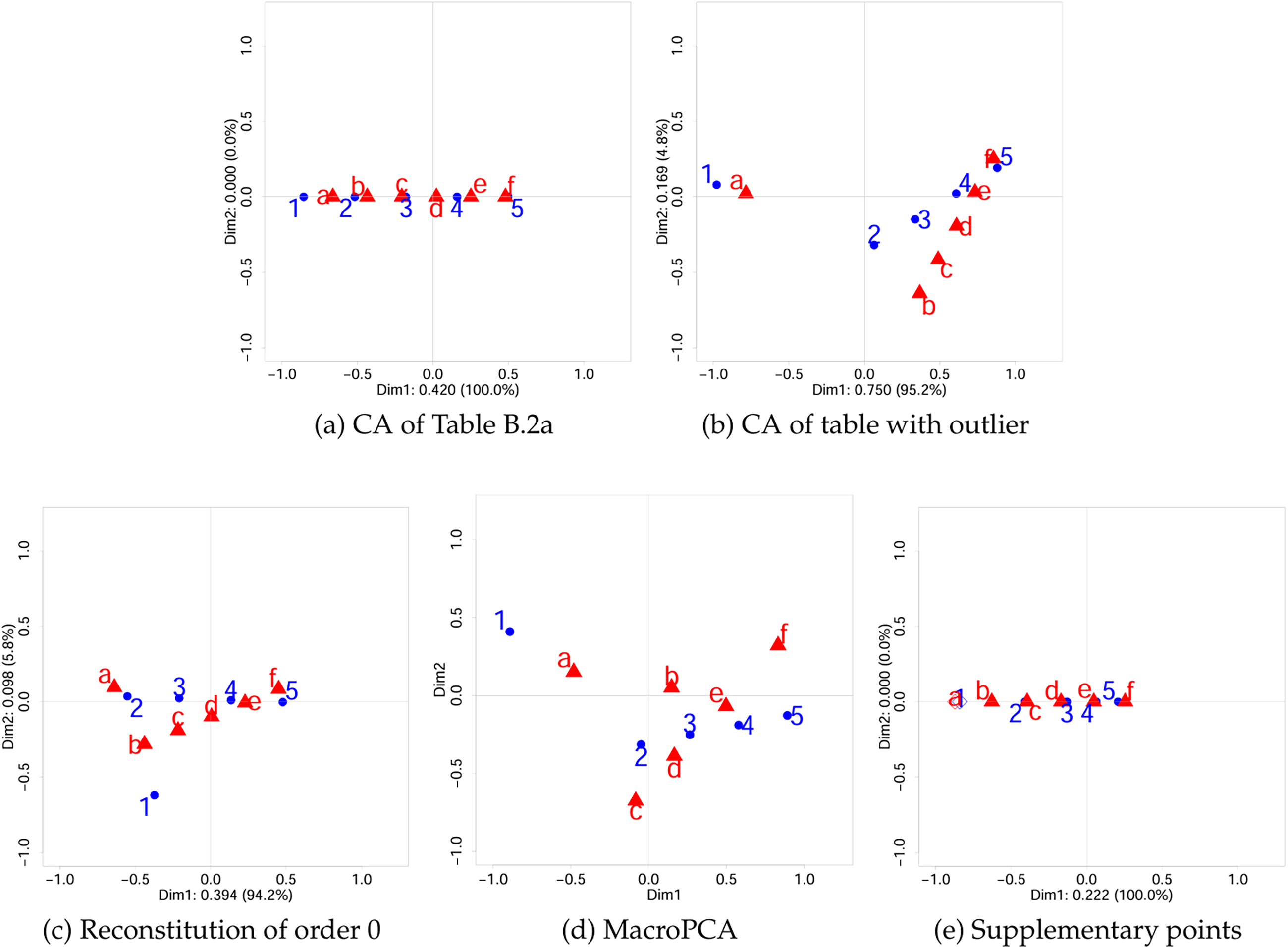
(a) CA of Table B.2a, (b) CA of table with outlier, (c) Reconstitution of order 0, (d) MacroPCA, and (e) Supplementary points

A cell-wise outlier in cell (1,a)

To create a contingency table with a cell-wise outlier, we let the element $p_{1 a} = 4 \times \max {p_{1 a}, \cdot \cdot \cdot, p_{5 f}} = 4 \times 0.12015 = 0.48060$ , and then we obtain Table B.2b, which is the same as Table B.2a except $p_{1 a}$ .

The CA solution has two dimensions. Figure 3b shows the symmetric plot of CA based on Table B.2b. Compared with Figure 3a, the first dimension in Figure 3b shows that the order of row points and column points remains the same. However, the outliers row 1 and column a are far from other points and lie on one side of the origin, and a second dimension is needed. The first two singular values, with percentage of inertia displayed between brackets, are 0.74970 (95.2%) and 0.16883 (4.8%).

Reconstitution of order 0, 1, and 2 - First we use the reconstitution of order 0 to handle the cell-wise outlier (1, a). Using the reconstitution algorithm, the value 0.48060 in (1, a) becomes 0.00511 which is similar but not identical to 0.02196 in Table B.2a.

We perform CA on this matrix and obtain Figure 3c, whose first dimension is similar with the first dimension of Figure 3a except that row 1 is larger than row 2. We note that, as the reconstituted value in cell (1, a) is the product of the row and column margins $p_{11} = p_{1 +} p_{+ 1}$ , the residual $p_{11} - p_{1 +} p_{+ 1} = 0$ . Thus, row 1 with coordinate $(ϕ_{11} σ_{1}, ϕ_{12} σ_{2})$ and column a with coordinate $(γ_{11}, γ_{12})$ are orthogonal in an asymmetric map. Here we have a symmetric map, so there is approximate orthogonality. The contribution of element (1, a) to total inertia is 0.

Now we use the reconstitution of order 1 to handle the cell-wise outlier. Using the reconstitution algorithm, the value 0.48060 in (1, a) becomes 0.02196, which is the same as the value in Table B.2a. So here the reconstitution algorithm works as intended.

We also use reconstitution of order 2, and the imputed value is the same as the initial in the reconstitution algorithm. This is because the CA solution has two dimensions. The outlier in cell (1, a) in Table B.2b is perfectly reconstituted by order 2. So if h is taken too large, the reconstitution algorithm is not able to eliminate the impact of the outlier.

MacroPCA - We obtain the results of MacroPCA by applying the MacroPCA function in the R package cellWise (Raymaekers et al., 2023). We use the same parameter setting as in the car dataset of Raymaekers and Rousseeuw (2024) and Raymaekers et al. (2023), except for $α = 0.8$ and $k = 2$ (compare Software availability in Raymaekers and Rousseeuw (2024)). By setting $α = 0.8$ we make the number of non-outlying rows as large as possible.

Figure 3d is the corresponding symmetric CA-type plot based on MacroPCA. MacroPCA does not work well, as in the first dimension the order of the columns is not reproduced. For more details, see the Supplementary materials B.2.1.

Supplementary points method - Here we use the supplementary points method to deal with outliers 1 and a. We treat 1 and a as supplementary points. Thus the table analysed has size 4 × 5, and now, row 1 and column a have no effect on the solution of CA. The singular value, with percentage of inertia displayed between brackets, is 0.22243 (100%).

Figure 3e shows a symmetric CA plot, where 1 and a are added as supplementary points. The order of row and column points is the same as the order in the original Figure 2a. So here the supplementary points method works well.

Dimensionality is 2

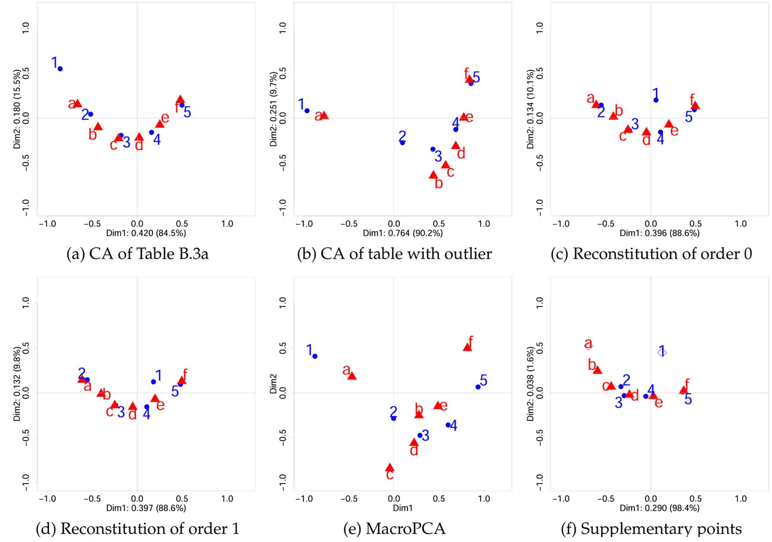
We use the same matrix as the matrix for dimensionality is 1, but now we add a second dimension. I.e. we take row scores $ϕ_{i 2}$ for dimension 2 as normalized squared values of dimension 1 satisfying Equations (4) and (5), and similarly for the column scores $γ_{j 2}$ . The second singular value is set to 0.18. The matrix of joint probabilities is given in Table B.3a. We perform CA on this matrix and obtain Figure 4a. As intended, the CA solution has two dimensions. The first two singular values, with percentage of inertia displayed between brackets, are 0.420 (84.5%) and 0.180 (15.5%).

Figure 4.

(a) CA of Table B.3a, (b) CA of table with outlier, (c) Reconstitution of order 0, (d) Reconstitution of order 1 (e) MacroPCA, and (f) Supplementary points

A cell-wise outlier in cell (1, a)

To create a contingency table with a cell-wise outlier, again, we let the element $p_{1 a} = 4 \times \max {p_{1 a}, \cdot \cdot \cdot, p_{5 f}} = 4 \times 0.13256 = 0.53025$ and then obtain Table B.3b which is the same as Table B.3a except $p_{1 a}$ .

The CA solution has three dimensions. Figure 4b shows the symmetric plot of CA based on Table B.3b. In the first dimension, the outliers row 1 and column a are far from other points. The first three singular values, with percentage of inertia displayed between brackets, are 0.76415 (90.2%), 0.25057 (9.7%), and 0.02844 (0.1%).

Reconstitution of order 0, 1, and 2 - We use the reconstitution of order 0 to handle the cell-wise outlier (1, a). The value 0.53025 in (1, a) becomes 0.00379, similar but not identical to 0.02633 in Table B.3a. We perform CA on this matrix and obtain Figure 4c. Figure 4c is similar with Figure 4a except that row point 1 is close to the origin.

Now we use reconstitution of order 1. Using the reconstitution algorithm, the value 0.53025 in (1, a) becomes 0.00252, similar but not identical to 0.02633 in Table B.3a. We perform CA on this matrix and obtain Figure 4d, which is similar with Figure 4c.

Last, we use reconstitution of order 2 to handle the cell-wise outlier (1, a). Now the value 0.53025 in (1, a) becomes 0.02633, which is the same value as in Table B.3a. Therefore, the reconstitution of order 2 works perfectly.

MacroPCA - Here we use the same parameter setting as in Subsection “Dimensionality is 1”. Figure 4e is the corresponding symmetric CA-type plot based on MacroPCA. MacroPCA does not work well, as the order of the columns is not reproduced in the first dimension of the figure. For more details, see the Supplementary materials B.3.1.

Supplementary points method - Here we treat 1 and a as supplementary points. Thus the table analysed has size 4 × 5, and now, row 1 and column a have no effect on the solution of CA. The first two singular values, with percentage of inertia displayed between brackets, are 0.29050 (98.35%), 0.03762 (1.65%). Figure 4f shows a symmetric CA plot, where 1 and a are added as supplementary points. The supplementary points method works fine for the column points but not for the row points.

Conclusion

In this section, we performed some experimental studies. We explored the choice of the parameter h in the reconstitution algorithm. It appears that an optimal choice of h depends on how a contingency table is constructed. If a contingency table is constructed by the h dimensions of CA and then cells in the table are contaminated as outliers, reconstitution of order h works perfectly.

Reconstitution of order h clearly outperforms MacroPCA. In the examples we studied, reconstitution of order h did better than the supplementary points method where dimensionality is 2. In the examples where dimensionality is 1, reconstitution of order 0 is less appealing than the supplementary points method in terms of the order of row points, but the reconstitution of order 1 works perfectly.

Yet more study is needed to better understand the behavior of reconstitution of order h. The choice for the experimental data is quite limited. In the Supplementary materials more results can be found, for the situation that cell (1,c) is an outlier.

Empirical studies

We consider two datasets, the attributes of brands of cars (analysed before in CA background section) and ocean plastic datasets. The attributes of brands of cars dataset is a classic dataset to study the problem of outliers in the context of CA (Raymaekers & Rousseeuw, 2024; Riani et al., 2022). For example, Raymaekers and Rousseeuw (2024) use the dataset to explore the usefulness of MacroPCA in terms of outliers in CA. Therefore we compare reconstitution of order h, MacroPCA, and the supplementary points method on this dataset.

The ocean plastic dataset is an incidence dataset created by Vonk et al. (2024). We use this dataset to show that the reconstitution algorithm is appropriate for incidence data as well. However, we do not discuss MacroPCA for this example, as MacroPCA applied to this dataset yielded a degenerate solution (See Supplementary C in the Supplementary materials). The reason for this is not clear to us, but we notice that assumptions underlying MacroPCA are severely violated by the matrix of standardized residuals. Therefore, for this dataset, we only compare reconstitution of order h and the supplementary points method.

The attributes of brands of cars data

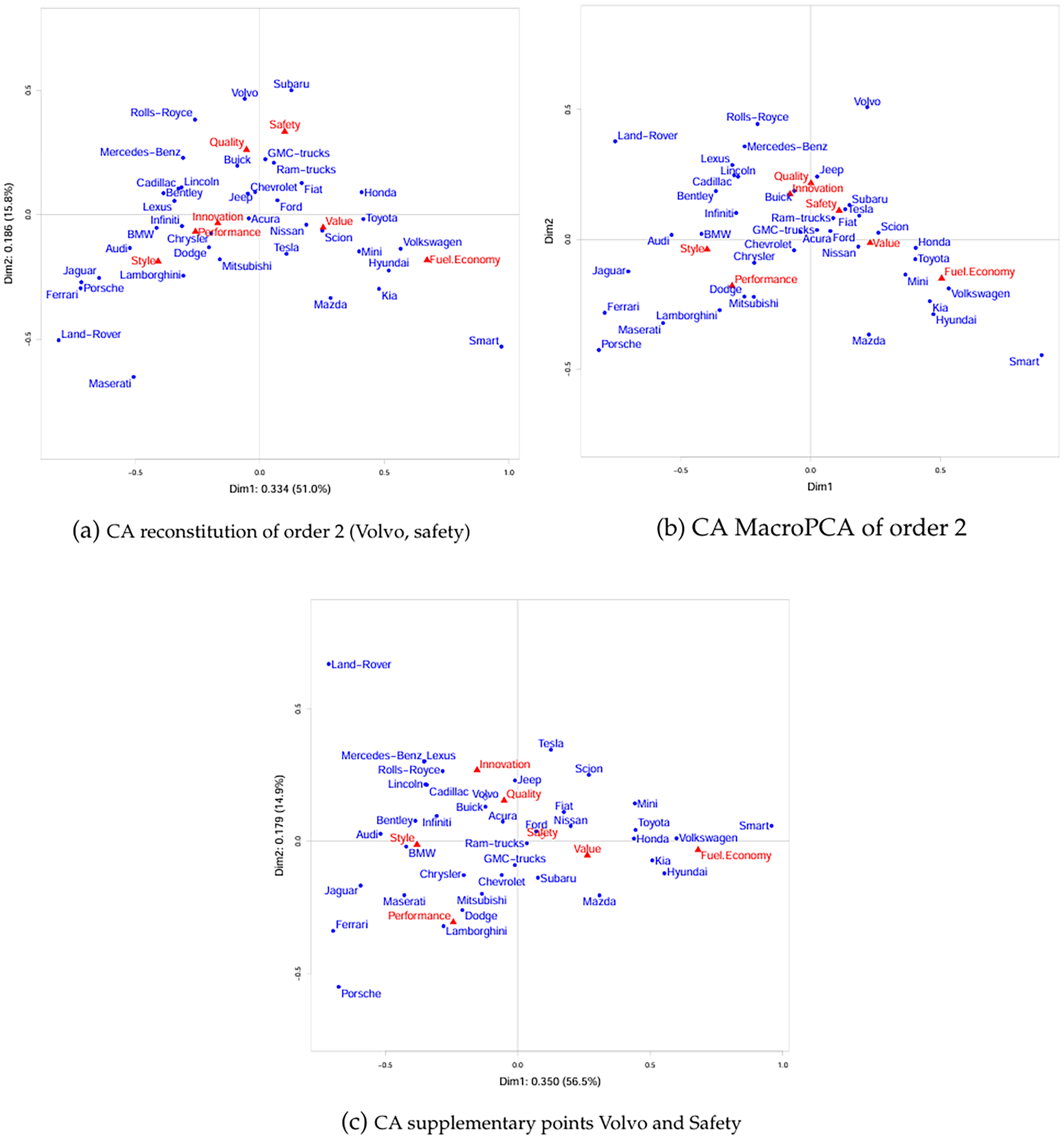
As a first dataset, we use the attributes of brands of cars dataset to illustrate our method. We analysed this dataset before in CA background section. From this section, we concluded that the cell (Volvo, Safety) is a cell-wise outlier, leading to outlying points for Volvo and Safety on dimension 2.

Reconstitution algorithm

Here we use reconstitution algorithm of order 2 to handle the cell-wise outlier (Volvo, Safety). Using the reconstitution algorithm, the value 180 in (Volvo, Safety) becomes 27.0 (Reconstitution of order 0 leads an imputed value of 13.1, but the graphic results are similar). The contribution of cell (Volvo, Safety) to the total inertia went down from 17.7% to 0.4%. The first four singular values become 0.334 (51.0%), 0.186 (15.8%), 0.170 (13.2%), and 0.156 (11.1%). It is clear that the second dimension now is less important, the proportion of inertia went down from 28.9% to 15.8%. The singular values of dimensions 2, 3 and 4 do not differ much, and using the elbow criterion, we decide only to study the first dimension. Also, since in a contingency table the singular value can be interpreted as the canonical correlation between the row variable and the column variable, with 0.186 the second singular value is quite small.

Figure 5a is a symmetric CA plot of the reconstituted table. On the first dimension the configuration of row and column points is similar to the configuration of the original Figure 1, except for the change of location of Volvo. Safety is still in a similar position, and the reason for this difference between Volvo and Safety is that bringing down the value of 180 to 27 has a much larger impact on the profile of Volvo, that originally had a marginal total of 276, than the marginal total of Safety, that originally was 1,551. Note that by eliminating the impact of a single cell the new figure is much better readable than Figure 1.

Figure 5.

CA plots about Car dataset

By eliminating the influence of a single cell the reconstitution method allows us to arrive at the simple conclusion that (i) there is a single outlying cell for Volvo and Safety, as Safety is chosen as the outstanding characteristic of Volvo (180 out of 276 scores for Volvo come from Safety), and (ii) there is largely a one-dimensional structure for the cars and features going from Land-Rover, Ferrari and Porsche on the left, scoring higher than average on Style and Performance, to Smart, Volkswagen, Hyundai and Kia, on the right, scoring higher on Fuel Economy, with the other car types and features ordered in between.

MacroPCA

We obtain the results of MacroPCA by applying the MacroPCA function in the R package cellWise (Raymaekers et al., 2023). We use the same parameter setting as in Raymaekers and Rousseeuw (2024) and Raymaekers et al. (2023), except for $α = 0.97$ and $k = 2$ . By setting $α = 0.97$ we make the number of non-outlying rows as large as possible. We choose $k = 2$ because this simplifies the comparison with the reconstitution of order $h = 2$ in CA.

The results from the first step in MacroPCA, DCC, provides a cellmap. See Figure 6. The red or blue cells indicate cellwise outliers. Specifically, red cells indicate that the observed values are much larger than the predicted values, and for blue cells the opposite holds. Thus DDC finds 19 cellwise outliers, including the cellwise outlier (Volvo, Safety) found using the visual inspection employed in precedent “Reconstitution algorithm” Section.

Figure 6.

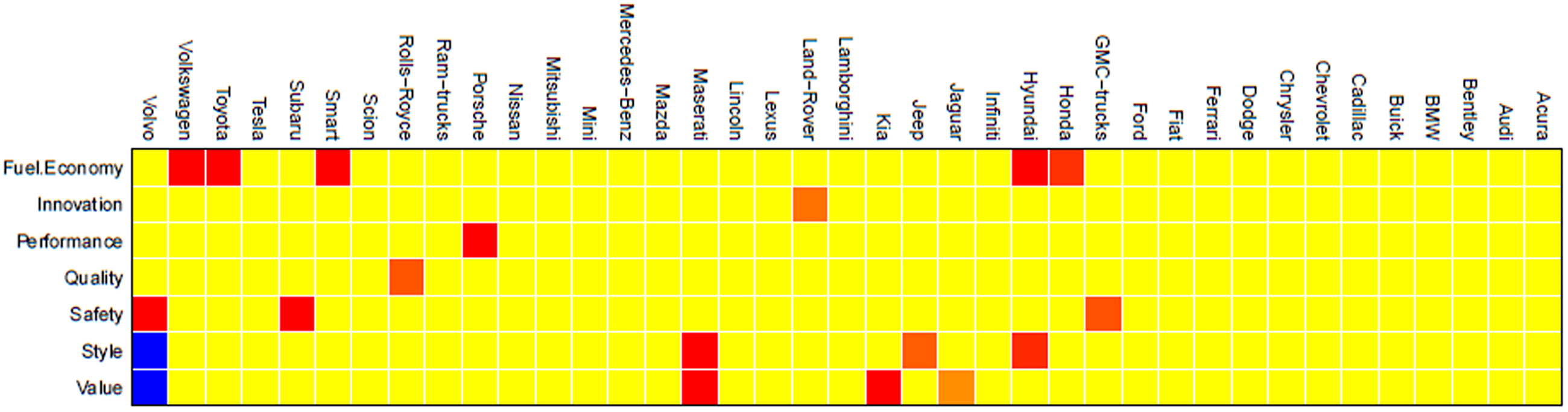
Cellmap from DDC of MacroPCA about Car dataset to detect cell-wise outliers

Figure 5b is the corresponding symmetric CA-type plot. On the first dimension, the configuration of row and column points is similar to the original Figure 1.

Supplementary points method

From CA background section, we concluded that Volvo and Safety are far from other points and coined Volvo and Safety outliers. Therefore, we handle Volvo and Safety as supplementary points. Thus the table analysed has size $38 \times 6$ , and now, row Volvo and column Safety have no effect on the solution of CA but are projected into it afterwards. The first four singular values are 0.350 (56.5%), 0.179 (14.9%), 0.166 (12.7%), and 0.150 (10.3%). As in the reconstitution approach, the second dimension is now less important, the proportion of inertia went down from 28.9% to 14.9%, and using the elbow criterion, only the first dimension is to be studied.

Figure 5c shows a symmetric CA plot, where Volvo and Safety are added as supplementary points. On the first dimension the configuration of row and column points is similar to the original Figure 1, except for Volvo. Again, Safety is still in a similar position. For this dataset the interpretation using the supplementary points method is very similar to the interpretation using the reconstitution approach.

The ocean plastic data

The ocean plastic dataset is created by Vonk et al. (2024) to analyze how scientific studies on ocean plastic are communicated in press releases. The study analyzed press releases published on EurekAlert! between January 2017 and December 2021. In the analysis, variables defining the four frame elements of Entman (1993), namely causal interpretation, problem definition, moral evaluation, and treatment recommendation were noted, resulting in 21 frame variables. Table 2 summarizes these framing variables, while a more detailed description can be found in Appendix 1 of Vonk et al. (2024).

Table 2.

Frame variables

CCC	Cause: Ocean climate change	PH	Health
Resp.C.P	Actor responsible for cause: Politics	PE	Economic
Resp.C.I	Actor responsible for cause: Industry	PB	Biological
Resp.C.C	Actor responsible for cause: Regions/Countries	PnB	Non-Biological
Resp.C.S	Actor responsible for cause: Society	PT	Treatment
Resp.C.O	Actor responsible for cause: Other	PC	Conflict
		OC	Opportunity
(a) Causal interpretation		(b) Problem definition
Tr	Treatment recommendation	OT	Opportunity due to treatment
(c) Treatment recommendation		Resp.T.P	Actor responsible for treatment: Politics
		Resp.T.I	Actor responsible for treatment: Industry
		Resp.T.C	Actor responsible for treatment: Region/Countries
		Resp.T.S	Actor responsible for treatment: Society
		Resp.T.O	Actor responsible for treatment: Other
		Ur	Urgency to take action
		(d) Moral evaluation

The causal interpretation (a) was coded, when the text referred to climate change (CCC) as a cause of problems. It was coded whether an entity was held responsible for causing climate change, ocean plastics or related problems (Resp.C.P, Resp.C.I, Resp.C.C, Resp.C.S, and Resp.C.O). The problem definition (b) describes different problems (PH, PE, PB, PnB, PT, PC) or opportunities (OC) stated in the text. The moral evaluation (d) was coded when an entity was held responsible for solving problems (Resp.T.P, Resp.T.I, Resp.T.C, Resp.T.S, and Resp.T.O); when opportunities would be named if problems were mitigated (OT); or when the text stated that mitigation of problems was urgently needed (Ur). The treatment recommendation (c) described a solution that reduced or remedied problems or their cause (Tr).

The ocean plastic dataset has 81 press releases in the rows and 21 framing variables in the columns with 0 or 1 in each cell where 1 means the framing variable is present in the text and 0 otherwise (See Table D.1 in Supplementary materials). The table has $81 \times 21 = 1, 701$ cells of which 1,389 have a value 0. Note that Documents 10, 34, 50, and 81 are identical, and so are Documents 13, 19, 26, 27, 46, 56, 65, 69, and 84, Documents 15, 71, and 75, Documents 17 and 59, Documents 28 and 31, Documents 30 and 86, Documents 41, 44, 63, and 67, Documents 48 and 77, and Documents 64, 72, and 85. As the profiles are identical in each group, the points have an identical position in the graphic configurations and we only provide the label 10, 13, 15, 17, 28, 30, 41, 48 and 64.

Figure 7a is a symmetric plot of the dataset. The first four singular values, with percentages of inertia displayed between brackets, are 0.671 (13.2%), 0.588 (10.2%), 0.570 (9.6%), and 0.544 (8.7%). The closeness of the singular values shows that the dataset cannot be summarized in a small number of dimensions.

Figure 7.

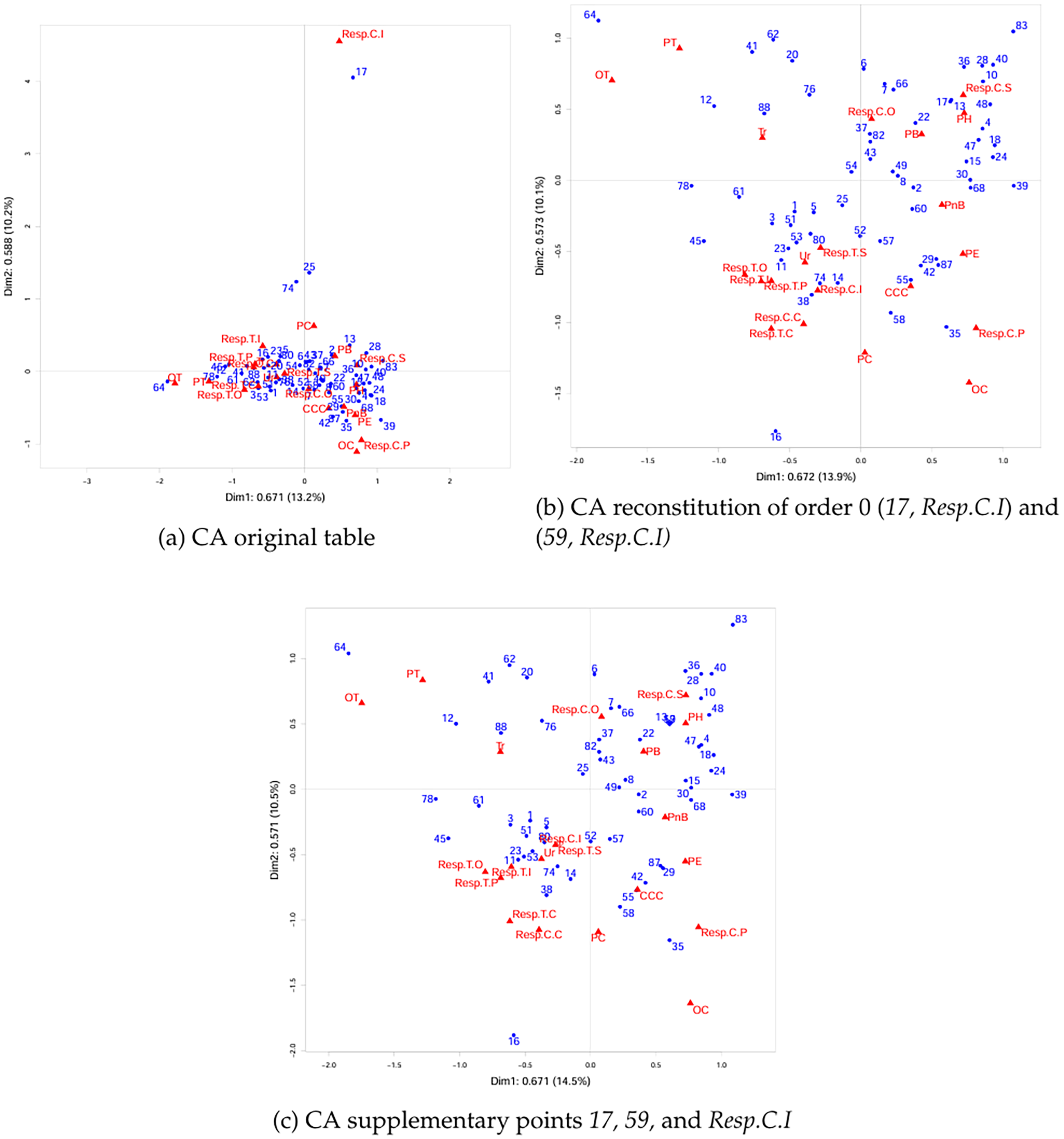
CA plot about Ocean plastic dataset

The first dimension contrasts Opportunity due to treatment (OT), Treatment related problems (PT) and Treatment recommendation (Tr), Responsibility for treatment framings T.O, T.P, T.C and T.I on the left versus responsibility for causes framings C.P, C.S and C.I, and Problem definitions such as Opportunity (OC), Health (PH), Economic (PE), Non-Biological (PnB), and Biological (PB) on the right. On the second dimension, Resp.C.I, i.e. industry is responsible for cause, is far from the origin. The marginal proportion of Resp.C.I is 0.013, and its contribution to the second dimension is 76.9%. Resp.C.I masks the visualisation of the structure in the dataset and reduces the readability of this map. Documents 17, 59, which have identical scores, are far from the origin and are closest to Resp.C.I. The marginal proportion of documents 17/59 jointly is 0.013, yet its contribution to the second dimension is 61.0%. Also, the contribution of the two cells (17/59, Resp.C.I) to the total inertia is 7.0%, which is large (note that there are 81 × 21 cells). Hence the cells (17/59, Resp.C.I) are cell-wise outliers, leading to outlying points for 17, 59 and Resp.C.I on dimension 2.

Reconstitution algorithm

Again, we used the reconstitution algorithm of order 2 to handle the cell-wise outliers. However, this created a negative imputed value −0.0006 for outlying cells (17/59, Resp.C.I). Negative values are not easy to interpret in an incidence matrix. Therefore, we applied reconstitution of order 0. This yields value 0.0065 for the cells (17/59, Resp.C.I). Now the documents 17/59, having a 1 in the framing variable PB, 0.0065 in Resp.C.I and otherwise 0, are similar to documents 13, 19, 26, 27, 46, 56, 65, 69, 84 which have 1 in PB and 0 otherwise. The first four singular values are 0.672 (13.9%), 0.573 (10.1%), 0.548 (9.3%), and 0.519 (8.3%).

Figure 7b is a symmetric CA plot of the reconstituted table. On the first dimension the configuration of column points is similar to the configuration in Figure 7a, except for Resp.C.I. Resp.C.I is not close to Documents 17/59, and Resp.C.I, 17/59 are not far from the origin. Now, the contributions to the second dimension of Resp.C.I is only 1.2% and of 17/59 jointly 0.6%.

By reducing the influence of cells (17/59, Resp.C.I), the new figure is much better readable than Figure 7a. A full interpretation of the table makes use of the outliers found in standard CA, and the CA solution found with the reconstitution method. The standard CA reveals a strong positive relation between 17/59 and Resp.C.I. We interpret the CA solution found with the reconstitution method by interpreting the four quadrants of Figure 7b.

Press releases in the first quadrant focus on problems related to biology (PB) and human health (PH), and place the responsibility for causes at society (Resp.C.S);

The second quadrant represents problems related to treatment (PT) and solutions to these problems in the form of treatment (Tr), and opportunity if treatment is carried out (OT);

Press releases in the third quadrant focus on the urgency to treat ocean plastic (Ur) and hold entity responsible for carrying out that treatment (Resp.T.C, Resp.T.P, Resp.T.I, Resp.T.O, Resp.T.S). In some cases they also state the responsibility for cause at industry (Resp.C.I) and specific regions/countries (Resp.C.C);

Press releases in the fourth quadrant focus on the interconnections between ocean plastic and climate change (CCC) and they state non-biological (PnB) and economic consequences (PE). The fourth quadrant also represents the responsibility for cause at politics (Resp.C.P) and opportunity due to problems (OC). We note that the marginal frequencies of Resp.C.P and OC are low, namely 1 and 2 respectively.

Supplementary points method

Here we treat 17/59 and Resp.C.I as supplementary points. Thus the size of the table analysed is 79x 20. Now, due to deleting Resp.C.I, documents 25 and 54 are also identical. Rows 17/59 and column Resp.C.I have no effect on the solution of CA but are projected into it afterwards. The first four singular values are 0.671 (14.5%), 0.571 (10.5%), 0.544 (9.6%), and 0.511 (8.4%).

Figure 7c shows the symmetric CA plot for the supplementary points method. Figure 7c is similar to Figure 7b.

Discussion and conclusion

In this paper, we propose to use the reconstitution algorithm of order h to deal with outlying cells in CA. The reconstitution algorithm of order h can reduce the effects of single outlying cells on the CA solution. We compare it with MacroPCA and the supplementary points method.

In comparison to the reconstitution approach, MacroPCA imputes outlying cells in the matrix of standardized residuals instead of in the original matrix. Apart from imputing cell-wise outliers, it can also eliminate complete rows. Yet, MacroPCA is not as transparent and straightforward as the reconstitution approach. One of the reasons is that it is originally proposed for the analysis continuous data and makes distributional assumptions, which do not hold for the reconstitution approach. Due to these distributional assumptions, that do not always fit with how the data originate, in our view it appears to flag too many cells as outlying cells.

The supplementary points method deletes complete rows or columns. In contrast, the reconstitution algorithm only reduces the influence of outlying cells. Thus, the reconstitution algorithm uses more information in the data and is, from this perspective, preferable.

To compare the three methods, we simulated datasets with known properties. We simulated three scenarios: a contingency table with CA dimensionality 0, 1, and 2, each with and without an outlying cell. The experimental results showed that, for these created datasets, reconstitution of order h was able to reproduce the underlying dimensionality structure if the dimensionality h was used with which the table was created. Overall, the supplementary point method also works fine, but it ignores more information than necessary. The MacroPCA does not work well in the simulated data that we created.

We analysed two real data sets to illustrate the use of the reconstitution algorithm and compared the algorithm with the supplementary points method and MacroPCA. For the contingency table car dataset, the three methods yielded similar results. For the ocean plastic dataset, the reconstitution algorithm and the supplementary points method had similar results, but MacroPCA failed.

We are not able to show empirically that the reconstitution method is preferable over the supplementary points method and MacroPCA. However, on theoretical grounds the reconstitution method is preferable: it eliminates only single cells to handle outlier problems, thus it is not necessarily deleting more information than is necessary.

In this paper, to detect cell-wise outliers, we follow Greenacre’s definition using visual inspection of the CA plot. We recognize that it is important to also further develop quantitative approaches to identify outliers in the context of reconstitution of order h (Hawkins, 1980; Riani et al., 2022; Rousseeuw & Hubert, 2011). This is particularly true in this area of big data and data science. We leave this topic for future studies. Likewise, there is also a lack of objective evaluation of the information gain from the reconstitution algorithm, as well as the biases associated with the presented method. We also leave this topic for future studies.

In this paper, we compare reconstitution algorithm with MacroPCA and supplementary points method which are used before to deal with outliers in CA (Greenacre, 2017; Raymaekers & Rousseeuw, 2024; Riani et al., 2022). There are other robust methods about robust CA, such as taxicab CA (Choulakian, 2006b, 2020) or the contribution biplot (Greenacre, 2013). Taxicab CA uses L1 optimization and gives uniform weights to all points. The contribution biplot represents rows or columns by their contribution to axis and thus reduces the influence of row or column margins on the CA plot. Further, robust PCA methods, including L1-norm PCA (Choulakian, 2006a), ROBPCA-AO (Hubert et al., 2009), and PP-PCA (Croux et al., 2007), can be adapted to CA and be used to compare with the reconstitution algorithm. These comparisons are also left for future studies.

Last, we focus on CA with two categorical variables. An extension of CA designed for categorical data with more than two variables is multiple CA (Le Roux & Rouanet, 2010). The application of the reconstitution algorithm to multiple CA is also a study area of interest.

Software

The reconstitution algorithm of order h is implemented by a function reconca both for $h = 0$ and $h > 0$ . The function is written by adjusting the function imputeCA in the R Package missMDA. Josse and Husson (2016) proposed the R package missMDA for handling missing values in multivariate data analysis, where the function imputeCA is meant for missing values in CA. Another R Package, which can perform a reconstitution algorithm of order zero, is anacor, proposed for simple and canonical CA by De Leeuw and Mair (2009), to deal with missing data in CA.

The MacroPCA method is performed by the MacroPCA function in R package cellWise. The MacroPCA method is proposed for PCA (Hubert et al., 2019) and adjusted for CA (Raymaekers & Rousseeuw, 2024). To fit CA, the original matrix is replaced with the matrix of standardized residuals.

The code to reproduce the results of this paper is on the GitHub website https://github.com/qianqianqi28/CA-outlier-reconstitution-algorithm/. Specifically, the function reconca is in https://github.com/qianqianqi28/CA-outlier-reconstitution-algorithm/tree/main/R.

Supplemental Material

sj-pdf-1-bms-10.1177_07591063251348789 - Supplemental material for Correspondence analysis: Handling cell-wise outliers via the reconstitution algorithm

Supplemental material, sj-pdf-1-bms-10.1177_07591063251348789 for Correspondence analysis: Handling cell-wise outliers via the reconstitution algorithm by Qianqian Qi, David J. Hessen, Aike N. Vonk and Peter G. M. van der Heijden in Bulletin of Sociological Methodology/Bulletin de Méthodologie Sociologique

Footnotes

Declaration of conflicting interests

The authors declared no potential conflicts of interest with respect to the research, authorship, and/or publication of this article.

Déclaration de conflits d'intérêts

Les auteurs ont déclaré n'avoir aucun conflit d'intérêt potentiel pour tout ce qui concerne le déroulement de la recherche, les droits d'auteur et/ou la publication de cet article.

Funding

The authors disclosed receipt of the following financial support for the research, authorship, and/or publication of this article: Qianqian Qi is supported by the China Scholarship Council (CSC202007720017).

Financement

Les auteurs déclarent que Qianqian Qi bénéficie du soutien du China Scholarship Council (CSC202007720017).

Matériel supplémentaire

Des documents supplémentaires sont disponibles en ligne

Supplemental material

Supplemental material for this article is available online.

References

Andersen

Mayerl

(2017) Social desirability and undesirability effects on survey response latencies. Bulletin of Sociological Methodology/Bulletin de Méthodologie Sociologique 135(1): 6889.

Bendixen

(1996) A practical guide to the use of correspondence analysis in marketing research. Marketing Research On-Line.

Choulakian

(2006a) L1-norm projection pursuit principal component analysis. Computational Statistics & Data Analysis 50(6): 1441-1451.

Choulakian

(2006b) Taxicab correspondence analysis. Psychometrika, 71(2), 333-345.

Choulakian

(2020) Taxicab correspondence analysis of sparse two-way contingency tables. Statistica Applicata - Italian Journal of Applied Statistics 29(2-3): 153-179.

Croux

Filzmoser

Oliveira M

(2007) Algorithms for projection–pursuit robust principal component analysis. Chemometrics and Intelligent Laboratory Systems 87(2): 218-225.

De Leeuw

Mair

(2009) Simple and canonical correspondence analysis using the R package anacor. Journal of Statistical Software 31(5): 1-18.

De Leeuw

Van der Heijden

PGM

(1988) Correspondence analysis of incomplete contingency tables. Psychometrika 53(2): 223-233.

De Leeuw

Van der Heijden

PGM

Verboon

(1990) A latent time–budget model. Statistica Neerlandica 44(1): 1-22.

10.

Entman

(1993) Framing: Toward clarification of a fractured paradigm. Journal of Communication 43(4): 51-58.

11.

Gabriel

(1971) The biplot graphic display of matrices with application to principal component analysis. Biometrika 58(3): 453-467.

12.

Gower

Hand

(1996) Biplots. Chapman & Hall.

13.

Greenacre

(1984) Theory and Applications of Correspondence Analysis. London: Academic Press.

14.

Greenacre

(2013). The contributions of rare objects in correspondence analysis. Ecology 94(1): 241-249.

15.

Greenacre

(2017). Correspondence Analysis in Practice. CRC press.

16.

Greenacre

(2018). Compositional Data Analysis in Practice. Chapman and Hall/CRC.

17.

Greenacre

Hastie

(1987) The geometric interpretation of correspondence analysis. Journal of the American Statistical Association 82(398): 437-447.

18.

Grubbs

(1969) Procedures for detecting outlying observations in samples. Technometrics 11(1), 1-21.

19.

Hawkins

(1980) Identification of outliers. Springer.

20.

Hoffman

Franke

(1986) Correspondence analysis: Graphical representation of categorical data in marketing research. Journal of Marketing Research 23(3): 213-227.

21.

Hubert

Rousseeuw

Verdonck

(2009) Robust PCA for skewed data and its outlier map. Computational Statistics & Data Analysis 53(6): 2264-2274.

22.

Hubert

Rousseeuw

Van den Bossche

(2019) MacroPCA: An all-in-one PCA method allowing for missing values as well as cellwise and rowwise outliers. Technometrics 61(4): 459-473.

23.

Josse

Chavent

Liquet

Husson

(2012) Handling missing values with regularized iterative multiple correspondence analysis. Journal of Classification 29: 91-116.

24.

Josse

Husson

(2016) missMDA: A package for handling missing values in multivariate data analysis. Journal of Statistical Software 70(1): 1-31.

25.

Kienstra

Van der Heijden

PGM

(2015) Using correspondence analysis in multiple case studies. Bulletin of Sociological Methodology/Bulletin de Méthodologie Sociologique 128(1): 5-22.

26.

Kim

S-K

McKay

Murphy T

Bussing

McNamara J

Goodman W

Storch E

(2021) Age moderated–anxiety mediation for multimodal treatment outcome among children with obsessive-compulsive disorder: An evaluation with correspondence analysis. Journal of Affective Disorders 282: 766-775.

27.

Kuhnt

Rapallo

Rehage

(2014) Outlier detection in contingency tables based on minimal patterns. Statistics and Computing 24: 481-491.

28.

Le Roux

Rouanet

(2010) Multiple Correspondence Analysis. Thousand Oaks, CA : Sage.

29.

Nora-Chouteau

(1974) Une méthode de reconstitution et d’analyse de données incomplètes. Unpublished doctoral dissertation. Université Pierre et Marie Curie, Paris, France.

30.

Pitt

Bal

Plangger

(2020) New approaches to psychographic consumer segmentation: Exploring fine art collectors using artificial intelligence, automated text analysis and correspondence analysis. European Journal of Marketing 54(2): 305-326.

31.

Hessen

Deoskar

Van der Heijden

PGM

(2024) A comparison of latent semantic analysis and correspondence analysis of document-term matrices. Natural Language Engineering 30(4): 722-752

32.

Raymaekers

Rousseeuw

(2024) Challenges of cellwise outliers. Econometrics and Statistics. DOI: https://doi.org/10.1016/j.ecosta.2024.02.002

33.

Raymaekers

Rousseeuw

Van den Bossche

Hubert

(2023) CellWise: Analyzing Data with Cellwise Outliers . R package version 2.5.3.

34.

Riani M

Atkinson

Torti F

Corbellini

(2022) Robust correspondence analysis. Journal of the Royal Statistical Society Series C: Applied Statistics 71(5): 1381-1401.

35.

Robette

(2022) Trees and forest. Recursive partitioning as an alternative to parametric regression models in social sciences. Bulletin of Sociological Methodology/Bulletin de Méthodologie Sociologique 156(1): 7-56.

36.

Rousseeuw

Hubert

(2011) Robust statistics for outlier detection. Wiley Interdisciplinary Reviews: Data Mining and Knowledge Discovery 1(1): 73-79.

37.

Rousseeuw

Van Den Bossche

(2018) Detecting deviating data cells. Technometrics, 60(2): 135-145.

38.

Sripriya

Srinivasan

(2018) Detection of outlying cells in two-way contingency tables. Statistics and Applications 16(2): 103-113.

39.

Vonk

Bos

Smeets

Van Sebille

(2024) A comparative study of frames and narratives identified within scientific press releases on ocean climate change and ocean plastic. Journal of Science Communication 23(1): A01.

Supplementary Material

Please find the following supplemental material available below.

For Open Access articles published under a Creative Commons License, all supplemental material carries the same license as the article it is associated with.

For non-Open Access articles published, all supplemental material carries a non-exclusive license, and permission requests for re-use of supplemental material or any part of supplemental material shall be sent directly to the copyright owner as specified in the copyright notice associated with the article.

0.00 MB

1.51 MB