
Abstract
Due to Covid-19 restrictions, surveys often could not be conducted in originally planned face-to-face mode, and switched to online modes or used different mixed-mode designs. A combination of CATI and CAPI was used for the Austrian ISSP survey on Environment 2020/2021 (N=1.261), which in the past had always been conducted face-to-face. Mixed-mode surveys facilitate field access in pandemic times and show potential to reduce non-response and coverage errors (desired selection effect). However, the combination of different modes comes along with a series of risks such as mode-effects causing bias due to measurement effects. From an analytical perspective, the challenge arising is to disentangle selection and measurement effects. Thus, we analyse differences in the factorial structure and response distributions of two social constructs using Bayesian multigroup confirmatory factor analysis and linear regression. These represent institutional trust and the willingness to sacrifice for environmental protection. The findings show support for scalar invariance and therefore the absence of CAPI vs. CATI mode-effects on the factorial structure for both constructs. However, despite adjusting for differences in sample composition we observe a higher average willingness within the CATI sample. Based on these results, we discuss implications for the interpretation of mode effects in mixed mode surveys.
Introduction
Due to far-reaching contact restrictions and to minimise the risk of infection for interviewees in the wake of the Covid-19 pandemic, imposed by governments of many countries, several surveys could not be conducted in their original face-to-face mode. Thus, some surveys used self-administered paper questionnaires delivered and collected by mail, while others switched to self- or interviewer-administered (video-based) online-modes (for a general overview see Vehovar and Manfreda, 2017), including push-to-web approaches (Dillman, 2017; Lynn, 2020), or used different mixed-mode designs (e.g. Bosnjak, 2017; Leitgöb, 2017; de Leeuw et al., 2018).
The cross-country comparative surveys of the International Social Survey Programme (ISSP 1 ) – in many countries – are still conducted face-to-face and therefore, were affected by severe problems realising the planned fieldwork in 2020 and 2021 (for mixed modes in international comparative surveys see de Leeuw et al., 2018). This was also the case for the Austrian representative population survey of the ISSP-Module on “Environment”. In Austria, ISSP surveys had always been conducted in face-to-face interviews since the 1980s. However, in spring 2021, after postponing the fieldwork of the Austrian ISSP twice, the decision has been made to use a mixed-mode design combining CATI (Computer Assisted Telephone Interviews) and CAPI (Computer Assisted Personal Interviews). In contrast to mixed-mode designs, in which cost-effective self-administered modes are combined with a costly interviewer-administered mode (Blom et al., 2016; Bosnjak, 2017), CATI and CAPI are both interviewer-administered and, in the Austrian case, were not selected for the reasons of cost, but because CAPI could not be carried out in times of lockdowns. 2 Therefore, the fieldwork began with CATI and, once the Corona situation had calmed down, only CAPI were conducted. In this mixed-mode design, respondents did not have the opportunity to choose between CATI and CAPI.
Given this change in survey mode, the question of potential mode effects arises, i.e. whether the different modes of data collection led to differences in measurement structure as well as to differences in response patterns. Mode effects must be understood as net effects of “non-observation and measurement error differences between the modes” (de Leeuw, 2018: 79). Despite the known advantages of mixed-mode designs, such as the reduction of coverage errors and non-response (e.g., de Leeuw, 2018; Tourangeau, 2017), “mode effects can make MM [mixed mode] data highly unusable by simultaneously generating selection effects and measurement effects (measurement error)” (Vannieuwenhuyze et al., 2010: 1028). Measurement effects can affect both, the response distribution as well as the measurement structure of latent variables (Hox et al., 2015). Against this backdrop, this paper follows the claim to investigate mode effects by analysing selection and measurement effects (Vannieuwenhuyze et al., 2010; Vannieuwenhuyze, 2013).
We therefore analyse the response distributions and factor structure 3 of two widely used social constructs: (1.) people’s trust in societal institutions (referred to as ‘institutional trust’) and (2.) people’s willingness to pay higher taxes, higher prices, and to cut the own standard of living for environmental protection (referred to as ‘willingness to sacrifice for the environment’), which are both part of the ISSP-Module on “Environment”. The question wording on these two social constructs was identical in both modes. We use Bayesian Multigroup Confirmatory Factor Analysis and linear regression instead of frequentist approaches because it offers a higher utility in extracting mode-effects as well as reporting results by detailed information of posterior distributions. Our research questions are as follows: Which sociodemographic groups of respondents are attracted by the different survey modes of CATI and CAPI (selection effects)? To what extent do these different modes affect response patterns to questions about ‘institutional trust’ and ‘willingness to sacrifice’ for the environment (measurement effects)?
Our findings show support for scalar invariance and therefore the absence of mode-effects on the factor structure for both social constructs. We though find small differences in the response distributions between both modes for the ‘willingness to sacrifice for the environment’. These differences decrease when adjusting for socio-demographics and are partly due to distinctions in sample composition. Based on these results, we will highlight explanations and further implications for future analysis and interpretation of mixed-mode effects.
In the next section, we provide basic information towards the reasons for and consequences of the combination of different survey modes, and discuss the important distinction between desired selection effects and unwanted measurement effects. This section is followed by a presentation of the data and methods used for the analyses of selection and measurement effects. Subsequently, we first compare descriptive findings of the CAPI and CATI sample; second, we present results on the equivalence of measurements by means of Multi-Group Factor Analyses; and third, we test for mode differences using Bayesian linear regression models. The conclusion ties together our findings and discussions on analysing and evaluating mode effects.
Desired selection effects and unwanted measurement effects
Despite the various possibilities to combine different modes of data collection in survey research, face-to-face interviews are still considered among the most reliable modes of data collection by many survey programmes. The main reasons for this lie in the improved quality control as interviewers visit the respondents in person making it possible to verify who in fact answers the survey questions and review question comprehension in response behaviour. However, due to high costs of the face-to-face mode, severe and increasing coverage and non-response errors (de Leeuw et al., 2008; de Leeuw and de Heer, 2002) interviewer effects as well as technological enhancements in the field of self-administered digital modes mixed-mode designs have gained growing importance (de Leeuw, 2018).
Mixed-mode surveys facilitate field access and show great potential to reduce non-response and coverage errors. Survey researchers particularly hope to better reach respondents of different age, level of education, technology affinity, levels of literacy etc. and of different motivations to participate in surveys by offering varying survey modes. “From a Total Survey Error perspective, one wants the best of all worlds and aims to reduce overall error” (de Leeuw, 2018: 80). In order to reduce costs of surveys a typical mix of modes considers the combination of smaller samples of high-cost survey modes in combination with larger samples of low-cost survey modes (Blom et al., 2016; Bosnjak, 2017).
However, the combination of different survey modes comes along with a series of risks such as mode-effects causing bias due to measurement effects. This raises the question if the specific errors of the individual survey modes might even accumulate (de Leeuw, 2018; de Leeuw, 2005) respectively cause new unwanted biases. Thus, the goal of using mixed modes lies in the reduction of coverage and non-response errors by using the selection effects of the different modes (desired selection effect), and to simultaneously avoid measurement effects which lead to differentiated error structures and biased estimates (unwanted measurement effects) (de Leeuw, 2018; Vannieuwenhuyze et al., 2014). Moreover, measurement effects leading to shifts in mean values need to be further examined to see whether they also influence correlations (Hox et al., 2017).
The methods for testing mode effects have been greatly developed in the last few years. Typical challenges consider to adequately disentangle selection and measurement effects and to investigate the causal influence of different modes on responses (Leitgöb, 2017). Since selection and measurement effects are confounded, “[D]differences (or similarities) between the outcomes of modes can be caused by differences between the respondents or by differences in measurement error” (Vannieuwenhuyze et al., 2010: 1028). Ultimately, researchers cannot be sure if respondents had answered survey questions differently under a different mode.
A typical way to investigate selection effects is to compare response rates as well as the sociodemographic groups reached by each survey mode by means of sociodemographic variables such as age, gender, education, etc. From the literature it can be assumed that response rates are higher for CAPI than for other modes (Vannieuwenhuyze et al., 2010). If samples are drawn from the same sampling frame, the comparison of socio-demographics of the different survey modes, on the one hand, should not be statistically significantly different, if there are no mode selection effects (Vannieuwenhuyze et al., 2010). On the other hand, different modes are intended to better reach certain population groups. Cornesse and Bosnjak (2018) found that mixing modes in some surveys positively contributes to the representativeness in surveys referred to sociodemographic characteristics of respondents. However, these desired selection effects with regard to sociodemographic characteristics do not guarantee a balanced distribution of attitudes, values or other target variables.
Mode-effects are typically analysed by estimating the impact of the modes on selected outcome variables such as attitudinal scales. Different kinds of regression models are used to test the effect of the mode on the outcome variable and control for sociodemographics and other important impact factors known from the literature. However, “demographic variables are generally not strong predictors of selection into different modes, and therefore this procedure tends to underestimate the selection bias, and hence overestimate and overadjust the measurement bias” (Hox et al., 2017: 513). To validate the measurement structure across modes, invariance tests using Multi-Group Factor Analysis are recommended (Hox et al., 2015).
Previous research on mode-effects shows a mixed picture of results depending on the specific mixed-mode design, the methods used to analyse the mode effects, and the selected social constructs used for the analysis (e.g., Hox et al., 2017). Moreover, differences in response patterns have been interpreted differently regarding its causes and consequences and the question if these indicate substantial mode-effects. Overall, Hox et al. (2017) conclude from several studies that measurement effects are typically small and become even smaller when they are controlled for sociodemographics and other relevant factors. Comparisons of telephone and face-to-face interviews generally show little differences in terms of response patterns, measurement structure and social desirability; they are smaller compared to the differences between self-administered and interviewer-administered modes (de Leeuw, 2018). Apart from the communalities between CATI and CAPI, complex questions that benefit from a visual presentation are problematic to field via CATI (Groves, 1979; 1990), especially if no showcards are sent to respondents before the interview. Even if showcards are included in the CATI design, respondents are responsible for selecting the right showcard themselves and only get explanations on the phone.
Data and methods
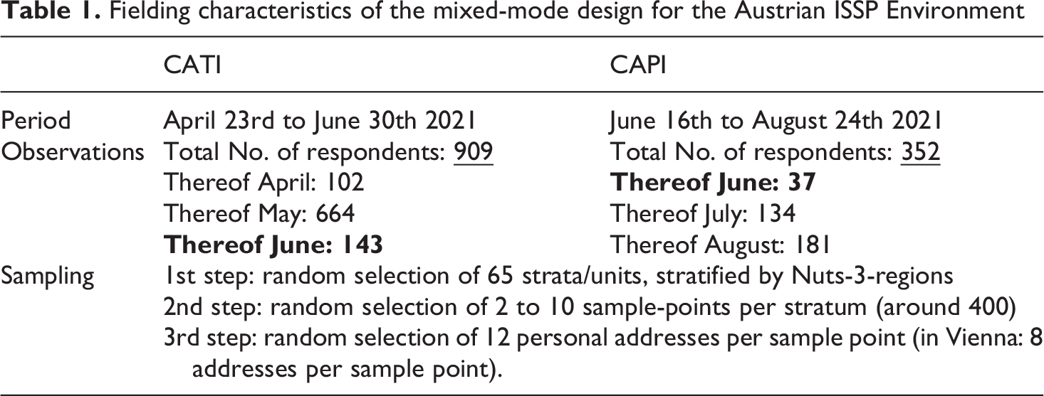
The analyses in this paper are based on data from the representative population survey of the Austrian ISSP Module on Environment in which 1.261 respondents, aged 18 and above, were interviewed by either CATI or CAPI between April and August 2021 (Hadler et al., 2022). As already mentioned in the introduction, CATI and CAPI were fielded after another, where CATI was the predefined mode from April to June 2021, when Austria still imposed lockdowns due to the Covid-19 pandemic. CAPI were conducted from June 2021 onwards, with both CATI and CAPI being conducted for a short period in June (see Table 1). Thus, respondents could not choose between CATI and CAPI and the short overlapping period of both modes was only due to the completion of already agreed interview appointments.
Fielding characteristics of the mixed-mode design for the Austrian ISSP Environment
Pretests of the questionnaire were carried out both by telephone and face-to-face in order to test the functionality of the modes, the comprehensibility of the questions and wording, completeness of the items and scales, length of the survey, and filter guides, as well as to compare these criteria between modes. On the basis of these pretests, some adaptions were made (mainly interviewer instructions), however, the questions themselves could not be changed because they were voted on in the international committee of the ISSP. In addition, the decision was made to send CATI-respondents selected showcards together with the invitation letter of the survey in order to give a visual stimulus for answering the most complex questions of the module. However, with regard to the questions analysed in this paper only three items measuring the willingness to sacrifice for the environment were fielded using showcards but only in the CAPI mode. In general, showcards were used more often in the CAPI than in the CATI mode.
The sample was drawn on the basis of multistage random sampling (based on NUTS-3-regions), with the sampling frame comprising recent address data from Austrian Post (addresses of private households). This almost completely covers the Austrian resident population with a low non-coverage bias. The calculation of the necessary sample points was based on the assumption that up to six interviews can be achieved on a given address list of twelve addresses. In Vienna (the only large city in Austria), more lists are generally provided, but only with eight addresses in order to minimise clumping in urban areas. In the other federal states, lists with twelve addresses were specified, as the spatial distances would otherwise be too great. The allocation of sample points to the strata was based on current population data from the statistical office “Statistics Austria”. One or more sample points are required per stratum, within which a random selection of counting clusters (clumps) is made. The first counting clump is selected at random. If several counting clusters are required per stratum (usually in cities), every xth cluster is drawn according to a key number. The population size is taken into account when drawing the counting districts so that the selection probabilities are not distorted. The required number of addresses is then drawn at random for each clump. The final utilisation rate was 25-30%. 4 Table 1 gives an overview of the number of respondents of each mode, the temporal sequence of fielding and the sampling procedure of multistage random sampling on the basis of respondents’ addresses.
Given that visits to homes were not allowed during the early stage of the fieldwork, interviewers were asked to look up the 12 names (8 names in Vienna) in the public phone directory and to call the individuals that were listed. In the course of the pandemic-related methodological changeover of the survey to CATI, the address lists were expanded to take account of the fact that only half of the addresses can be enriched with telephone numbers from publicly accessible telephone directories. The gross sample with telephone numbers amounted to around 2,300 addresses. In the later stage of the fieldwork, visits to houses were allowed again and interviewees were conducted face-to-face only. During this CAPI stage especially households of the original sample but without a telephone number were contacted for interviews.
The target households were informed by a notification letter with information on the study, data protection and information on an upcoming call or visit by the interviewer (including a telephone hotline for queries). In the case of CAPI, reference was also made to the strict Covid-19 safety precautions during the interview. However, at the beginning of the CAPI field period infection numbers were low, the majority of governmental restrictions were loosened or temporarily repealed, and the fear of the virus in the general public decreased (for an overview of survey research in times of Austrian pandemic management see Eder et al., forthcoming 2024).
In this paper, we select two social constructs from the ISSP-Environment Module which are well established in several large-scale survey programmes and thus of particular interest for researchers (see Figure 1). People’s willingness to pay higher taxes, higher prices, and to cut the own standard of living for environmental protection considers the first social construct; people’s trust in societal institutions like universities or the parliament considers the second construct. Response categories for the willingness to sacrifice for the environment consisted of a five-point scale reaching from “very acceptable” to “very unacceptable” and were recoded for the analyses so that higher values represent higher acceptance. Institutional trust was measured on a 10-point scale with higher values indicating greater trust. As both modes are interviewer-administered, there is little reason to assume substantial differences in responses between modes. However, it is unclear how lockdown situations and potential fears of face-to-face contact affect interview participation and mode preferences for interviews.
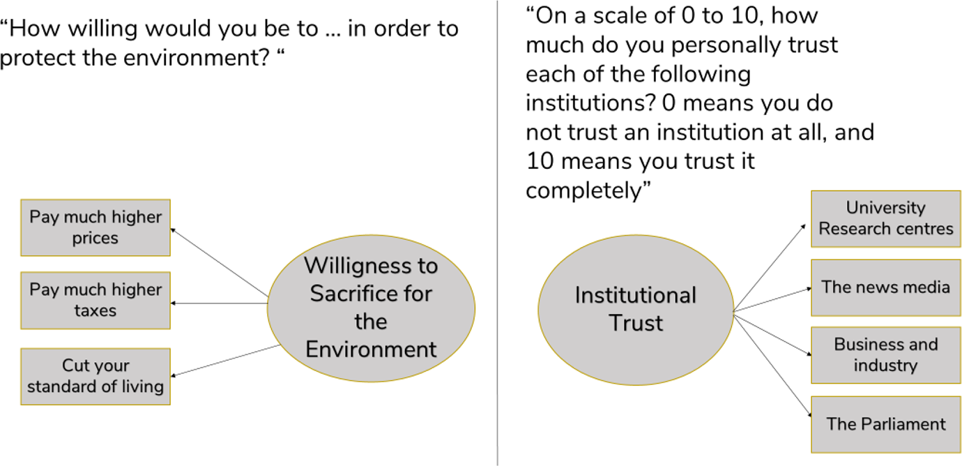
Survey questions of the social constructs of the analyses
Our analysis proceeds in three steps. The first step is to identify selection effects by providing descriptive statistics of the sample and testing for differences in the CATI-CAPI sample composition. In the remaining two steps, we focus on unwanted measurement effects in the response distributions as well as the factor structures of both social constructs for which we use a Bayesian approach. This approach differs from classical Frequentist methods not only in its estimation technique but also in its understanding of probability. The probability from a posterior distribution describes the uncertainty about a parameter, taking into account prior information (“prior”) and the statistical results of our model (“likelihood”) (Kruschke, 2015). In contrast to classical statistics, we can therefore place probability statements around parameters using so-called credible intervals. These should not be confused with classical confidence intervals as they are interpreted differently. We report our estimates with 95% credible intervals, which can be understood as the parameter having a 95% probability of falling within this interval, given our observed data (McElreath, 2016). As we will show in the results section, this allows for a more transparent way of communicating the differences between modes and, in particular, the uncertainty associated with them. Complex posterior distribution cannot be solved analytically therefore, Markov Chain Monte Carlo (MCMC) simulations are used to draw samples from a posterior. We use R-packages which are built on the probabilistic language Stan (Carpenter et al., 2017). Stan uses a no-turn MCMC technique to draw samples from a posterior distribution (for a reader friendly introduction to this technique, see Betancourt (2017)). Following Lemoine (2019), we use weakly informative prior distributions for all model parameters.
In the first step, we show the distributions of central sociodemographic data (gender, age, education, income) as well as of political background variables (political party preference, political interest, and left-right self-assessment) in the two modes in order to analyse similarities and differences in the sample composition. The goal of this comparison is to identify selection effects.
In the second step, we assess survey-mode related differences in the measurement of both social constructs. Following Hox et al. (2015), we use Multi Group Confirmatory Factor Analysis (MGCFA) to test for measurement invariance. MGCFAs were estimated in a Bayesian framework using the R-package blavaan (Merkle and Rosseel, 2018). As recommend in the literature, we test three consecutive forms of invariance: configural invariance, metric invariance, and scalar invariance (Steenkamp and Baumgartner, 1998; van de Schoot et al., 2012; Vandenberg and Lance, 2000). First, we test for configural invariance in order to test if we measure the same factors in both groups (modes) (Vandenberg and Lance, 2000). We continue with metric invariance by testing whether factor loadings are equal across both modes. Finally, we constrain item-intercepts to be equal in order to test for scalar invariance (Steenkamp and Baumgartner, 1998).
In the literature, it is strongly recommended to evaluate several fit indices when assessing measurement invariance (Klausch et al., 2013; van de Schoot et al., 2012). Therefore, we use three metrics for our invariance tests: the Leave-One-Out Cross-Validation Information Criterion (LOOIC), Bayesian Root Mean Square Error of Approximation (BRSMEA) and Bayesian Comparative Fit Index (BCFI). LOOIC is an information criterion which takes into account both, fit as well as model complexity. Despite mathematical differences, its interpretation is the same as for other information criteria such as AIC and BIC which implies that absolute values must be compared across models with decreasing values indicating a better balance of model complexity and fit (Vehtari et al., 2017). BRSMEA is the Bayesian counterpart to RMSEA and BCFI to CFI. BRSMEA is a badness of fit index with low values pointing to a good fit while BCFI indicates the incremental growth explanatory power compared to a null model (Garnier-Villarreal and Jorgensen, 2020). As recommended by Garnier-Villarreal and Jorgensen (2020), we use established thresholds to evaluate the invariance across both modes. Therefore BRSMEA ≤ 0.05 and BCFI ≥ 0.90 indicate a good fit. We additionally present both indices with a 95% credible interval to quantify uncertainty around their point estimates.
In the third step, we use Bayesian linear models and regress average scores of both scales on our survey-mode variable. Finally, we adjust mode-differences for socio-demographics 5 . Linear regression models are estimated using the R-package rstanarm (Goodrich et al., 2022), again assuming weakly informative priors for all model parameters.
Results
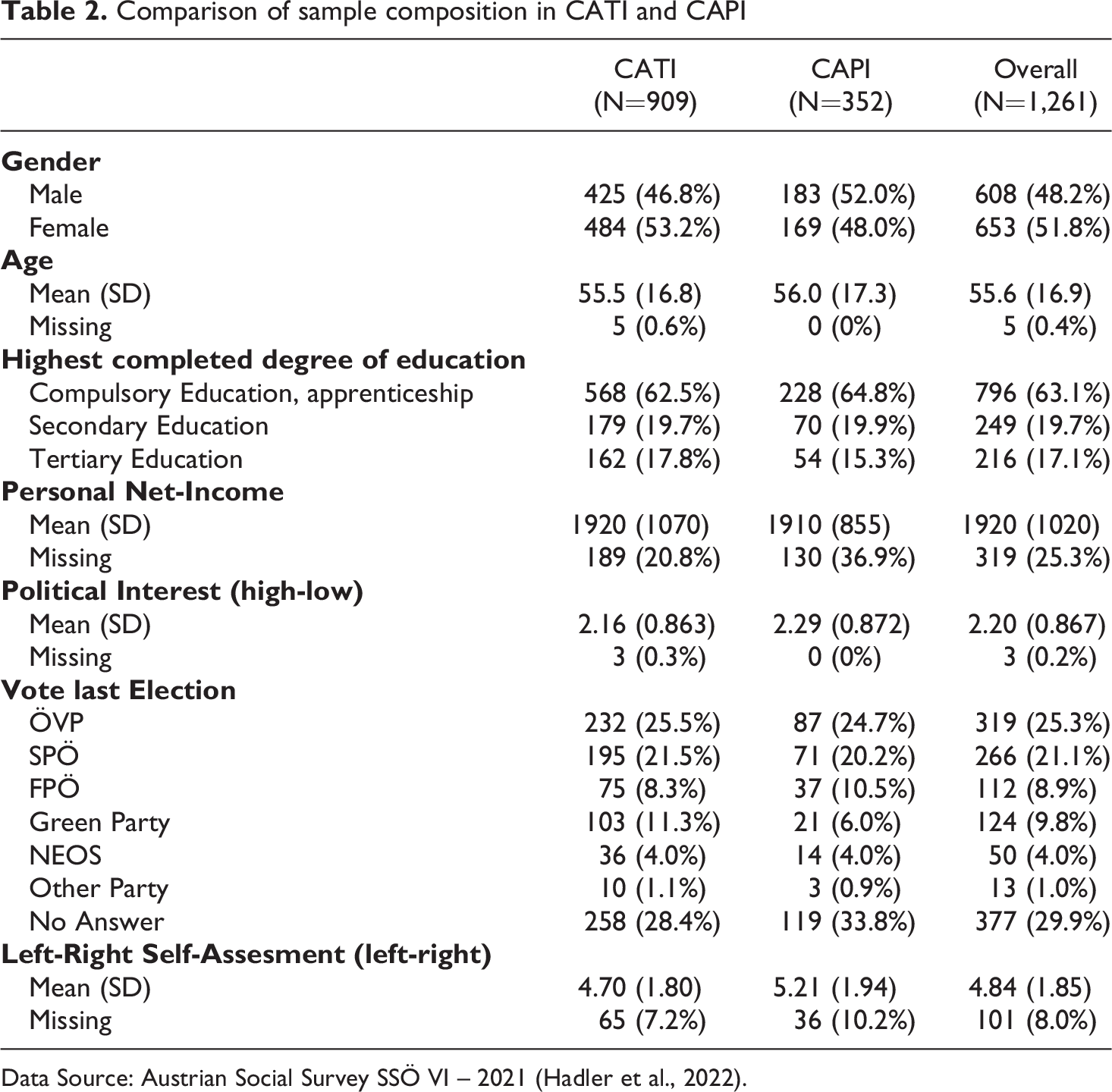
Table 2 shows a comparison of the distributions of central sociodemographic data and political background variables in the two modes (CATI and CAPI). Results of chi-square and t-tests suggest no pronounced and statistically non-significant differences for age, education, political interest, and income. We find a higher, but non-significant (p = .108; χ2 = 2.578) proportion of men in the CAPI sample and a tendency towards right-wing political orientation which is reflected in a higher proportion of voters for Austria’s right-wing party FPÖ (CATI: 8.3% vs. CAPI: 10.5%) and lower proportion of left-wing voters of the Greens (CATI: 11.3% vs. CAPI: 6.0%). This results in a significant difference between CATI and CAPI in terms of voting preferences (p < .05, χ2 = 11.34). Furthermore, we see a statistically significant higher mean (p < 0.001; t = −4.002) indicating a stronger presence of politically right-wing oriented respondents in the CAPI-mode (CATImean = 4.70; CAPImean = 5.21). We will consider these disparities in the sample composition in our statistical models below.
Comparison of sample composition in CATI and CAPI
Data Source: Austrian Social Survey SSÖ VI – 2021 (Hadler et al., 2022).
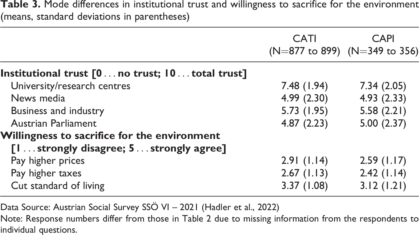
Regarding potential mode differences in the response behaviour of our two central social constructs (see Table 3), the comparison of means suggests only small differences. Nevertheless, CATI-respondents are consistently more willing to get engaged for the environment than CAPI-respondents.
Mode differences in institutional trust and willingness to sacrifice for the environment (means, standard deviations in parentheses)
Data Source: Austrian Social Survey SSÖ VI – 2021 (Hadler et al., 2022)
Note: Response numbers differ from those in Table 2 due to missing information from the respondents to individual questions.
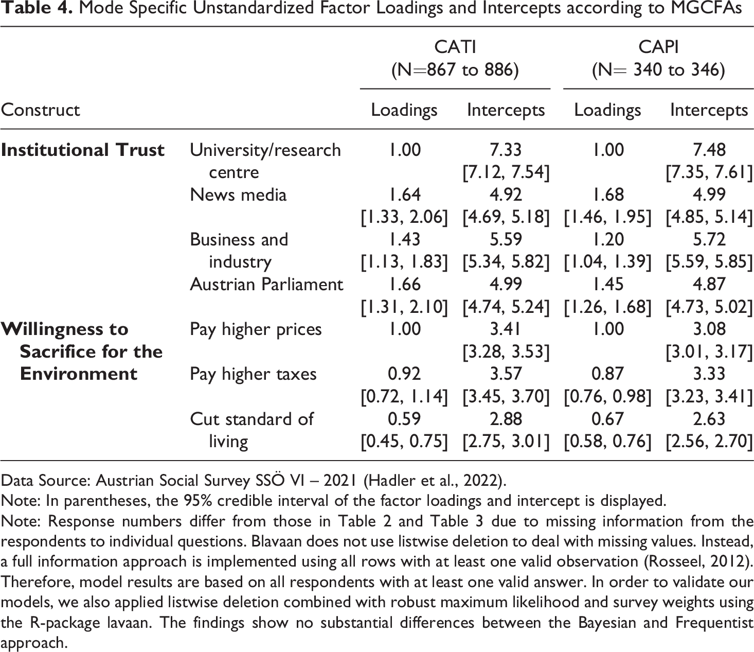
After testing selection effects, we continue to analyse survey-mode differences in the measurement of both social constructs by means of MGCFAs. Table 4 displays the mode-specific unstandardised factor loadings of the four questions on institutional trust and three questions regarding the willingness to pay for the environment as well as the intercepts for the indicators on both social constructs. All factor loadings are substantial and unambiguously positive. Comparing the results across both modes, we see similar point estimates as well as similar uncertainties indicated by the 95% credible intervals.
Mode Specific Unstandardized Factor Loadings and Intercepts according to MGCFAs
Data Source: Austrian Social Survey SSÖ VI – 2021 (Hadler et al., 2022).
Note: In parentheses, the 95% credible interval of the factor loadings and intercept is displayed.
Note: Response numbers differ from those in Table 2 and Table 3 due to missing information from the respondents to individual questions. Blavaan does not use listwise deletion to deal with missing values. Instead, a full information approach is implemented using all rows with at least one valid observation (Rosseel, 2012). Therefore, model results are based on all respondents with at least one valid answer. In order to validate our models, we also applied listwise deletion combined with robust maximum likelihood and survey weights using the R-package lavaan. The findings show no substantial differences between the Bayesian and Frequentist approach.
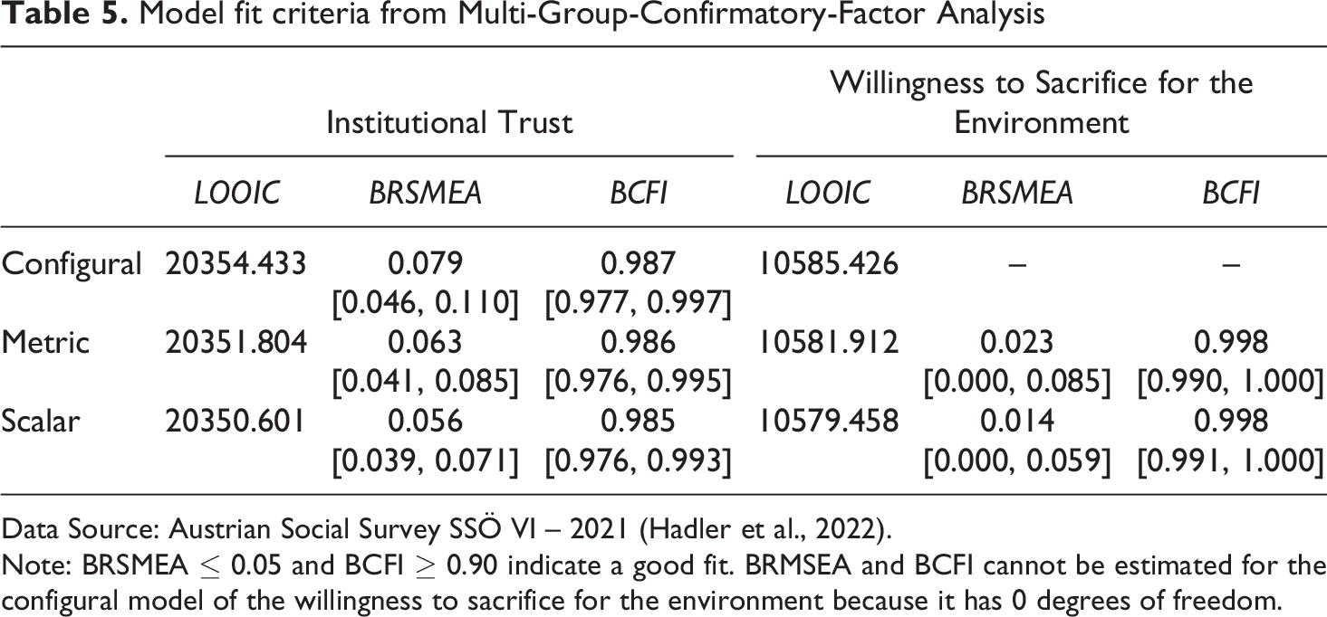
Given the similarities in factor loadings as well as the good fit for the configural invariance model (see first row of Table 5), we continue with testing for metric invariance by placing hard constraints on the factor loadings. Both BRMSEA and BCFI indicate a good fit for the two social constructs (see second row of Table 5). The slightly worse fit of institutional trust can be attributed to the fact that the four institutions are very different, while the responses regarding the willingness to sacrifice for the environment are comparably more consistent. This is also evident given the variance of the averages across the four indicators shown in Table 3. 6 We move on to testing for scalar invariance as shown in the last row of Table 5. For both constructs, additional constraints result in a decrease of BRMSEA indicating a better model fit, while both BCFI distributions remain stable on a high level. Complementarily, LOOIC does not deviate from these results as it gradually decreases with the addition of each constraint. To sum up, the results indicate scalar invariance across both survey modes and thus suggest the absence of mode-effects regarding the measurement structure of both social constructs.
Model fit criteria from Multi-Group-Confirmatory-Factor Analysis
Data Source: Austrian Social Survey SSÖ VI – 2021 (Hadler et al., 2022).
Note: BRSMEA ≤ 0.05 and BCFI ≥ 0.90 indicate a good fit. BRMSEA and BCFI cannot be estimated for the configural model of the willingness to sacrifice for the environment because it has 0 degrees of freedom.
Since blavaan at present does not support survey-weights, we performed robustness checks using the R-package lavaan (Rosseel, 2012) and estimated all MGCFAs using robust Maximum Likelihood and post-stratification weights. Overall results and conclusions are robust and do not deviate substantially from our main findings (see Table A.1 in the appendix).
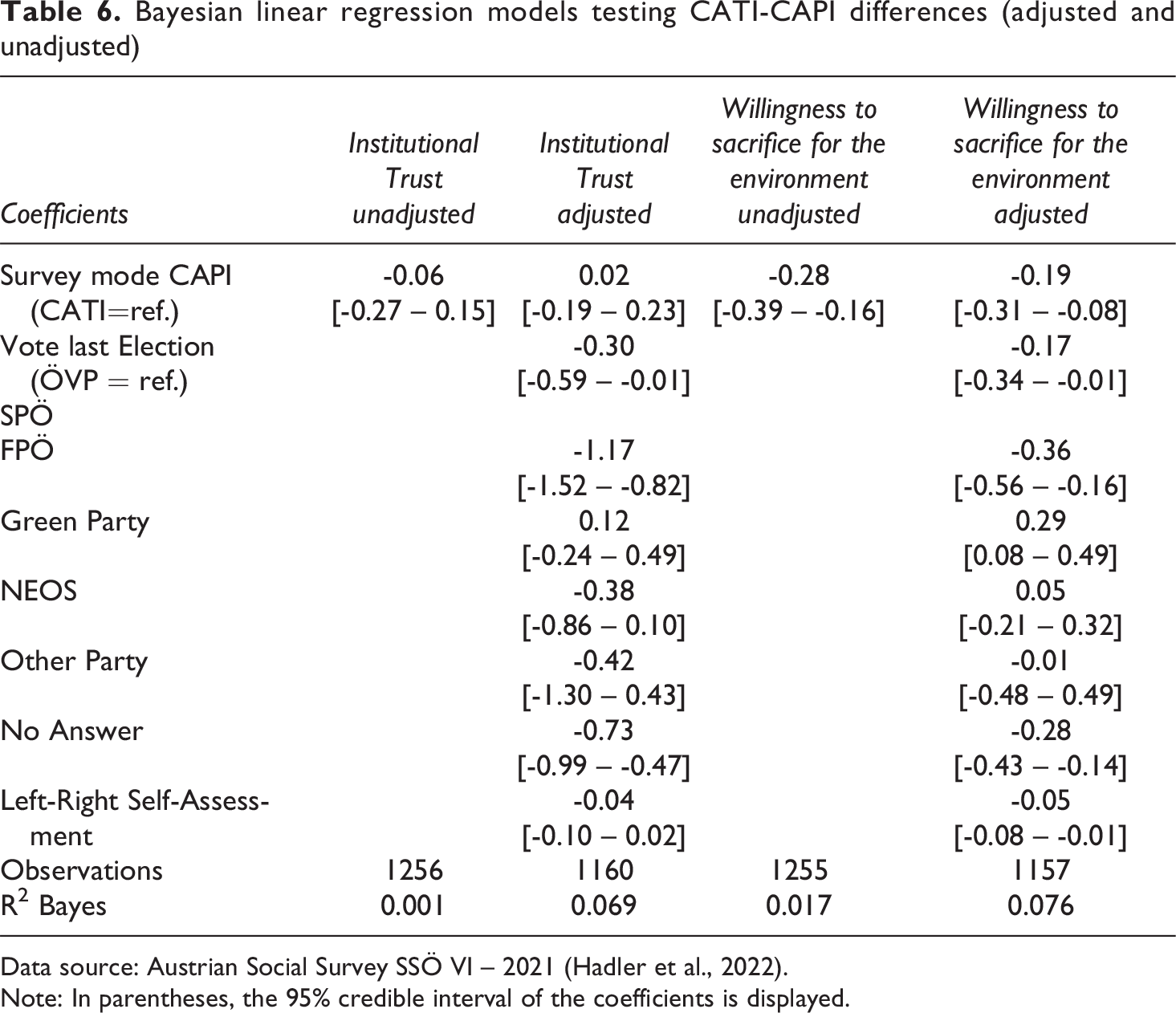
In the next step, we analyse the impact of the mode within a Bayesian linear regression model adjusting for political party preference and political self-assessment on the left-right scale because the analysis of sample composition indicated most distinct mode-differences regarding these two political background variables. We average the answers of respondents for both scales and regress them on our survey-mode variable. The first column in Table 6 shows that while the majority of posterior density is negative, the 95% credible interval also overlaps with positive parameter values. Therefore, mode-differences for institutional trust can be considered negligibly small. The fourth column of Table 6 shows the results for the questions on the willingness to sacrifice for the environment. Here, the 95% credible interval [-0.39 – -0.16] and the posterior distribution solely includes negative parameter values which implies lower willingness to make economic sacrifices for the environment in the CAPI sample than in the CATI sample. However, Bayesian R2 clearly shows that the survey mode does not provide substantial explanatory power for both social constructs.
Bayesian linear regression models testing CATI-CAPI differences (adjusted and unadjusted)
Data source: Austrian Social Survey SSÖ VI – 2021 (Hadler et al., 2022).
Note: In parentheses, the 95% credible interval of the coefficients is displayed.
We continue by adjusting for sociodemographic characteristics to analyse if mode differences in the willingness to sacrifice for the environment are due to an (unwanted) mode effect or caused by differences in the sample composition. We adjust the mode differences for party preferences as well as political left-right self-assessment resulting in a shift in the posterior distribution of the difference towards zero as visualized in Figure 2. The findings show decreasing but still statistically significant differences between modes indicated by the negative limits of the 95% credible interval [-0.31 – -0.08].
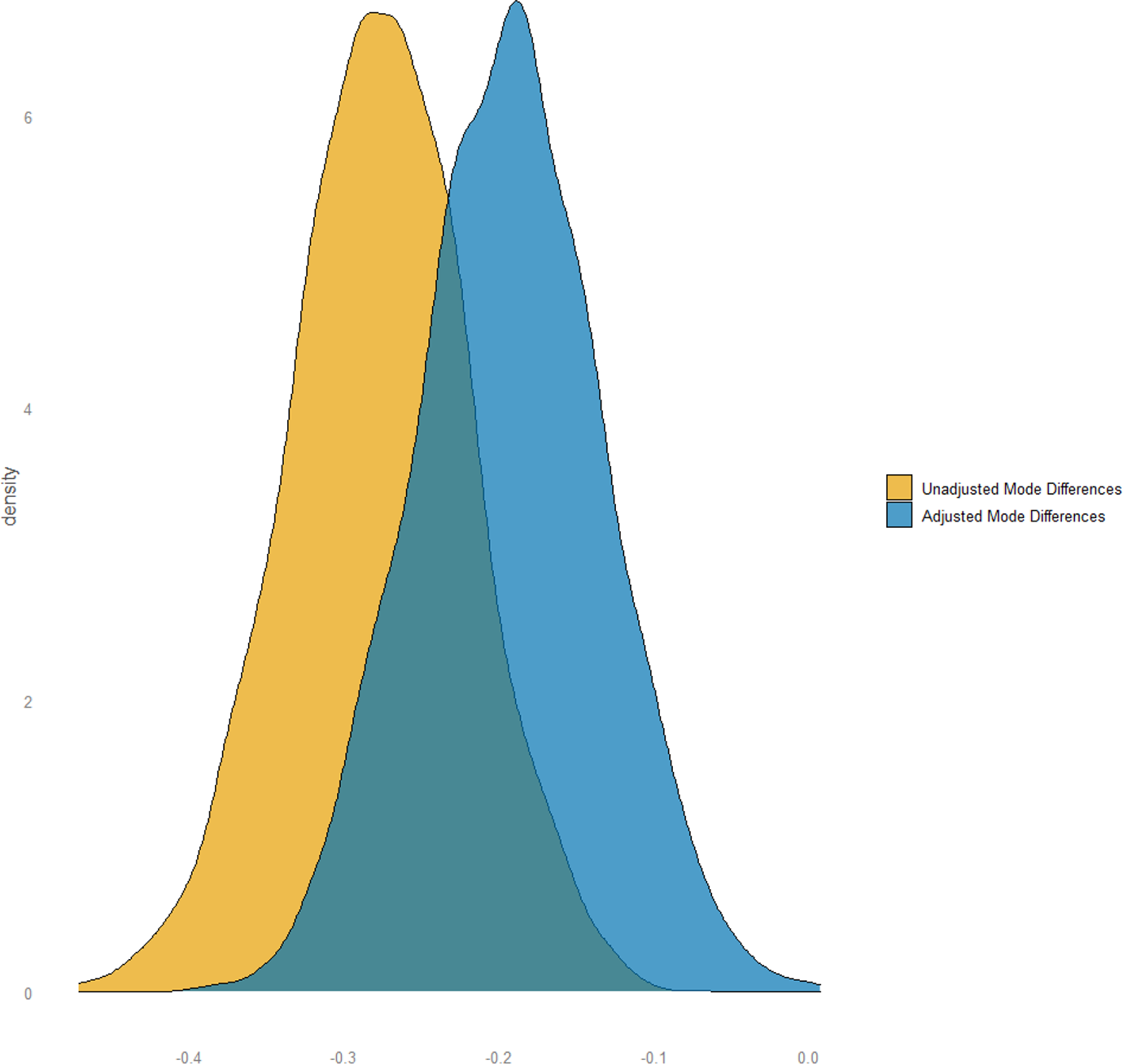
Comparison of adjusted and unadjusted mode differences towards the willingness to sacrifice for the environment
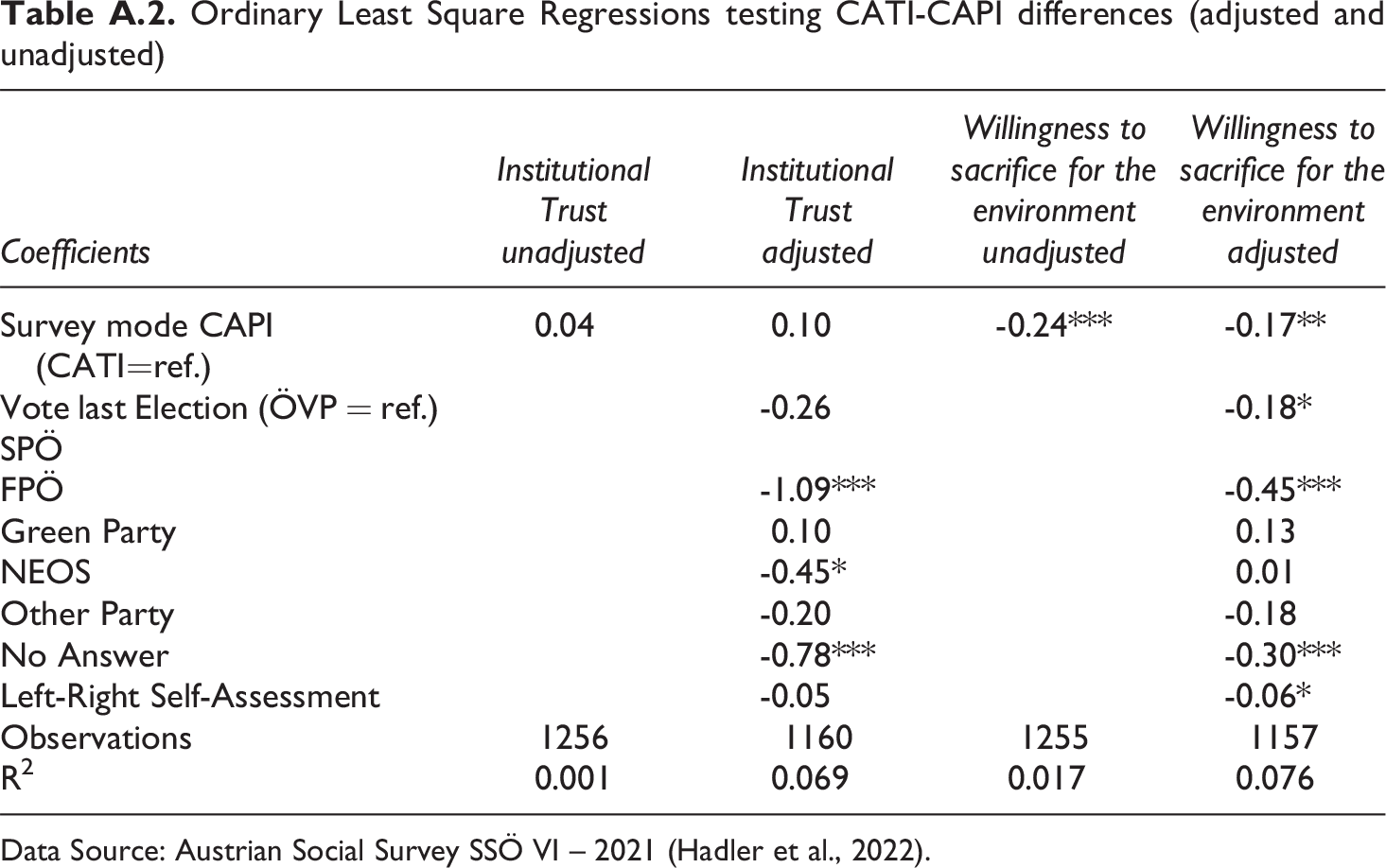
Because the rstanarm package currently does not support survey-weights, we performed robustness checks and estimated all regression models using Ordinary Least Squares combined with post-stratification weights. Again, our results and conclusions are robust and do not deviate substantially from our main findings (see Table A.2 in the appendix).
Discussion
As de Leeuw, Hox, Vannieuwenhuyze, and colleagues have shown in various studies (e.g., de Leeuw et al., 2018; de Leeuw et al., 2008; de Leeuw, 2005; Hox et al., 2015; Hox et al., 2017; Vannieuwenhuyze et al., 2010; Vannieuwenhuyze, 2013), mixed mode surveys have potential to decrease various sources of bias along the total-error framework; however, the combination of different modes also entails risks. Against the backdrop of these prominent studies, our case study aimed at disentangling (desired) selection effects and (unwanted) measurement effects by investigating the two widely used social constructs of institutional trust and willingness to sacrifice for the environment which were conducted in a CATI-CAPI mixed-mode design in the Austrian ISSP Environment (Hadler et al., 2022).
In answering our first research question, if different sociodemographic groups of respondents are attracted by the different survey modes of CATI and CAPI, we can conclude that the analysis of sample composition has shown no substantial mode differences with regard to respondent’s age, educational degree, income, political interest, and gender. It is however, a bit surprising that right-wing voters are more strongly represented in the CAPI sample than in the CATI sample. If it were socially unacceptable to vote the right-wing populists FPÖ, it would be more likely that they seek the greater anonymity of CATI. However, at the time of the survey it was socially acceptable to favour the right-wing populist FPÖ which had regained popularity in larger population groups in Austria. In 2021 somewhat less than 20% indicate that they would have voted them 7 . Another potential cause could be that right-wing voters are less likely to publish their telephone number in a public phone directory and are therefore underrepresented in our CATI sample. However, this point remains speculative as there is no empirical evidence for Austria on this issue. Yet, ultimately, we are unable to explain the higher attraction of right wing-voters in the CAPI mode.
To answer our first research question, we see that in terms of sample composition both modes are very similar. Since we showed that central sociodemographics do not differ between modes, a CATI-CAPI design is not the most effective strategy to attract different target groups. Therefore, we do not generate desired selection effects with this combination of modes in Austria. Especially younger people often favour online surveys which in the very near future will play a crucial role when conducting general population surveys.
With regard to our second research question, to what extent different modes affect response patterns in the sense of measurement effects, the results of Bayesian Multigroup Confirmatory Factor Analysis have suggested strong empirical support for scalar invariance indicating no mode effects on the measurement structure of the social constructs respectively factors. However, further Bayesian linear regression models revealed that even after adjusting for sociodemographics and political party preference and political left-right self-assessment CATI-respondents remained more willingly to sacrifice for the environment than CAPI-respondents. However, it remains questionable whether this difference is a true and substantial mode effect at all. Therefore, we take the analyses at hand as an opportunity to further elaborate on four potential causes that each by itself or simultaneously can cause the observed mode difference. The first explanation is design based and refers to the mixed mode of our case study.
As outlined above, most of the CAPI sample was fielded after the CATI sample which is why public opinion might have changed in the course of the field survey phase. For example, Klösch et al. (2021) showed that the willingness to make economic sacrifices for the environment can be volatile in times of crisis in Austria. Thus, in a mixed mode design, it may become increasingly difficult to disentangle mode effects from actual changes in public opinion as the field period progresses. This could be solved by offering the modes simultaneously which however, might increase the costs of surveys. Instead, other survey-external contextual variables such as the intensity of media coverage on a topic at a specific survey date relevant to the opinion of respondents could be included as additional covariates.
Second, with two political background variables, we included only a small subset of potential covariates in the model. Following Vannieuwenhuyze et al. (2010) also survey related variables such as the preferred survey mode and survey satisfaction show potential for further covariates. Therefore, future research might use a comprehensive set of covariates, beyond sociodemographic variables, when trying to disentangle selection from mode effects.
The third, and for most researchers probably unsatisfactory explanation is that the potential mode effect of the case study at hand resulted by chance. This does not seem too unrealistic given the randomness of sampling procedures. In fact, we cannot be sure whether a repeated survey would have produced the same results. Sampling error cannot be eliminated using finite samples, so it is crucial to quantify and report on the uncertainty in order to get an idea of the potential magnitude of mode effects.
The fourth explanation is that our observed mode differences are indeed a mode effect. However, in accordance with Hox et al. (2015) as well as Martin and Lynn (2011) we also want to emphasize that from the observation of statistically significant mode differences in either measurement structure or response distributions one cannot deduce whether this is a source of bias that significantly distorts potential research outcomes. This requires comprehensive statistical information including a point estimate and at least a measure of dispersion. Moreover, one needs domain-specific knowledge to assess whether a mode effect can significantly bias not only the estimates but also, and more importantly, the conclusions drawn. Given the last two points, we prefer a Bayesian approach to communicate mode-effects as posterior distributions which include more information on the distributional characteristics of mode-effects compared to classic confidence intervals that only describe a range of possible values (Kruschke, 2015). This allows survey methodologists and applied researchers to describe and evaluate mode effects more precisely. Another alternative can be resampling methods such as bootstrapping. This involves drawing repeated samples from the sample size, approximating the sampling distribution of the relevant statistics (Efron, 1979). For mode effects, this allows the distribution of potential mode effects to be estimated and communicated transparently to the reader.
For the case study at hand, it is also important to mention that a mode effect might be associated with the missing use of showcards in the CATI mode. As mentioned above, we only used showcards for the three items measuring the willingness to sacrifice for the environment within the CAPI mode. A possible underlying mechanism of this effect could therefore be the lack of a visual stimulus in the CATI mode meaning that not all response categories are shown at a glance (willingness responses were read out first). This highlights the importance of further exploring the use of showcards and other stimuli in CAPI-CATI mixed mode designs as well as in other survey modes; for future research especially the different ways of (audio-) visual representations in online modes.
To conclude our case study, we would like to emphasize that, according to our results, the CATI-CAPI mix is a reliable mixed-mode design for conducting general population surveys in Austria with non-substantial (unwanted) measurement effects and reasonable sample compositions. However, at the same time we do not observe (desired) selection effects with this mix of modes such as better access to lower educated or older respondents via telephone. Concerning the interpretation and evaluation of mode effects we would like to encourage future research to consider the implications of the four potential causes of observed mode differences discussed in this paper. Given the complexity and the fact that mode effects can be interpreted and evaluated neither monocausally nor without content-related interpretation, it is hardly surprising that the research community yet has not been able to present general thresholds for the evaluation of mode effects.
Footnotes
Declaration of Conflicting Interests
The author declared no potential conflicts of interest with respect to the research, authorship, and/or publication of this article.
Funding
The surveys of the ISSP module on “Environment” and “Social inequality” were financed by the Austrian Federal Ministry of Education, Science and Research.
Notes
Appendix
Ordinary Least Square Regressions testing CATI-CAPI differences (adjusted and unadjusted)
| Coefficients |
Institutional Trust
|
Institutional Trust
|
Willingness to sacrifice for the environment
|
Willingness to sacrifice for the environment
|
|---|---|---|---|---|
| Survey mode CAPI (CATI=ref.) | 0.04 | 0.10 | -0.24*** | -0.17** |
| Vote last Election (ÖVP = ref.) SPÖ |
-0.26 | -0.18* | ||
| FPÖ | -1.09*** | -0.45*** | ||
| Green Party | 0.10 | 0.13 | ||
| NEOS | -0.45* | 0.01 | ||
| Other Party | -0.20 | -0.18 | ||
| No Answer | -0.78*** | -0.30*** | ||
| Left-Right Self-Assessment | -0.05 | -0.06* | ||
| Observations | 1256 | 1160 | 1255 | 1157 |
| R2 | 0.001 | 0.069 | 0.017 | 0.076 |
Data Source: Austrian Social Survey SSÖ VI – 2021 (Hadler et al., 2022).