
Abstract
We examine the effects on survey estimates of extended interviewer efforts to gain survey response, including refusal conversion attempts and attempts to make contact with difficult-to-contact sample members. Previous research on this topic has identified that extended efforts do appear to affect estimates, and in ways that seem consistent with bias reduction. We extend the previous research in three ways. First, we provide the first study of changes over time in the effects of extended efforts on estimates. We study change in the UK over a ten-year period. Second, we use a more precise measure of the difficulty of contact and third, we assess the effects of extended efforts conditional on weight adjustments for non-response estimates as well as on unweighted sample statistics.
Introduction
Non-response is a serious concern for survey researchers. The aspect of central concern is the possibility that non-response may be systematic with respect to key survey estimates, leading to bias in those estimates (Lynn, 2008). However, while survey methodologists have learnt a lot about ways in which features of survey design and implementation can affect response rates, effects on non-response bias are generally much harder to predict or to identify (Groves, 2006). Consequently, surveys typically go to great efforts to maximise response rates in the hope that this will reduce non-response bias, rather than specifically targeting bias.
A technique designed to maximise response rates to face-to-face surveys involves making extended field efforts (Lynn et al., 2002). These extended efforts include additional attempts to persuade sample members who initially refuse to take part and additional visits to try to contact sample members who have not been contacted after “normal” or “minimum” field procedures have been completed. A couple of decades ago, survey organisations used to implement such extended efforts only in extremis; that is when a survey was unexpectedly suffering from an unusually low response rate. But these extended efforts are now seen as good practice for all scientific studies for which accuracy of estimation is important. These extended efforts can account for a sizeable proportion of the field budget and must therefore be justified in terms of cost-effectiveness. There is some evidence that the respondents for whom most effort is required are distinct in relevant characteristics. For example, in surveys of sexual behaviour in both the UK and France (Copas et al., 1997; Firdion, 1993) it has been found that obtaining the participation of the most difficult respondents reduces non-response bias in key estimates of sexual behaviour. Central aims of this paper are therefore to establish the extent to which extended efforts, a) improve response rates, and b) reduce non-response bias. An additional aim is to assess the extent to which these factors may have changed since a decade previously. Regular reassessment of the justification for survey design features is warranted in a changing world where propensities to be contacted and propensities to co-operate with surveys are likely to change both over time and between sample subgroups. As in many countries, the past decade in the UK has seen response rates decline on several major surveys (Betts and Lound, 2010: 7). Although there is some evidence that it has become more difficult to contact people at home, the decline in response is mainly due to an increase in refusals. To tackle both forms of non-response, survey organisations have had to invest greater field resources and to consider new tactics. For example, analysis of process data from general population face-to-face surveys carried out by NatCen Social Research shows that the mean number of interviewer visits before a final outcome of non-contact is recorded (not including reissues to a different interviewer) was 6.6 in 1995-1996, 7.6 in 2006 and 8.0 in 2009-2010 (own analysis).
A decade ago, Lynn and Clarke carried out a study with similar aims to ours. They concluded that extended field efforts appeared to be justified in terms of bias reduction. In particular, they identified significant bias reduction in all three of the surveys they examined due to contacting those who were initially difficult to contact. The impact of extra efforts to convert initial refusals was less clear-cut: refusal conversion appeared to affect the estimates of financial variables but there was no systematic impact on estimates related to health or attitude variables. We replicate the methodology of Lynn and Clarke using data from the same three large national general population surveys, namely the Health Survey for England (HSE), the British Social Attitudes Survey (BSAS) and the Family Resources Survey (FRS). We use data from 2006 and 2007 for the HSE and BSAS, and 2007 for the FRS. Using the same methodology and the same surveys, each of which are still carried out by the same organisation as ten years previously, gives us a strong basis for drawing conclusions about changes in effects over this period. The diverse nature of the three surveys allows us to assess effects on bias for three distinct types of survey estimates – health measures, attitudinal measures and financial measures – as well as demographic indicators.
Additionally, we extend the work of Lynn and Clarke in two important ways. First, we use a more precise measure of the difficulty of contact, which was not available at the time of the earlier study, and we assess the sensitivity of the findings to the choice of measure. Second, we also assess the effect of extended efforts on weighted estimates, to establish the extent to which weight adjustments for non-response can overcome any differential non-response bias. If weighting were able to achieve the same bias-reduction effects as extended field efforts, this may greatly reduce the justification for investing in expensive field efforts.
Methods
The Data
All three surveys used by Lynn and Clarke (2002) are currently still ongoing, and we are therefore able to utilise more recent years of these same surveys for our analysis. We have used the 2006 and 2007 rounds of the BSAS and the HSE, and the 2007 round of the FRS. Lynn and Clarke chose these surveys because they differ in terms of subject matter, respondent burden, respondent selection criteria, response rates, and the extent to which they rely on extended interviewer efforts. The fieldwork for the first two surveys is conducted wholly by NatCen, while the FRS has fieldwork conducted jointly by the Office for National Statistics (ONS) and NatCen. Consequently, we have only used one half of the FRS data for our analysis due to data availability. This follows the approach of Lynn and Clarke. The sample is split randomly between the two organisations in such a way as to keep its stratified random sampling properties.
The BSAS consists of a face-to-face computer-assisted interview followed by the administration of a paper self-completion questionnaire, with fieldwork carried out from June to October of each survey year. It measures attitudes, values and beliefs on a range of political and social issues and is a stratified random probability sample of private households within Britain selected from the Postcode Address File (PAF). One adult aged 18 or over is selected per household to answer the questionnaire (both the face-to-face component and the self-completion component). In 2006 and 2007, the BSAS interviewed approximately 4,000 individuals in each year, with response rates of 54 percent and 51 percent respectively.
The HSE comprises a series of annual surveys covering the adult population aged 16 and over living in private households in England. The survey provides regular information that cannot be obtained from other sources on a range of aspects concerning the public’s health and many of the factors that affect health. As with the BSAS, it is a multi-stage stratified probability sample selected from the PAF. However, unlike the BSAS, all adults aged 16 years or older in each sample household are selected for the face-to-face interview. In 2006, there were 14,142 interviews with adults representing a response rate of 61 percent, and in 2007 6,882 adults were interviewed with a response rate of 58 percent.
The FRS has a similar sample design to the BSAS and HSE (multistage stratified random sample from the PAF) and is representative of adults aged 16 and above (non-dependents). As with the HSE, all adults in the household are interviewed, and the annual target sample size is 24,000 households. The face-to-face interviews are mainly concerned with income, living standards and related issues. The data analysed here are from the 2007-08 FRS, which had an achieved response rate of 58 percent (23,121 fully co-operating households). A slight difference between the surveys in geographical coverage should be noted: BSAS and FRS each cover England, Scotland and Wales, whereas HSE is restricted to England. The population of England accounts for around 85 percent of the total population of England, Scotland and Wales.
For all three surveys, interviewer effort is captured through the sample management system. Interviewers were asked to record for each address the date, time and outcome of each visit made. The outcome categories were: no reply, contact made, appointment made, any CAPI interviewing done, or other. The “other” category includes refusals and ineligibles, thus from this code once responding addresses are isolated we can deduce whether or not any visits to these addresses resulted in a refusal. This information was captured on the paper-based Address Record Form and subsequently entered into the electronic sample management system at regular intervals throughout the fieldwork period.
Definitions
Following Lynn and Clarke, “reluctant” responding households are classified as all those households that initially refused to take part in the survey but subsequently agreed to be interviewed after being reissued to another interviewer. The “difficult-to-contact” households are all those households that required 6 or more visits before an interview was obtained. The “reluctant” and “difficult-to-contact” households when combined to form the “hard-to-get” group (see Figure 1) – that is, these cases were the ones where extended efforts were needed on the part of the interviewer. We term all responding households where extended efforts were not required as “easy-to-get”, though it must be borne in mind that this is a relative term. Figure 1 is used to illustrate this categorisation (Lynn and Clarke, 2002).
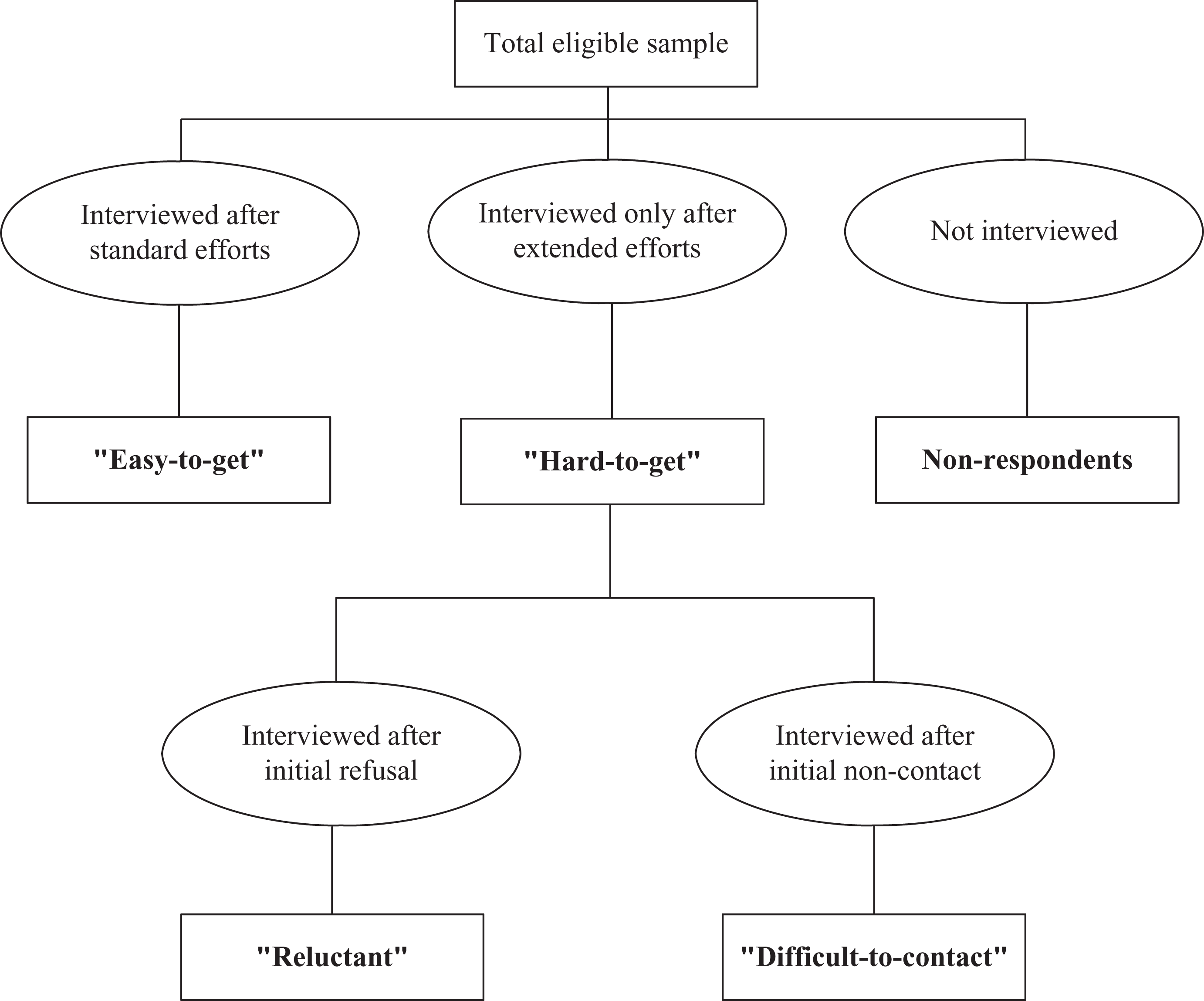
Classification of households.
We use Lynn and Clarke’s measure of “difficult-to-contact” for comparability as we wish to make inferences about change over time. Lynn and Clarke had recognised that total number of visits was not ideal as a measure of “difficult-to-contact”, particularly because successful interviewer strategies involve leaving and returning on another occasion to avoid prompting a refusal. Hence, total number of visits is influenced by reluctance as well as ease of contact. Their preferred definition would have been based on whether or not contact was made before 6 visits. Unfortunately Lynn and Clarke were unable to use this measure for all the surveys they analysed as the information needed was not recorded in an electronic format at that time.
Lynn and Clarke were able to use paper-based records for one survey (BSAS 1998) to determine the difference this alternative definition made to the percentage classed as “difficult-to-contact”. They concluded that: “The extent to which total number of visits may mislead as a measure of difficulty in contacting households is obvious…of the 4.6 percent of households for which 10 or more visits were needed... less than half required 10 or more visits to make contact with the household…” However, Lynn and Clarke did not compare estimates of bias using this alternative definition of "difficult-to-contact" with estimates based on total number of calls.
Since the introduction of routine electronic recording of the outcome of every visit made to an address during the fieldwork process, we can now use the preferred measure of difficulty of contact. We extend the earlier research by replicating all analysis using this preferred definition and compare the results to provide an assessment of the sensitivity of the findings to the measure used. Whereas Lynn and Clarke’s measure was based on the total number of visits to a household, our preferred measure is based on the number of visits until contact is first made (for HSE 2006 and 2007, BSAS 2006 and 2007, and FRS 2007). For example, if contact was made with a household on the fourth visit but the interview was not conducted until the seventh visit, the previous analysis would have classed this household as “difficult-to-contact” based on v=6 (if they had never refused on any of the visits). However, in our preferred measure this household will be classified as “easy-to-get”, since contact was made before the sixth visit (albeit without an interview taking place on that particular visit).
Weighting for Non-response Bias
Lynn and Clarke (2002) studied the effects of extended field efforts on estimates based on unweighted data. But typically researchers make weighting adjustments for non-response and use weighted estimates. It may be expected that effective non-response weighting should compensate for at least some of the bias that would otherwise be reduced by the use of extended field efforts. It is therefore of interest to know if and how weighted estimates following extended efforts differ from weighted estimates in the absence of extended efforts. To make this comparison, the overall responding sample and the “easy-to-get” respondent sample are each independently weighted according to an identical weighting scheme. We would expect this weighting to reduce differences in estimates between the samples, to the extent that the weighting variables are associated with the target variables of interest. For each survey, the weighting scheme is the one used on the actual survey to adjust for differential non-response, and is as described below.
The weighting for the BSAS first involves fitting a logistic regression, with the dependent variable indicating whether or not the selected individual responded to the survey. A number of area-level and interviewer observation variables are used to model response, such as Government Office Region (GOR), dwelling type, condition of the address, and if the selected address has entry barriers. The resultant non-response weights then receive a post-stratification adjustment so that the weighted sample matches the population in terms of age, sex and region (using ONS mid-year population estimates).
The HSE weighting involves calibration weighting to ensure that the weighted distribution of household members in participating households matches ONS mid-year population estimates for age/sex groups and GOR. The aim of the calibration is to reduce non-response bias resulting from differential non-response at the household level. Adults in responding households are then given a non-response weight using logistic regression to reduce bias arising from individual non-response. Age group by sex, household type, GOR, and social class of the household reference person are entered into the model as covariates.
The FRS weighting does not involve logistic regression weighting but does involve calibration at different levels: individual, benefit unit, and household. The calibration variables used for individuals were age, sex and GOR. For benefit units, they were presence of children (England and Wales with dependent children, Scotland with dependent children), and lone parents by sex of the parent. For households, the variables used were tenure, council tax band and region (London, Scotland and all other England and Wales).
Analysis methods
Estimates of marginal biases that would have been present in the survey, had extended efforts not been made, were calculated as the percentage or mean for the “easy-to-get” group less the percentage or mean for the overall responding sample. To test the significance of marginal bias estimates, we perform t-tests between the “easy-to-get” group and the “hard-to-get group” (see Appendix), not taking into account the complex sample design of each survey (as this is what Lynn and Clarke did). For the extension analysis, on refining the measure of “difficult-to-contact” and assessing the impact on weighted estimates, we performed t-tests between the “easy-to-get” group and all respondents, taking into account the complex sampling (clustering and stratification) of each survey. Additionally, weighting was applied when running the t-tests. SPSS version 18 and Stata version 10 were used for the analysis. Missing values were dealt with using pair-wise deletion. Significance was evaluated at the 95 percent level, although significance at the 90 percent level is also indicated.
Results
Change over Time
We replicate the approach of Lynn and Clarke (2002) in presenting findings based on the definition of “difficult-to-contact” if the household was only interviewed after 6 or more visits (v=6), plus sensitivity analyses using v=8 and v=10. Most of the broad patterns found using v=6 remained for v=8 and v=10. In some cases, the differences between the “difficult-to-contact” and “easy-to-get” households become smaller as the definition of “difficult-to-contact” is made more restrictive, but all of the differences that were significant with v=6 remained significant with v=8 and v=10 for the demographic variables in both surveys. For the remainder of this paper, we only present results based on v=6.
Table 1 presents estimates of the proportion of sample households classified as “difficult-to-contact”, “reluctant”, “hard-to-get” and “easy-to-get”, for HSE, BSAS and FRS respectively. Estimates are averaged across the 2006 and 2007 surveys and are compared with estimates averaged across the years examined in Lynn and Clarke (2002), which are 1996 and 1997 in the case of HSE; 1995, 1996 and 1998 in the case of BSAS; and 1997 for the FRS.
Distributions of “difficult-to-contact”, “reluctant” and “easy-to-get” households across surveys and years.
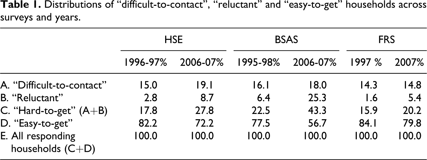
The proportion of the eligible sample classified as “difficult-to-contact” has, on average, increased for all three surveys over the intervening decade. It increased from 15.0 percent to 19.1 percent for HSE and from 16.1 percent to 18.0 percent for BSAS. The increase was smaller for the FRS, from 14.3 percent to 14.8 percent.
The proportion of “reluctant” households increased even more dramatically over this period, more than tripling on all three surveys: from 2.8 percent to 8.7 percent for the HSE, from 6.4 percent to 25.3 percent for BSAS and from 1.6 percent to 5.4 percent for FRS.
Although the proportion of converted refusals has increased over the years for all surveys, it is important to note that the proportion of reissued cases has also increased. In other words, a similar proportion of households 10 years ago may have been “reluctant” but no efforts were made to convert them after their initial refusal. Therefore, we cannot be sure to what extent the observed change reflects increasing reluctance to take part in surveys rather than increasing efforts made to persuade reluctant sample members to take part.
Lynn and Clarke (2002) identified a higher prevalence of “difficult-to-contact” households for the BSAS surveys than for the HSE and FRS. However, by 2006-07 this difference had reversed. This change, and other differences between the surveys, are likely to be caused largely by differences in fieldwork practices across surveys and across years, though the difference in geographical coverage of the surveys – noted earlier – may also have a modest impact.
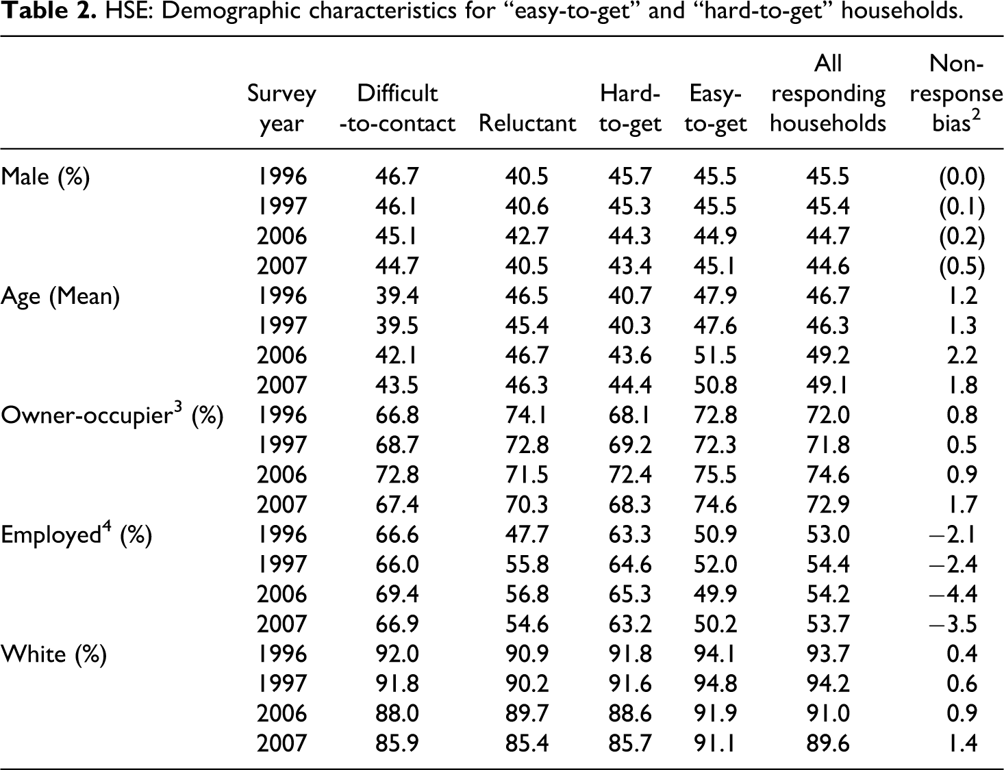
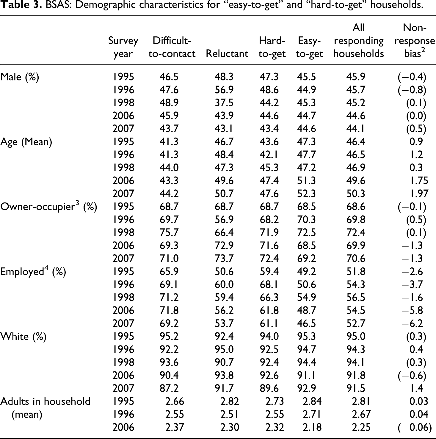
Tables 2, 3 and 4 show, for the three surveys respectively, the five socio-demographic variables presented in Lynn and Clarke (2002), with an estimate of the marginal bias that would have occurred had extended efforts not been made. For all three surveys, the conclusions drawn in the Lynn and Clarke paper broadly remain for the later survey years. Respondents in “hard-to-get” households are considerably younger, on average, than those in “easy-to-get” households (this difference has increased in both the HSE and BSAS 1 ). Respondents in “hard-to-get” households are also much more likely to be employed than those in “easy-to-get” households, and the marginal bias for employment has increased noticeably since the earlier years of all three surveys. The “difficult-to-contact” remain the group with the highest percentage who are employed. For the HSE and FRS, “hard-to-get” households are also less likely to be owner-occupiers or white, findings similar to those of Lynn and Clarke (2002) (there was no significant difference in the proportion of owner occupiers for the FRS in 1997). For the BSAS, “hard-to-get” households are more likely to be owner-occupiers in both 2006 and 2007, and less likely to be white in 2007 only. The latter conclusion is consistent with Lynn and Clarke (2002), but a statistically significant difference between “hard-to-get” and “easy-to-get” households in terms of the owner-occupier variable is a new finding. Prior to 2006, the BSAS survey reported a higher prevalence of owner-occupiers in the “easy-to-get” households (although not significant), whereas this trend has reversed in 2006 and 2007.
HSE: Demographic characteristics for “easy-to-get” and “hard-to-get” households.
BSAS: Demographic characteristics for “easy-to-get” and “hard-to-get” households.
FRS: Demographic characteristics for “easy-to-get” and “hard-to-get” households.

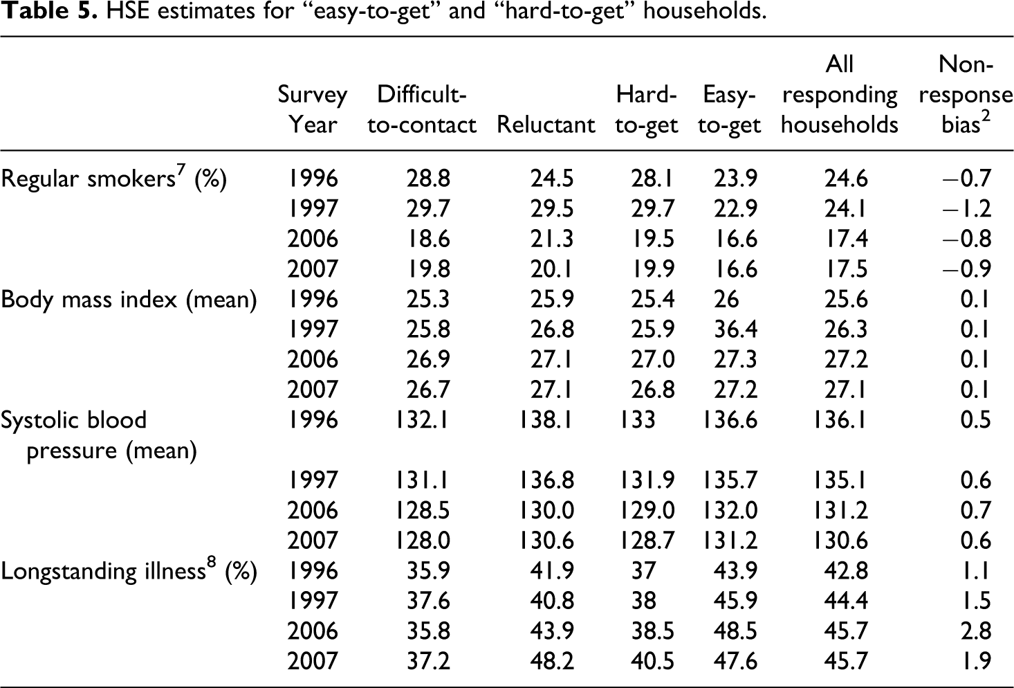
Though we have seen that extended efforts significantly change the distribution of demographic characteristics, the question remains whether or not this translates into bias reduction for key survey estimates. For each of the three surveys, we present estimates of a number of key survey indicators in Tables 5, 6 and 7 respectively, each estimated separately for the “difficult-to-contact”, “reluctant”, “hard-to-get” and “easy-to-get” households. Again, differences between “hard-to-get” and “easy-to-get” households are very similar to those found by Lynn and Clarke (2002) ten years earlier. The HSE data show that persons in “hard-to-get” households are more likely to be regular smokers, are less likely to have a long-standing illness, and are likely to have lower body mass index and lower blood pressure. 5
HSE estimates for “easy-to-get” and “hard-to-get” households.
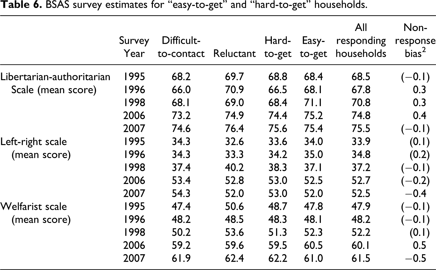
BSAS survey estimates for “easy-to-get” and “hard-to-get” households.
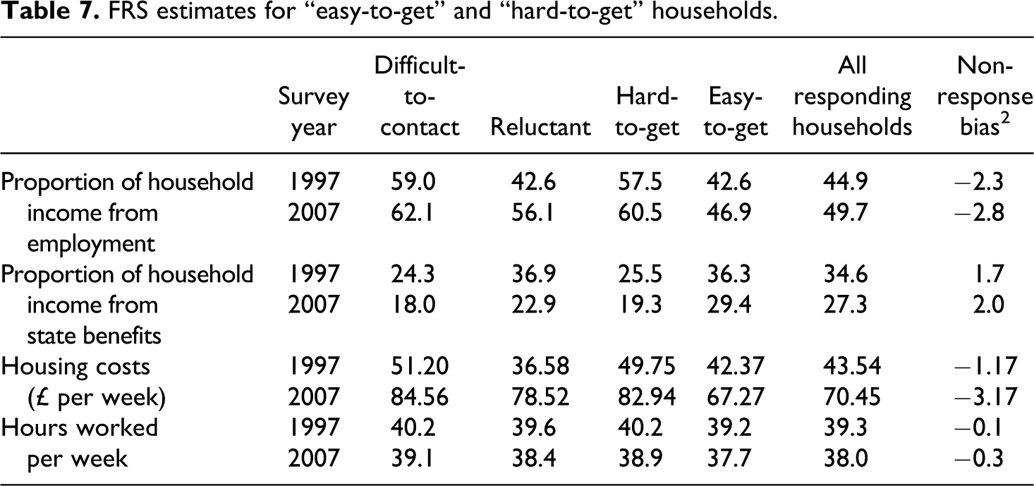
FRS estimates for “easy-to-get” and “hard-to-get” households.
For the BSAS, we see only small differences in attitude scores between persons in “easy-to-get” households and those in “hard-to-get” households. Although there is now a significant difference for some measures (most were not significant in Lynn and Clarke), the differences are small in substantive terms.
For the FRS, persons in “hard-to-get” households work more hours per week, on average, than those in “easy-to-get” households. They also belong to households that obtain a larger proportion of their household income from employment and a smaller proportion from state benefits. “Hard-to-get” households also have higher housing costs than “easy-to-get” households, on average. 6
Overall, our findings are consistent with Lynn and Clarke (2002). The differences in demographic characteristics between respondents in “hard-to-get” households and those in “easy-to-get” households have changed little over the decade. “Hard-to-get” respondents remain more likely to be younger, employed, and non-white. The differences in survey variables for the HSE between the “hard-to-get” and “easy-to-get” households also remain.
However, both the “reluctant” and “difficult-to-contact” groups now make up a larger proportion of responding households than they did 10 years ago. While some of this increase may be due to a genuine increase in the proportion of the population who are reluctant to take part in surveys, some could be ascribed to changes in survey design, notably changes in fieldwork priorities and an increased use of extended efforts such as refusal conversion attempts. Lynn and Clarke (2002) state that: “A clear message is that extended field efforts appear justified in terms of bias reduction”. This conclusion is substantiated by the results presented here. Indeed, it appears that greater field efforts were required in 2006-07 to make similar bias reductions, compared to 1996-98.
Refining the Measure of “Difficult-to-contact”
We noted earlier a shortcoming of the measure of difficulty of contact used in Lynn and Clarke (2002). In this section, we compare results using that measure with results based upon our preferred measure. We replicate the analysis of Tables 2, 3 and 4 using our preferred measure. With this measure, we find that differences between “difficult-to-contact” and “easy-to-get” households are very similar to those based on Lynn and Clarke’s measure, with the one exception of gender, for which differences are more pronounced with the new measure (results not shown, for reasons of space). Regarding gender, we find that the “difficult-to-contact” are more likely to be male (all comparisons other than BSAS 2007) and that all of these differences are greater than those observed with the Lynn and Clarke measure. The percentage point differences are +3.4, +6.5, +6.9 and +1.7 for HSE 2006, HSE 2007, BSAS 2006 and FRS 2007 respectively, compared to +0.2, -0.4, +1.2 and +1.0 respectively using Lynn and Clarke’s measure.
With the new measure, the estimates of marginal bias are smaller in magnitude for most variables for all three surveys, but remain significant. There are just three variables for which the marginal bias is no longer significant (age for both years of BSA and ethnic group for FRS), though there is also one for which the bias becomes significant (ethnic group for BSAS 2006).
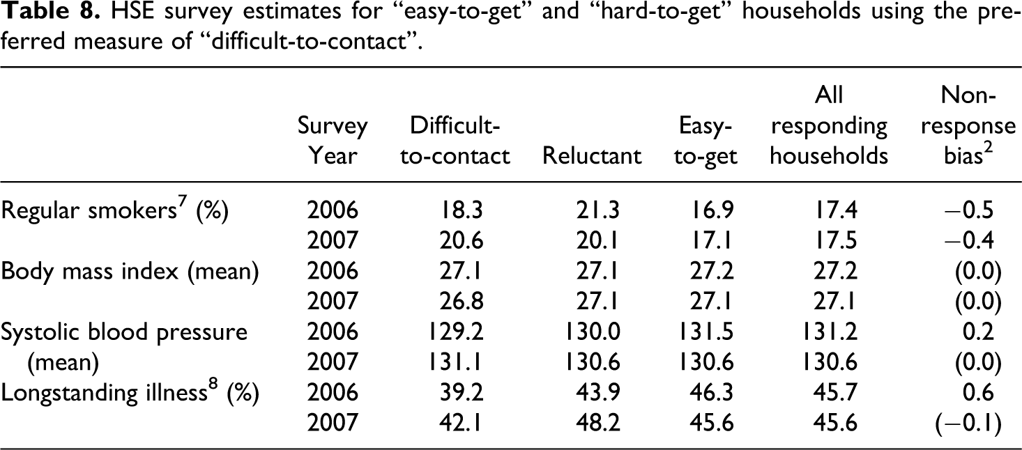
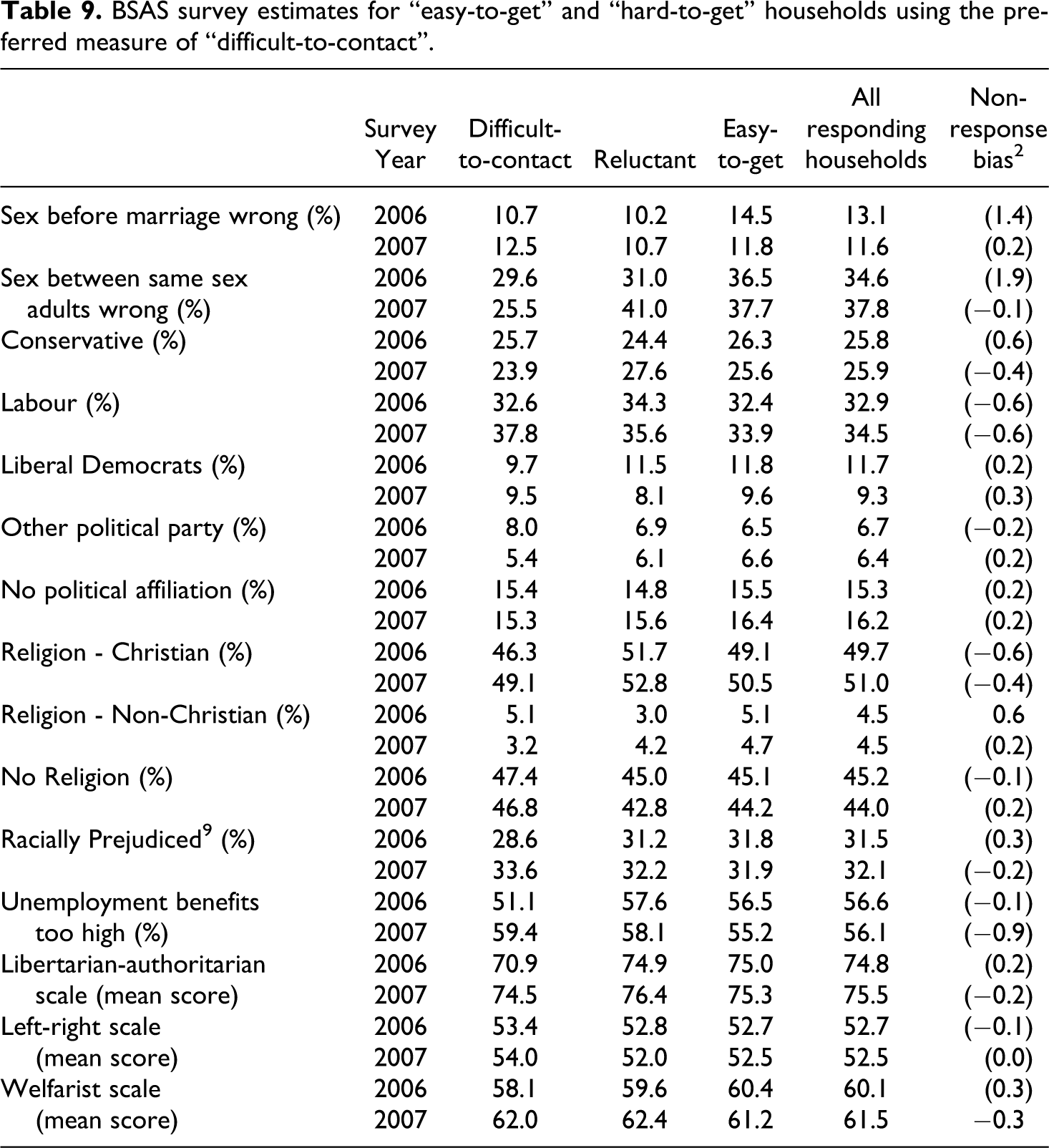
Tables 8, 9 and 10 present the survey-specific estimates using the new definition of “difficult-to-contact” for HSE, BSAS and FRS respectively. For these key measures, the marginal bias estimates are now smaller compared to when we used Lynn and Clarke’s definition of “difficult-to-contact” (Tables 5, 6 and 7). While these smaller differences remain significant for the HSE 2006, all – bar regular smoking – become non-significant in the HSE 2007. The “hard-to-get” remain more likely to be regular smokers than the “easy-to-get”. This was true for both “reluctant” households and “difficult-to-get” households.
HSE survey estimates for “easy-to-get” and “hard-to-get” households using the preferred measure of “difficult-to-contact”.
BSAS survey estimates for “easy-to-get” and “hard-to-get” households using the preferred measure of “difficult-to-contact”.
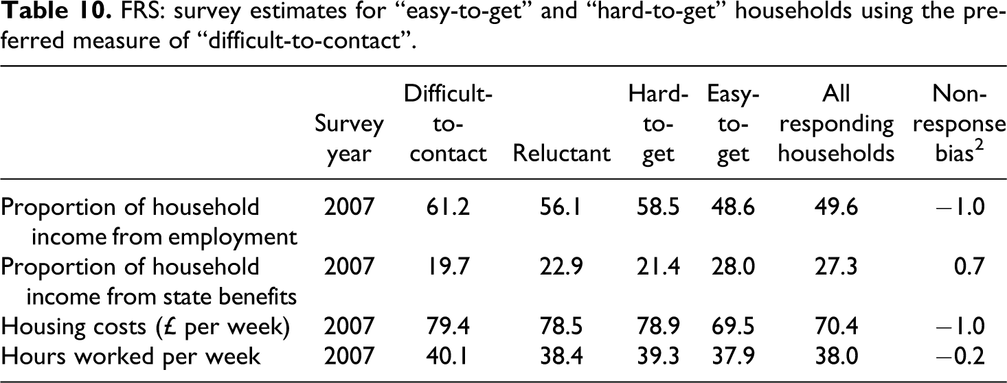
FRS: survey estimates for “easy-to-get” and “hard-to-get” households using the preferred measure of “difficult-to-contact”.
Using the original measure of “difficult-to-contact”, little variation was observed between “easy-to-get” and “hard-to-get” households for the BSAS. With the preferred measure, some additional attitudinal variables consistent from a time series perspective were added. The additional variables were selected on the basis of length of time series, frequency of use by analysts and availability.
Bias estimates are smaller in magnitude with the preferred measure of “difficult-to-contact”, with the exception of the libertarian-authoritarian scale in 2007 (this bias estimate has also become significant at the 10 percent level whereas before it was not significant). The two biases, which were significant at the 10 percent level previously, have now become non-significant, while the bias associated with the welfarist scale in 2006 is now only significant at the 10 percent level. The only remaining bias at the 5 percent level is that associated with the welfarist scale in 2007.
With respect to the additional attitude variables, there seems to be little overall or reluctant non-response bias when considering self reported no religion, party identification, racial prejudice or attitudes to unemployment benefits. In 2006, “easy-to-get” respondents were significantly more likely to agree that sex before marriage was wrong (although this was only significant at the 10 percent level), and were more likely to belong to non-Christian religions.
For the FRS, while the magnitude of the marginal bias is reduced for all four of the survey variables examined, they all still remain significant with the preferred definition of “difficult-to-contact”.
These results give mixed evidence for the need for extended efforts. Only a few variables (being a regular smoker, systolic blood pressure, having a longstanding illness, being of non-Christian denomination and the attitudinal question towards sex before marriage) have significant overall bias remaining in the 2006 surveys. However, the bias in most of the survey specific variables disappears in the HSE and BSAS 2007. Nonetheless, the bias remains in all variables examined in the FRS 2007.
To illustrate the importance of making several visits to attempt to make contact with a household, Figure 2 plots the percentage employed by when first contact was made at an address. If analysis were limited to households where contact was made at the first or second visit, we would obtain an estimate of the percent employed of 49.5 percent. Using all households where contact was made before or on the seventh visit, the estimate is 53.9 percent. Only once eight call attempts have been made does the estimate of the percent employed stabilise at around 54.2 percent. It therefore appears that efforts after the eighth visit (to make first contact) will not reduce the bias much, but calls before and including the eighth may be justified in terms of bias reduction.
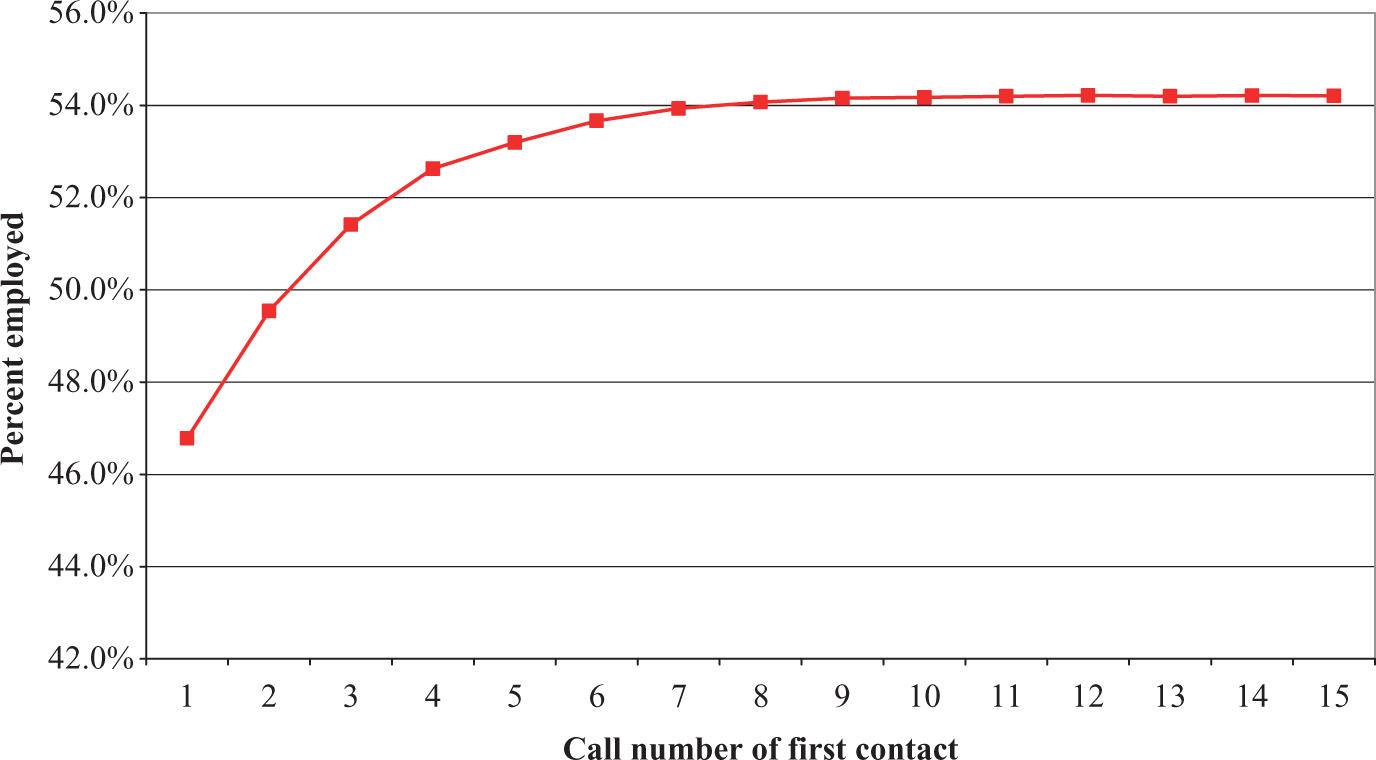
Estimates of percent employed by when first contact was made at an address.
With our preferred measure of “difficult-to-contact” (based on the number of calls to first contact), we largely find that the conclusions drawn by Lynn and Clarke (2002) remain for the demographic variables (albeit with smaller estimates of bias reduction due to extended efforts). That is, extended field efforts both in the form of converting refusals and making numerous (perhaps as high as or higher than 8) calls to achieve contact are needed to reduce the risk of bias. However, the evidence for survey-specific variables becomes more mixed. In 2007, using contact after six calls as the definition of “difficult-to-contact”, limited bias reduction is achieved for most of the survey variables by making additional call attempts. This suggests that calls after the sixth call to make first contact with a household may have little impact on the risk of bias in survey measures.
Impacts on Weighted Estimates
In this section we compare the “easy-to-get” households with all responding households in terms of weighted estimates. The “easy-to-get” households (using the adjusted definition as set out in the previous section) have been weighted as if they were the final respondent pool, using the same weighting procedure as used for all respondents in each survey, and as described earlier.
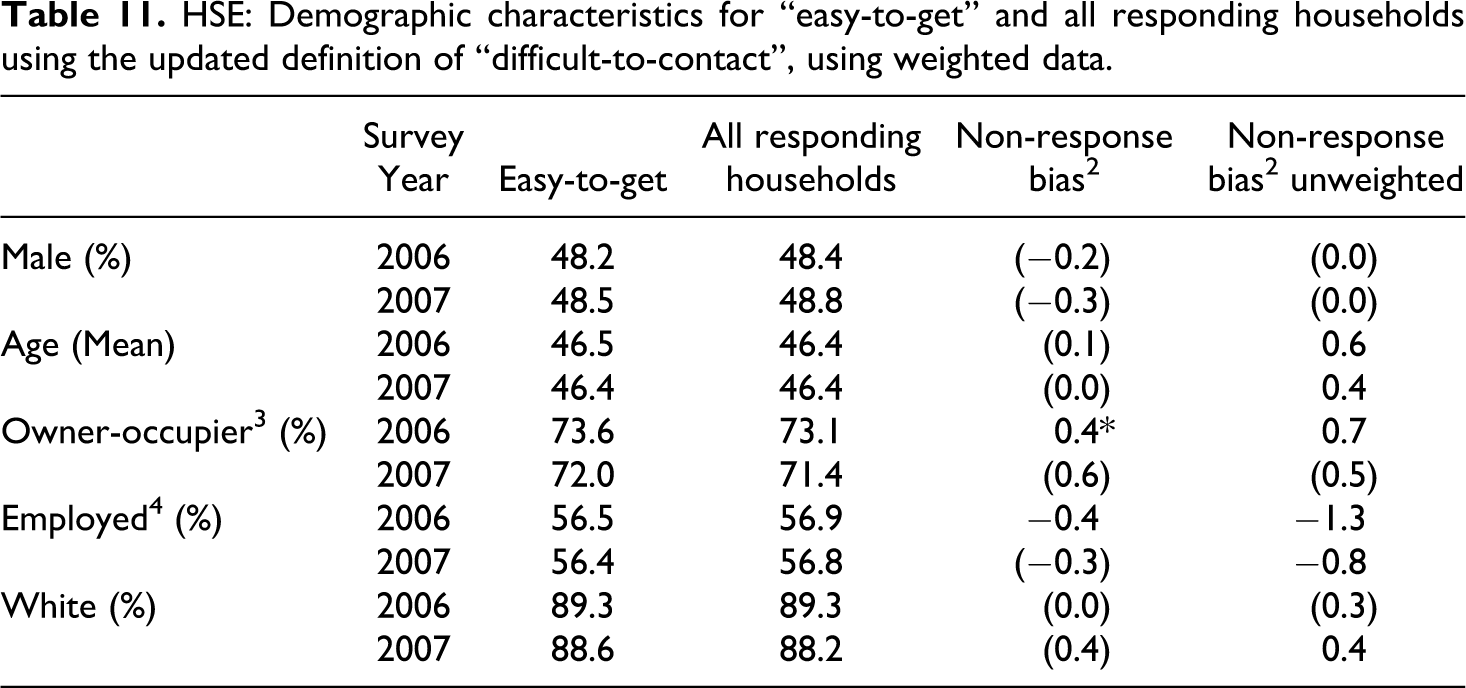
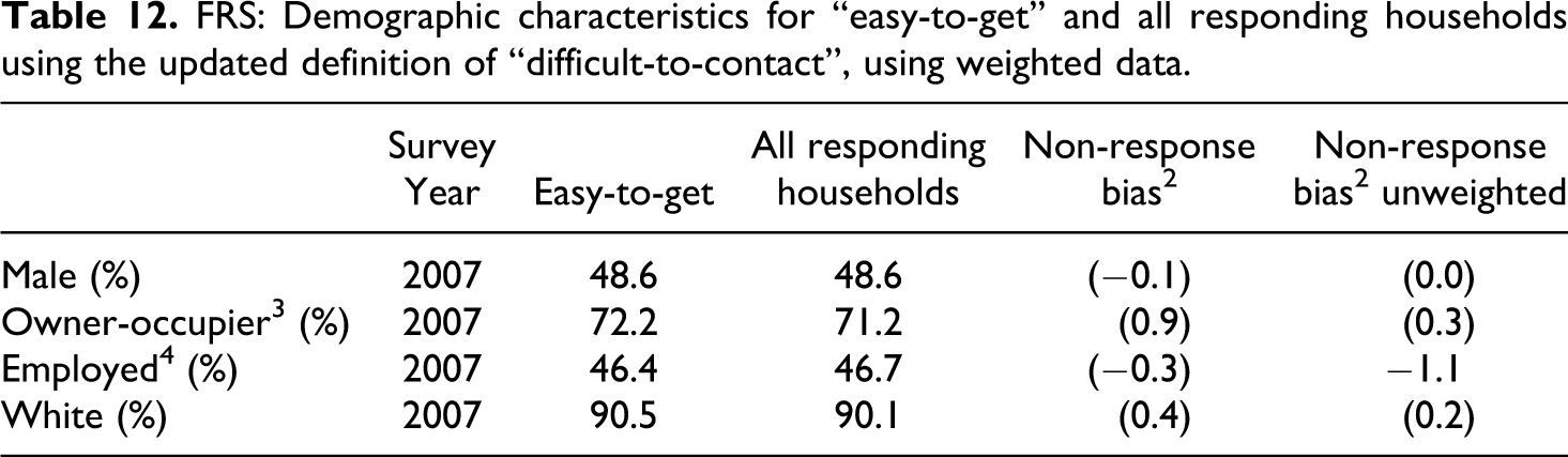
Tables 11 and 12 present weighted estimates for demographic variables and estimates of the marginal residual non-response bias, that is the difference between the two weighted estimates. Presented alongside are the estimates of marginal non-response bias using unweighted data. Due to space restrictions, results are presented only for HSE and FRS, though the results for all three surveys are summarised in the text. In both the HSE and the BSAS, the estimates of marginal non-response bias after weighting are generally smaller in magnitude than the estimates of marginal non-response bias from the unweighted data (the exceptions are percentage of males in the HSE in both 2006 and 2007, and the percentage of owner occupiers in the HSE 2007 and the BSAS 2006). For the FRS, the bias associated with three of the four demographic variables has increased in magnitude, but none of these differences are now significant.
HSE: Demographic characteristics for “easy-to-get” and all responding households using the updated definition of “difficult-to-contact”, using weighted data.
FRS: Demographic characteristics for “easy-to-get” and all responding households using the updated definition of “difficult-to-contact”, using weighted data.
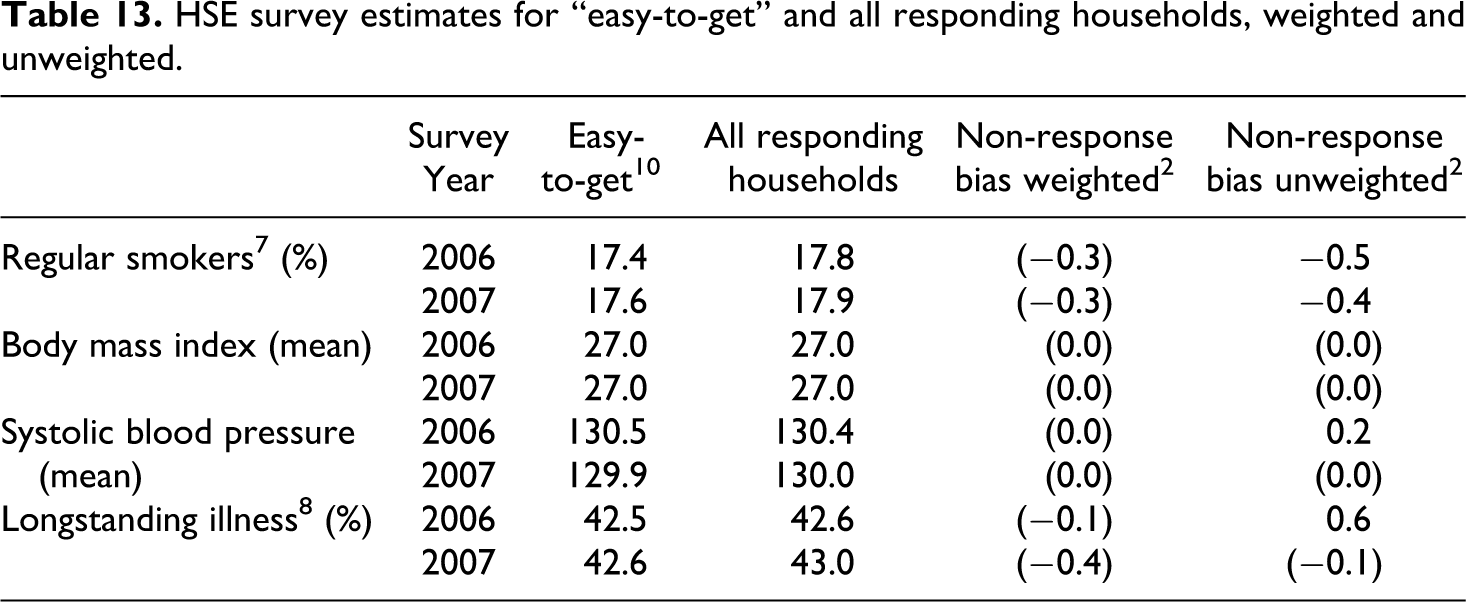
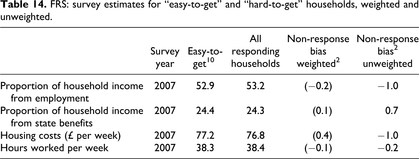
The findings for demographic variables are broadly replicated for the key survey variables for both HSE and FRS, but not for BSAS. The HSE estimates of marginal non-response bias after weighting are all smaller in magnitude than the unweighted estimates except for longstanding illness in 2007 (Table 13). After weighting, none of the estimates of marginal non-response bias remain significant. This is also true for the FRS: all of the biases in survey estimates are smaller in magnitude and no longer significant using the weighted data (Table 14). On the other hand, the non-response bias remaining for the BSAS weighted survey estimates are often larger in magnitude than the non-response bias found when using unweighted data (results not shown due to space restrictions). This is true for 13 of the 15 survey estimates in the BSAS 2007, and for three of the weighted survey estimates in the BSAS 2006 (although most are still not significant).
HSE survey estimates for “easy-to-get” and all responding households, weighted and unweighted.
FRS: survey estimates for “easy-to-get” and “hard-to-get” households, weighted and unweighted.
These results slightly weaken the case for investing in extended interviewer efforts. The findings suggest that appropriate weighting can remove much of the marginal non-response bias that would otherwise be removed by extended field efforts. However, the extent differs between variables. Broadly speaking, we find that weighting corrects for the marginal non-response in the case of health variables (with the exception of smoking behaviour), income and expenditure variables and demographic variables (with the exception of housing tenure), but not for attitudinal variables.
Conclusion
A number of important conclusions can be drawn from the analyses presented in this paper. There has been a substantial increase over the past decade in the proportion of households in Britain who are difficult to contact. This suggests that survey organisations must make more effort to achieve the same contact rates as a decade earlier. The cost of making contact is therefore increasing. Constant levels of effort will result in increasing non-contact rates. Changes in the relative amount (or effectiveness) of extended effort to make contact between surveys are also apparent. In 2006, for the first time, the HSE exceeded the BSAS with regards to the proportion of difficult to contact respondents. This finding reminds us that while difficulty of contact can be conceptualised as a population characteristic, survey-based indicators of difficulty of contact may be sensitive to survey-specific protocols and field procedures.
The proportion of reluctant households, that is those who initially refuse but take part after being reissued to another interviewer for refusal conversion, has more than tripled over a ten-year period for all three surveys. This finding may reflect a combination of increased reluctance in the population and increased propensity to attempt to convert initial refusals into respondents.
A decade after Lynn and Clarke (2002), demographic differences between “easy-to-contact” and “difficult-to-contact” households have changed little. Persons in “difficult-to-contact” households remain younger and much more likely to be employed than others, though we no longer find evidence of a difference in household size (Lynn and Clarke found that difficult-to-contact households were smaller, on average). Moreover, the proportion of employed respondents who live in hard-to-contact households has increased over time. Gender, home ownership and ethnicity still have only a weak association with ease of contact.
The demographic characteristics of reluctant respondents appear to have changed somewhat, however. Lynn and Clarke found mixed results regarding gender, with women more likely to be amongst the reluctant respondents for HSE, less likely for BSAS, and no gender difference for FRS. Now we find consistently across all three surveys that women are more likely to be reluctant respondents. We also find consistently that reluctant respondents are younger on average than other respondents, whereas Lynn and Clarke found no differences in mean age. Differences in terms of employment status also appear to have become more pronounced. Lynn and Clarke found no difference for HSE, a slightly greater tendency for reluctant respondents to be employed for FRS and only for BSAS a substantially greater tendency. Now we find a consistent and substantial tendency across all three surveys for reluctant respondents to be more likely to be employed. For both HSE and BSAS, reluctant respondents were previously more likely to be non-white, whereas this difference was no longer apparent in our study.
When looking at attitudinal measures, there are only small differences between “difficult-to-contact”, “reluctant”, and “easy-to-get” households, a finding consistent with Lynn and Clarke (2002). The health indicators and financial measures also largely replicate Lynn and Clarke’s findings. Members of “hard-to-get” households are more likely to have positive health indicators such as lower blood pressure, but are more likely to drink and smoke. And they have higher housing costs, receive a much larger proportion of their household income from employment and a much lower proportion from state benefits. These health and financial characteristics tend to be associated with younger respondents who are also more likely to be “hard-to-get”.
The overall picture, then, is that the role played by extended field efforts in reducing non-response bias appears to be at least as important as it was a decade earlier. Specifically, persons in “difficult-to-contact” households differ in characteristics from those who are “easy-to-get” just as much as they did a decade earlier, and are more prevalent, while “reluctant” respondents differ more clearly and consistently than they did before, and are considerably more prevalent.
We also investigated the sensitivity of the findings to the use of an improved measure of “difficult-to-contact”. Estimates of the effect of extended field efforts in reducing residual non-response bias using the new measure were similar for demographic estimates but fewer significant effects were apparent for the survey-specific estimates. Figure 2 demonstrates the reduction in bias in the percent employed as more visits are made to achieve first contact, and illustrates that a failure to pursue extended contact efforts is likely to bias any sample in terms of demographic characteristics. However, the hypothesis that extended efforts (that is, visits made after the fifth visit to obtain first contact with a household) reduce bias in key survey-specific estimates is weakened when we use this improved measure of “difficult-to-contact”.
A further extension in this paper was to assess the impact of extended efforts on estimates in the context of non-response adjustment weighting. The results suggest that the case for investing in extended interviewer efforts may be slightly weaker in situations where non-response weighting is a possibility. Appropriate weighting may remove much of the marginal non-response bias. In other words, although unweighted estimates are significantly affected by the extended efforts, weighted estimates are not affected to the same extent. However, the extent differs between variables. Broadly speaking we find that weighting corrects for the marginal non-response in the case of health variables (with the exception of smoking behaviour) and demographic variables (with the exception of housing tenure), but not for attitudinal variables. Nevertheless, even in the presence of weighting extended efforts appear to reduce non-response bias for some estimates. Furthermore, relying on weighting to achieve the same effects that might have been achieved by extended efforts is perhaps a risky strategy and will not always be possible as it depends on appropriate auxiliary data being available. We should perhaps conclude that the case for extended efforts is greater in situations where there is little or no relevant unit-level auxiliary information that can be used for weighting, for example from an informative sampling frame. The case may also depend on the survey topic. Our findings suggest a stronger case for surveys related to housing, smoking or attitudes than for surveys related to other health issues or to demography.
Footnotes
Acknowledgments
This research was funded by the ESRC Survey Design and Measurement Initiative via a research grant to Prof. Peter Lynn for the project “Understanding non-response and reducing non-response bias” (award RES-175-25-0005).