Sage Journals: Discover world-class research

Abstract

Key differences exist between individuals in terms of certain circadian-related parameters, such as intrinsic period and sensitivity to light. These variations can differentially impact circadian timing, leading to challenges in accurately implementing time-sensitive interventions. In this work, we parse out these effects by investigating the impact of parameters from a macroscopic model of human circadian rhythms on phase and amplitude outputs. Using in silico light data designed to mimic commonly studied schedules, we assess the impact of parameter variations on model outputs to gain insight into the different effects of these schedules. We show that parameter sensitivity is heavily modulated by the lighting routine that a person follows, with darkness and shift work schedules being the most sensitive. We develop a framework to measure overall sensitivity levels of the given light schedule and furthermore decompose the overall sensitivity into individual parameter contributions. Finally, we measure the ability of the model to extract parameters given light schedules with noise and show that key parameters like the circadian period can typically be recovered given known light history. This can inform future work on determining the key parameters to consider when personalizing a model and the lighting protocols to use when assessing interindividual variability.

Keywords

modeling tau shift work phenotype circadian rhythms

Circadian rhythms manage the timing of many physiological processes and impact a wide range of health outcomes and real-world applications. These include enabling individuals to better adjust to travel across time zones (Serkh and Forger, 2014; Christensen et al., 2020), allowing athletes to structure their daily schedule to perform at peak capacity (Thun et al., 2015), and assisting shift workers in minimizing their circadian disruption (Mohd Azmi et al., 2020; James et al., 2017). Shift work presents one of the most promising avenues for translational interventions, as working a shift work schedule has been associated with negative health outcomes, including gastrointestinal disorders, mood disorders, and cardiovascular disease (Costa, 1996; Warsame, 2014; Mosendane et al., 2008). Therefore, studying how the underlying physiological characteristics of individuals interact with various shift work schedules can have key real-world impacts in promoting health.

One of the primary manners in which the circadian rhythm of an individual becomes entrained to the typical 24-h cycle is through light input (Pittendrigh and Daan, 1976; Duffy and Wright, 2005; Duffy and Czeisler, 2009). While light is the dominant zeitgeber, research has also explored entrainment through non-photic stimuli such as activity levels, meal timing, and social interactions (Vetter and Scheer, 2017; Mistlberger and Skene, 2005; St Hilaire et al., 2007; Youngstedt et al., 2019). The recent advent of mobile technology allows for easy collection of light exposure and physiological measurements such as heart rate and activity, thus opening the door for large-scale modeling and analysis of wearable data. The prevalence of these data can enable personalized modeling in place of traditional one-size-fits-all approaches, thereby generating more accurate and effective circadian-based interventions. Thus, gaining a more precise comprehension of the factors that determine the circadian state of a given individual is a valuable area of research.

Mathematical models can generate predictions of human circadian state based on inputs of light (or, more recently, activity) time series. Classical versions of these models rely on a van der Pol oscillator framework, modulated by a light intensity input (Jewett and Kronauer, 1998; Jewett et al., 1999; Forger et al., 1999). These models are able to provide accurate assessments of circadian phase in humans, generating model phase predictions with mean errors on the order of 1 h for healthy populations when compared with commonly used phase markers such as laboratory dim light melatonin onset (DLMO) (Woelders et al., 2017; Huang et al., 2021). However, these models generally do not have a cohesive physiological basis, in that there are no direct biological analogues of all the parameters and variables studied.

More recently, a physiologically based model derived directly from modeling the individual neurons in the suprachiasmatic nucleus (SCN), the core circadian clock for mammals, has been developed (Hannay et al., 2019). While this model has been validated for both light and real-world activity data, a systematic evaluation of the effects of the parameter values has not yet been undertaken. Individuals likely vary substantially in several of the parameter values, such as intrinsic circadian period or light sensitivity (Stone et al., 2020; Phillips et al., 2019). For example, interindividual variations in circadian period can manifest in chronotype or sleep timing differences, and, together with light sensitivity, can impact the phase angle between melatonin onset and sleep (Phillips et al., 2010; Wright et al., 2005). Different sensitivities to evening light can additionally contribute to widely divergent DLMO timings and potentially negative health repercussions (Phillips et al., 2019). Hence, it is necessary to understand the impact of parameters on the model outputs in the context of the various light schedules that individuals may be following.

In this work, we analyze the effects of parameter variations on the circadian outputs generated by the physiologically based model. This sensitivity analysis is applied across a subset of common light schedules, and we see large-scale differences in model states depending on the interaction of the schedule and parameter. In particular, constant darkness and shift work schedules yield the highest overall parameter sensitivities, and the most impactful parameter across schedules is the intrinsic circadian period $τ$ . Using this framework, we can uncover parameter dependencies for individuals and focus on the most important factors for future model personalization. Furthermore, this analysis could help in better quantifying error bounds for DLMO prediction by showing the extent to which interindividual parameter differences can impact phase outputs for different light schedules.

Methods

We study the single population model for predicting circadian phase in humans. The single population model studied is given by the equations

\frac{d n}{d t} = 60 [α (L) (1 - n) - δ n],

α (L) = \frac{α_{0} L {(t)}^{p}}{L {(t)}^{p} + I_{0},}

B (t) = G (1 - n) α (L),

for the processing of the light input, and

\frac{d R}{d t} = - (D + γ) R + \frac{K}{2} \cos (β_{1}) R (1 - R^{4}) + L_{R} (R, ψ)

\frac{d ψ}{d t} = \frac{2 \cdot π}{τ} + \frac{K}{2} \sin (β_{1}) (1 + R^{4}) + L_{ψ} (R, ψ),

L_{R} (R, ψ) = \frac{A_{1}}{2} B (t) (1 - R^{4}) \cos (ψ + β_{L 1}) + \frac{A_{2}}{2} B (t) R (1 - R^{8}) \cos (2 ψ + β_{L 2}),

L_{ψ} (R, ψ) = σ B (t) - \frac{A_{1}}{2} B (t) (\frac{1}{R} + R^{3}) \sin (ψ + β_{L 1}) - \frac{A_{2}}{2} B (t) (1 + R^{8}) \sin (2 ψ + β_{L 2}),

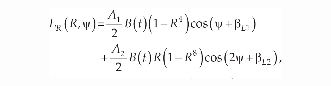
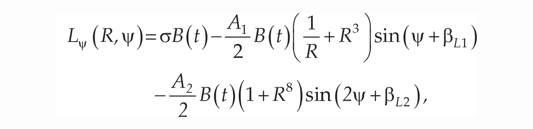
for the phase and amplitude equations (Hannay et al., 2019). In this macroscopic model, $R$ represents the collective amplitude of the oscillator population, $ψ$ corresponds to the mean collective phase of the oscillators, $L_{R}$ gives the impact of light on $R$ and $L_{ψ}$ likewise provides the impact of light on $ψ$ The parameters can also be understood physiologically, which allows for incorporation of more data sets and fine-tuning of coupling forces present in the SCN (Hannay et al., 2019). To extract circadian phase information, the collective phase at which $ψ = π$ is defined to correspond to the time of minimum core body temperature $(C B T_{\min})$

We adopt the default parameters values from the original paper (Hannay et al., 2019), wherein the parameters were fit based on light schedules and phase shifts available in existing experimental protocols (Khalsa et al., 2003; St Hilaire et al., 2012; Czeisler et al., 1989; Zeitzer et al., 2000). In this previous work, the parameters were estimated using a genetic global optimization algorithm and then the distributions of parameters around the optimal values were analyzed using a Markov Chain Monte Carlo (MCMC) algorithm (Hannay et al., 2019). We implement the ordinary differential equation (ODE) model and the rest of the analysis in Python. To determine initial conditions for $n, R$ and $ψ,$ we simulate the model once for a given number of days (typically 1 week) starting with arbitrary initial conditions and then take the final state value as the new initial condition; this process is repeated until the initial conditions converge or 50 iterations of this process have occurred. This process for initial condition determination is performed independently for each of the light schedules, unless otherwise specified.

In terms of parameter interpretations, we provide a brief summary based on previous work (Hannay et al., 2019; St Hilaire et al., 2007; Hannay, n.d.; Kronauer et al., 1999). In particular, the parameter $τ$ is the intrinsic circadian period, typically close to 24 h in duration when the shear parameter $β_{1} = 0$ (Guo et al., 2020; Montbrió and Pazó, 2011). For $β_{1}$ nonzero, the period of the oscillator is also amplitude-dependent. $K$ represents the averaged coupling strength between oscillators in the SCN; $γ$ controls the dispersion of the natural frequencies of the oscillators; $D$ represents the noise strength (set to zero here); $A_{1}$ $A_{2}$ $β_{L 1}$ $β_{L 2}$ and $σ$ determine the form of the phase response curve of neurons to light pulses and the entrainment angle of the model; $G$ is a scaling factor for the light drive onto the circadian pacemaker; $α_{0}$ is a scaling factor for the forward rate constant (i.e., the rate at which elements transition from the ready to used state); $δ$ is the rate at which elements move from the used to ready state based on the light stimulus; $p$ is an exponent on the light input according to the Process L formalism; and $I_{0}$ scales the light intensity according to the Process L formalism (Kronauer et al., 1999). For more details on the derivation of the model and parameter interpretation, see the previously published work (Hannay et al., 2019; Kronauer et al., 1999).

We examine 6 synthetic light schedules for the majority of the analysis, given below:

A regular light schedule, given by 16 h of light starting at 8 am and followed by 8 h of darkness, repeating on a daily basis. We abbreviate this schedule as RL.

A first shift work light schedule, consisting of 5 days working a night shift followed by 2 days off. The days working a night shift are defined by waking up at 4 pm followed by 16 h of light, while the days off the night shift consist of the same schedule with a 9-am wakeup. We abbreviate this schedule as SW.

A second shift work schedule, defined by three 12-h night shifts (with a wakeup time of 7 pm and a 16-h workday) followed by 4 days on a regular light schedule (with a wakeup time of 7 am and a 16-h workday). We abbreviate this schedule as SW312.

A social jet lag schedule, wherein light exposure occurs 7 to 12 am for 5 days a week (e.g., Monday-Friday) and occurs between 11 and 2 am two days a week (e.g., Saturday and Sunday). We abbreviate this schedule as SJL.

A slam shift schedule, in which light exposure starts at 8 am and lasts for 16 h five days a week, and then shifts to 4 pm (lasting 16 h still) for 2 days a week. We abbreviate this schedule as SS.

A constant routine schedule, where light exposure is always constant. We abbreviate this schedule as Dark when light is zero, and CR when light may be nonzero.

For light intensity, we set the default to be L = 979 lux, based on previous work assessing typical daytime light levels (Wright et al., 2013). The exception is the constant routine schedule, where the default is a constant darkness schedule, with L = 0 lux (Figure 1b). Since this may be a higher-than-expected constant light intensity level, particularly in the evening, we also study sensitivity results under lower light levels. In particular, we vary the constant light intensity over the range of 0-950 lux in intervals of 50 lux and compare the overall parameter effects (Figure 4) and individual parameter contributions (Suppl. Fig. S3).

As a first assessment of parameter sensitivity, we compute the Hessian matrix of a loss function. This loss is a function of a scaling vector $λ$ applied to a set of parameter values $θ$ defined by taking a mean distance measurement between the state values $s_{θ}$ with the given set of parameter values $θ$ and the state values $s_{θ^{*}}$ with the original/default parameter values $θ^{*}$ The parameters $s_{θ}$ are specified by the amplitude $R_{θ}$ and phase $ψ_{θ}$ outputs, where $R_{θ}, ψ_{θ} \in ℝ^{N}$ for $N$ the number of data points. Specifically, we define a loss function $L (λ) = (1 / N) \sum_{n = 1}^{N} ({(x_{n}^{(1)} - x_{n}^{(2)})}^{2} + {(y_{n}^{(1)} - y_{n}^{(2)})}^{2})$ where $x^{(1)} = R_{θ} \cos (ψ_{θ}), x^{(2)} = R_{θ^{*}} \cos (ψ_{θ^{*}}), y^{(1)} = R_{θ} \sin (ψ_{θ}), y^{(2)} = R_{θ^{*}} \sin (ψ_{θ^{*}})$ and

parameters $θ = λ \cdot θ^{*}$ for $θ^{*}$ representing the default parameter values. So, at $θ = θ^{*}$ (the default parameters), we have $λ = λ^{*} = \vec{1}$

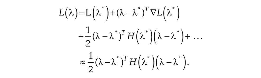
Note that by construction $L (λ^{*}) = 0$ and $\nabla L (λ^{*}) = 0$ Defining $H$ as the Hessian matrix of $L$ we can expand this loss function around the default parameter values as

\begin{array}{l} L (λ) = L (λ^{*}) + {(λ - λ^{*})}^{T} \nabla L (λ^{*}) + \frac{1}{2} {(λ - λ^{*})}^{T} H (λ^{*}) (λ - λ^{*}) + \dots \\ \approx \frac{1}{2} {(λ - λ^{*})}^{T} H (λ^{*}) (λ - λ^{*}) . \end{array}

We can compute the Hessian matrix at the default parameter values, $H (λ^{*})$ via the Jax library in Python (Bradbury et al., 2018). The Hessian serves as a second-order approximation for the contours of constant loss function behavior around the default parameter values, with the eigenvalues corresponding to the lengths of the ellipsoids (a stretch factor) and the eigenvectors denoting the direction of the axes. We then define several sensitivity-related metrics based on the form of this Hessian matrix: for overall sensitivity, we compute the Frobenius norm. For the effects of the individual parameter values, we compute the magnitude of the components of the eigenvector associated with the largest eigenvalue of the Hessian matrix.

In addition, we systematically vary parameters over realistic ranges to more easily assess the impact of each parameter on the resultant model states visually. Specifically, we use parameter distributions determined from MCMC simulations in previous work to define reasonable sets of parameter values (Hannay et al., 2019). For the cases in which this distribution is available, we draw values from the 5th to 95th percentile, typically in increments of 10 percentiles, where the percentile values are shifted so that the 50th percentile aligns with the default parameter value. Otherwise, we vary each parameter from 91% to 109% of their default value, typically in increments of 2%, while again holding the other parameters fixed. Note that the distributions are available for all of the parameters except for $G$ and $δ$ that is, these 2 parameters are varied by the percentages of their default values, while all others are drawn from the percentiles of the distribution. After this, we examine the changes of output (i.e., amplitude $R$ and phase $ψ$ in the form $R \cos (ψ)$ time series across the parameter values.

To measure the extent to which we can determine true parameters in the presence of noisy light or activity inputs, we perform a parameter recovery analysis. Specifically, we simulate the model with perturbed parameter values (systematically varied) and perfectly known (i.e., exact) light levels, storing the resulting model outputs. We vary the parameters in a similar way to the previous analysis, either drawing from the parameter distributions when available or perturbing between 91% and 109% of their default values (here in increments of 1%). We additionally simulate the model with noisy light schedules and known parameter values, also drawn from distributions or perturbed over the same range. This again generates phase and amplitude model outputs, which we store. After comparing the results from the noisy and non-noisy light schedule simulations, we extract the perturbed parameter (with exact light) values that generate the closest result to the given noisy simulation. We determine this based on the $R \cos (ψ)$ -based norm difference in model outputs, which we call the recovery error here, given as

L = \frac{1}{N} \sum_{n = 1}^{N} ({(x_{n}^{(1)} - x_{n}^{(2)})}^{2} + {(y_{n}^{(1)} - y_{n}^{(2)})}^{2})

where $x^{(1)} = R_{θ_{p}} \cos (ψ_{θ_{p}}), x^{(2)} = R_{θ^{*}} \cos (ψ_{θ^{*}}), y^{(1)} = R_{θ_{p}} \sin (ψ_{θ_{p}}), y^{(2)} = R_{θ^{*}} \sin (ψ_{θ^{*}}),$ and parameter $θ_{p}$ represents the perturbed parameters and parameter $θ^{*}$ represents the default or known parameter values. From this, we can assess how closely the perturbed parameter results (with exact light) match those of the known parameters (with noisy light). We compute an overall difference in recovery error metric for each parameter, by determining the average recovery error $L_{m}$ for all matching percentiles of the given parameter (i.e., the average recovery error between states generated by noisy light with nth percentile parameters and states generated by exact light with nth percentile parameters) and the average recover error $L_{n m}$ for all non-matching percentiles of the given parameter (i.e., the average recovery error between states generated by noisy light with nth percentile parameters and states generated by exact light with non-nth percentile parameters). We then take $L_{n m} - L_{m}$ as the difference in recovery error. If a parameter is often recovered correctly, we would expect a higher recovery error for non-matching parameter percentiles than for matching parameter percentiles, and thus a higher value of this measurement. And a value less than or equal to zero would suggest an overall inability to recover the particular parameter. This analysis allows us to study the extent to which default and non-default parameter values can be determined from the model, in the presence of various light schedules and noise. Indeed, the parameter recovery analysis will give us insight into the degree that noise in the light schedules can be mistaken for differences in the parameters. Code to run the analyses in this article is available at https://github.com/mayercl/sensitivity-analysis-.

Results

After simulating the model (see Methods) with each of the 6 synthetic light schedules (Figure 1a) as input, we examine the changes in model output determined by altering particular parameter values (Figure 1b) or the Hessian-based notions of sensitivity (e.g., Figure 2). The model trajectory with default parameter values is shown in blue, and trajectories with perturbed parameters are shown in gray. We simulate all of the in silico schedules for 7 days (Figure 1a).

Figure 1.

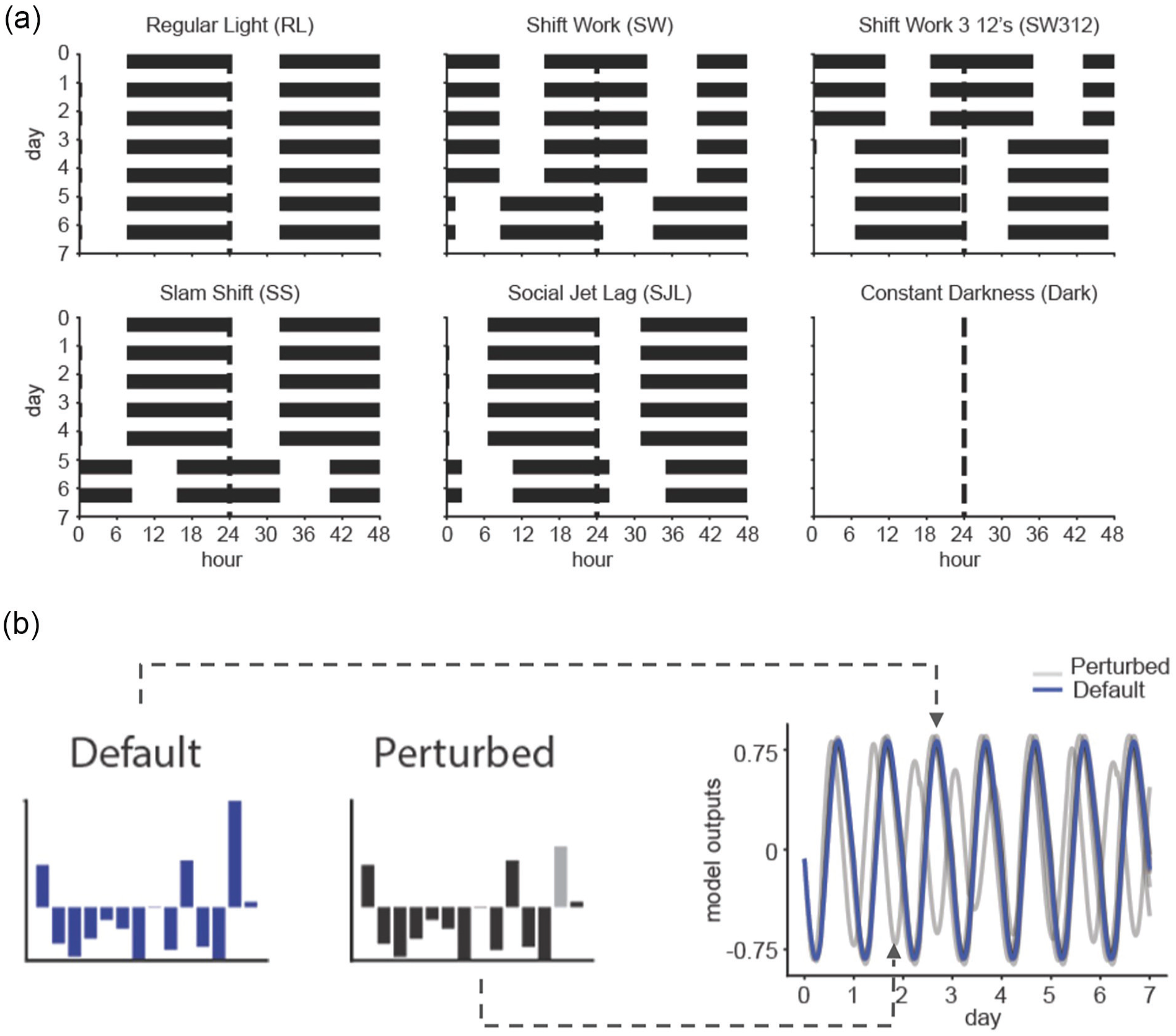
Methodology: Schematic and light schedules. Schematic of the process: the Hannay model is simulated with the 6 different light schedules (actograms, a) as input. Using this framework, we are able to assess the impact of the parameters on the model outputs (b). This can be done by computing the Hessian matrix (see Methods) and by examining the perturbed trajectories of the model (b). The default and perturbed parameter values shown in (b) are not to scale. To generate the perturbed model outputs (gray curves) in (b), we vary the parameters from their default values (e.g., the gray bar in (b), left, corresponds to a particular gray curve in (b), right).

Figure 2.

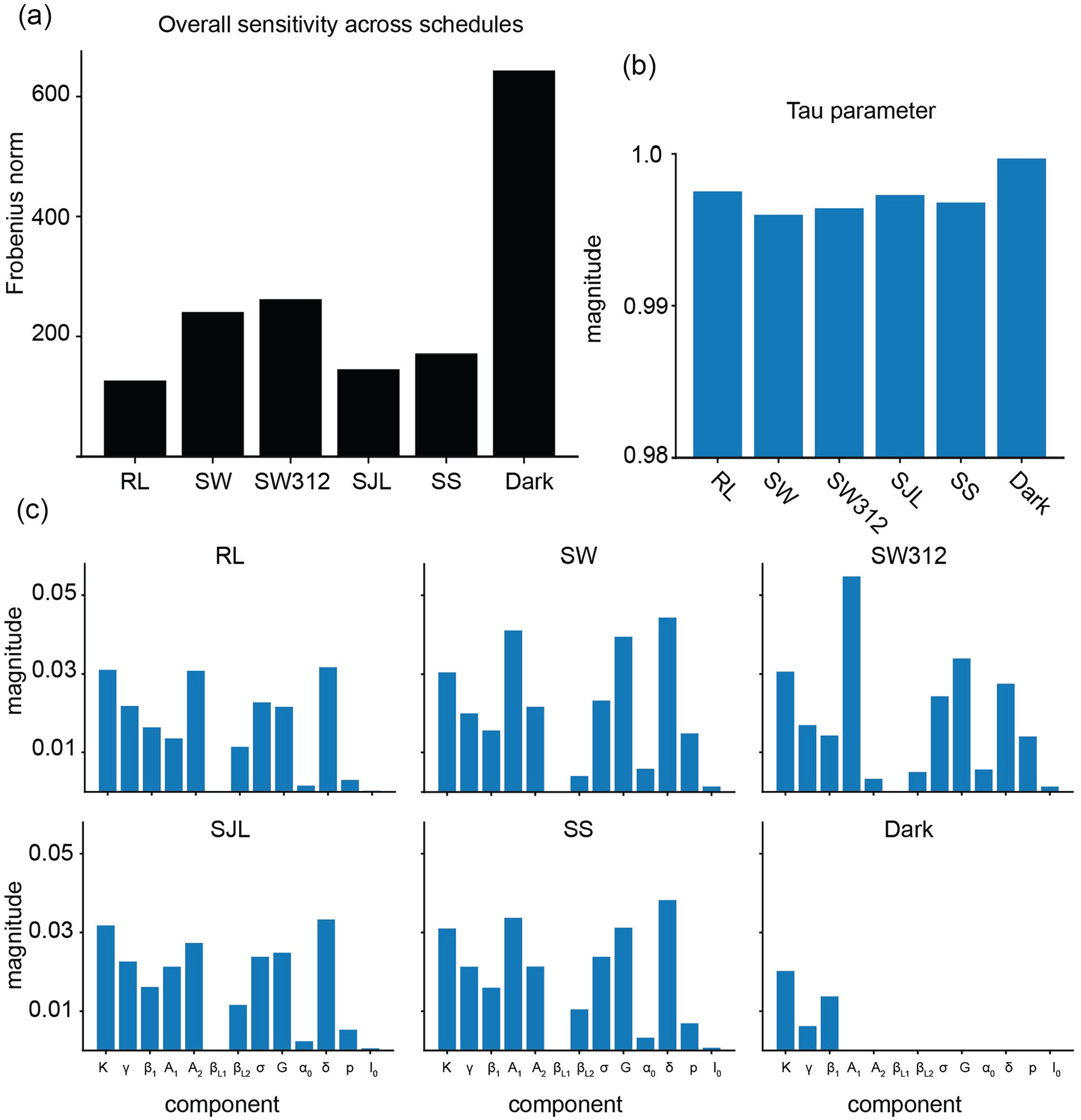
Overall and individual-parameter Hessian-based sensitivity across light schedules. (a): The overall sensitivity for each of the 6 light schedules computed as the Frobenius norm of the Hessian. (b): The magnitude of the first component of the principal eigenvector of the Hessian. The light schedule abbreviations are as follows: RL means regular light schedule, SW means shift work, SW312 means shift work with three 12-h shifts, SJL means social jet lag, SS means slam shift, and dark means constant darkness. The 14 parameter values, in order, are given by $τ$ $K$ $γ$ $β_{1}$ $A_{1}$ $A_{2}$ $β_{L 1}$ $β_{L 2}$ $σ$ , $G$ $α_{0}$ $δ$ $p$ and $I_{0}$ For visualization purposes, the first component (corresponding to the $τ$ parameter) is plotted separately, and the remaining 6 plots in (c) for the individual light schedules exclude this first component.

The Frobenius norm of the Hessian matrix, serving as a measure of total sensitivity, varies from 643.60 for the constant darkness schedule to 126.93 for the regular light schedule (Figure 2a). The shift work with three 12-h shifts schedule (SW312) has the second largest Frobenius norm of 262.36, followed by the shift work schedule (240.96), the slam shift schedule (171.52), and the social jet lag schedule (145.83). The principal eigenvector components also vary across schedules: while the largest parameter component corresponds to $τ$ for all the schedules, the second largest is $δ$ for the regular, shift work, social jet lag, and slam shift schedules. The second largest parameter component is $A_{1}$ for the shift work with three 12-h shifts schedule, and $K$ for the constant darkness schedule (Figure 2c). The smallest in magnitude component is $β_{L 1}$ for all of the non-dark schedules. For constant darkness, only the first 4 parameter values $(τ$ $K$ $γ$ $β_{1}$ contribute to this sensitivity metric, as light input is zero.

While the initial conditions used in Figure 2 are generated via looping until convergence from the individual schedule, we tested other initial condition approaches. Under the assumption that a regular light schedule precedes each of the 6 individual weeks, we can generate new initial conditions and compute the Hessian-based results. In this case, we see that constant darkness remains the most sensitive, followed by shift work, shift work with three 12-h shifts, slam shift, social jet lag, and regular light (Suppl. Fig. S1B). Furthermore, we show the dependence of the Hessian norm sensitivity on more general initial conditions for $R$ and $ψ$ from the unit circle, for the 6 schedules of interest (Suppl. Fig. S1C).

In addition, we show the eigenvalues of the Hessian in Supplementary Figure S2.

Amplitude and phase results after performing one-at-a-time parameter perturbations (where parameters are perturbed by drawing from available distributions when available; see Methods) are shown for the 6 light schedules of interest in Figure 3a (default parameters: red, perturbed parameters: gray). Using the loss function $L (λ)$ defined in Methods, we can compute this function for each parameter perturbation and light schedule. If we average this function across parameter perturbations, parameters, and light schedules, we see that the constant darkness schedule has the highest value of this norm difference (0.0233), followed by the shift work with three 12-h shifts schedule (0.0107), the shift work schedule (0.0105), the slam shift schedule (0.0080), the social jet lag schedule (0.0072), and the regular light schedule (0.0065). We also break down the values of the loss function by parameter and schedule (Figure 3b). We see that for all schedules, the parameter $τ$ generally gives high loss values when perturbed (with mean norm difference loss values ranging from 0.05 to 0.20), as does the parameter $β_{1}$ (with mean norm difference values ranging from 0.038 to 0.13).

Figure 3.

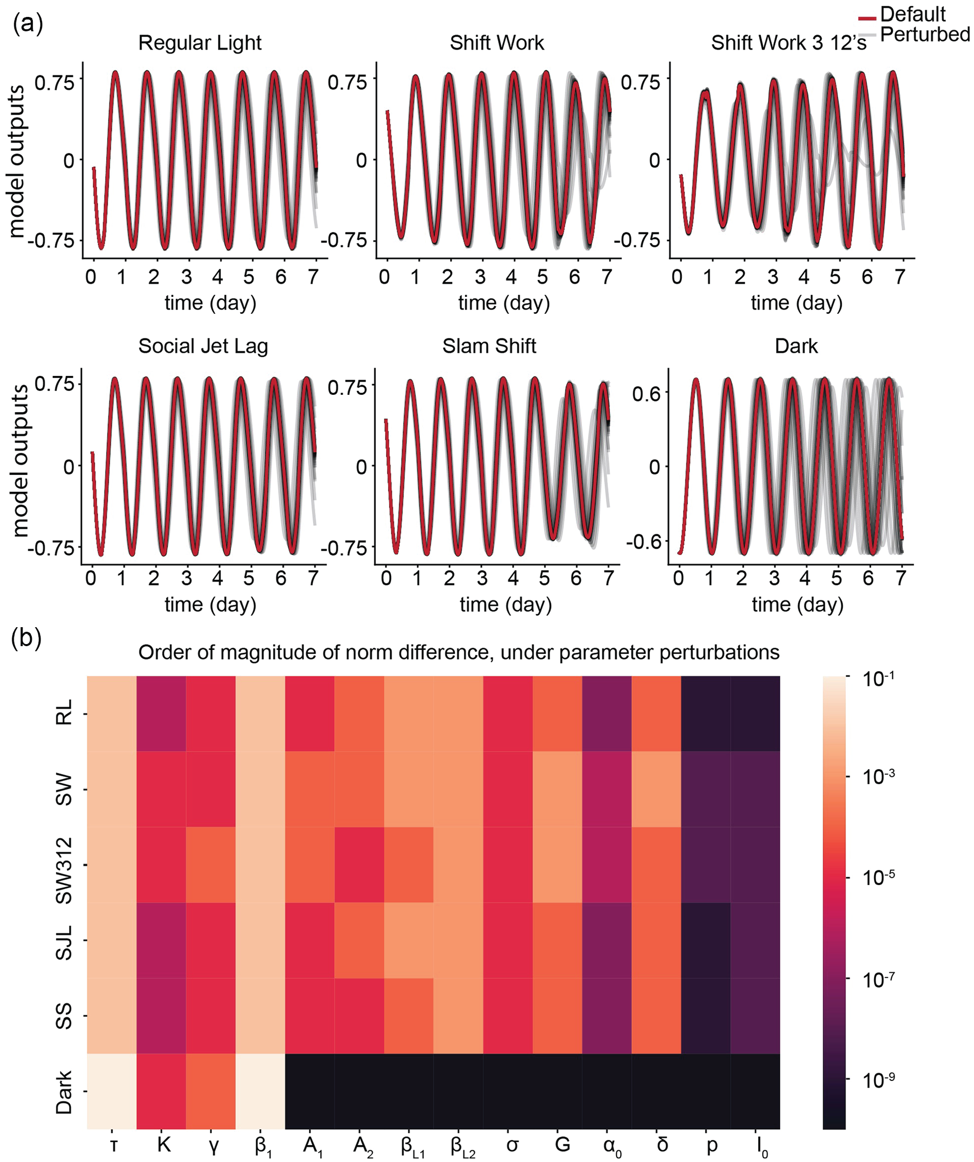
Parameter output schedule differences for 6 synthetic light schedules. We examine the differences in the model outputs for the 2 shift work schedules. (a): Model amplitude and phase (plotted as $R \cos (ψ))$ comparison for the 6 schedules, over the course of 7 days. The time series with default parameters is plotted (red line), and then the parameters are each varied over the specified range (see Methods) and the results are plotted (gray lines). (b): Heatmap for the order of magnitude of the mean norm difference between the states defined with perturbed model parameters and states generated by default parameters, averaged across the perturbation levels. Orders of magnitude less than or equal to $10^{- 10}$ are binned together, in the darkest bins. Abbreviations: RL = regular light; SW = shift work; SW312 = shift work with three 12-h shifts; SJL = social jet lag; SS = slam shift; dark = constant darkness.

In addition, using this perturbation approach, we can quantify changes in the DLMO prediction from the model. For all of the light schedules, the 2 parameters that give the largest variation in DLMO prediction (as measured by the circular standard deviation across parameter perturbations) are again $τ$ and $β_{1}$ For regular light, the DLMO standard deviations under $τ$ and $β_{1}$ perturbations are 1.148 and 1.259 h, respectively. For shift work, they are 1.323 and 1.357 h; for shift work with three 12-h shifts, they are 1.400 and 1.158 h; for social jet lag, they are 1.658 and 2.005 h; for slam shift, they are 1.172 and 1.827 h; and for constant darkness, they are 1.821 and 1.868 h, respectively. The other parameters have much smaller effects on DLMO variations (see Suppl. Tab. S1 for details). Note that these measurements do not include the parameter effects on amplitude.

In Figure 4, we show the norm difference for the Hessian-based overall sensitivity results as a function of lower values of light intensity (varying from 0 to 950 lux in increments of 50 lux). As the light intensity increases, the norm of the Hessian consistently decreases across the regular light, shift work, social jet lag, and slam shift schedules. However, for the shift work with three 12-h shifts and the constant routine schedule, this metric shows more fluctuations across intensity values. The order of the most impacted schedule is also generally consistent across light intensities, with constant routine always having the highest norm of the Hessian. As in Figure 2, the next schedule in terms of this overall sensitivity metric is typically shift work with three 12-h shifts; however, shift work has a slightly higher norm of the Hessian for 100 and 150 lux (422.28 vs 395.71 for 100 lux, and 366.26 versus 331.12 for 150 lux for shift work and shift work with three 12-h shifts, respectively). The schedule with the lowest Hessian norm is always regular light, with values ranging from 430.93 at 50 lux to 127.30 at 950 lux. We further plot the magnitude of the individual parameter components for the schedules and different lighting intensities in Supplementary Figure S3.

Figure 4.

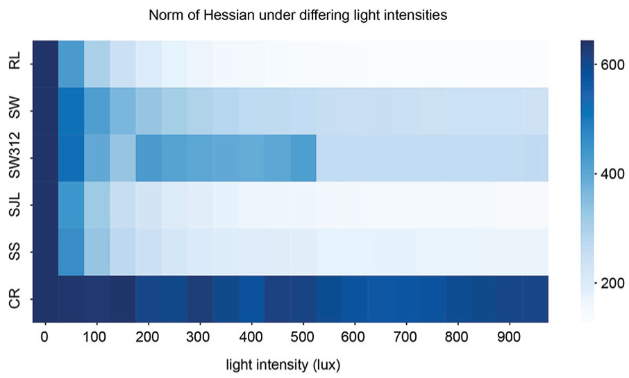
Overall sensitivity under differing light intensities. We vary the light intensity from 0 to 950 lux, in increments of 50 lux, and examine the impact on the overall sensitivity across the 6 schedules of regular light (RL), shift work (SW), shift work with three 12-h shifts (SW312), social jet lag (SJL), slam shift (SS), and constant routine (CR). Darker blue colors denote higher values for the norm of the Hessian, given the particular light schedule and intensity combination.

To determine the extent to which parameters can be determined in the presence of noisy light schedules, we perform a parameter recovery analysis. In Figure 5a and 5b, we determine the parameter percentile or perturbation index where the minimum recovery error occurs. We then plot the number of indices between this index and the theoretical best matching index (at a percentile of 50% or a perturbation of 1.0, meaning no change in parameters), for each light schedule and parameter values. We used a fixed noise level (random noise with standard deviation of 100) in the light schedules, in all places except Figure 5a (random noise with standard deviation of 10). The parameters most frequently recovered across the light schedules are $β_{1}$ and $τ$ In the low noise level case (Figure 5a), all parameters had a high degree of recoverability, except for the constant darkness schedule and $I_{0}$ in the shift work with three 12-h shifts, social jet lag, or slam shift schedules. In particular, parameters $τ, γ, β_{1}, β_{L 1}, β_{L 2}, G$ and $δ$ were all exactly correctly recovered across all schedules except constant darkness. In the high noise level case (Figure 5b), $β_{1}$ was correctly recovered or one index away from being correctly recovered across all the light schedules except for constant darkness (with noise injected), and $τ$ was within 3 or less indices of being correctly recovered for all of the schedules except for constant darkness (with noise injected). However, clearly many parameters (such as $K$ and $A_{1}$ cannot be well recovered for the given light schedules and noise level (see Figure 5b).

Figure 5.

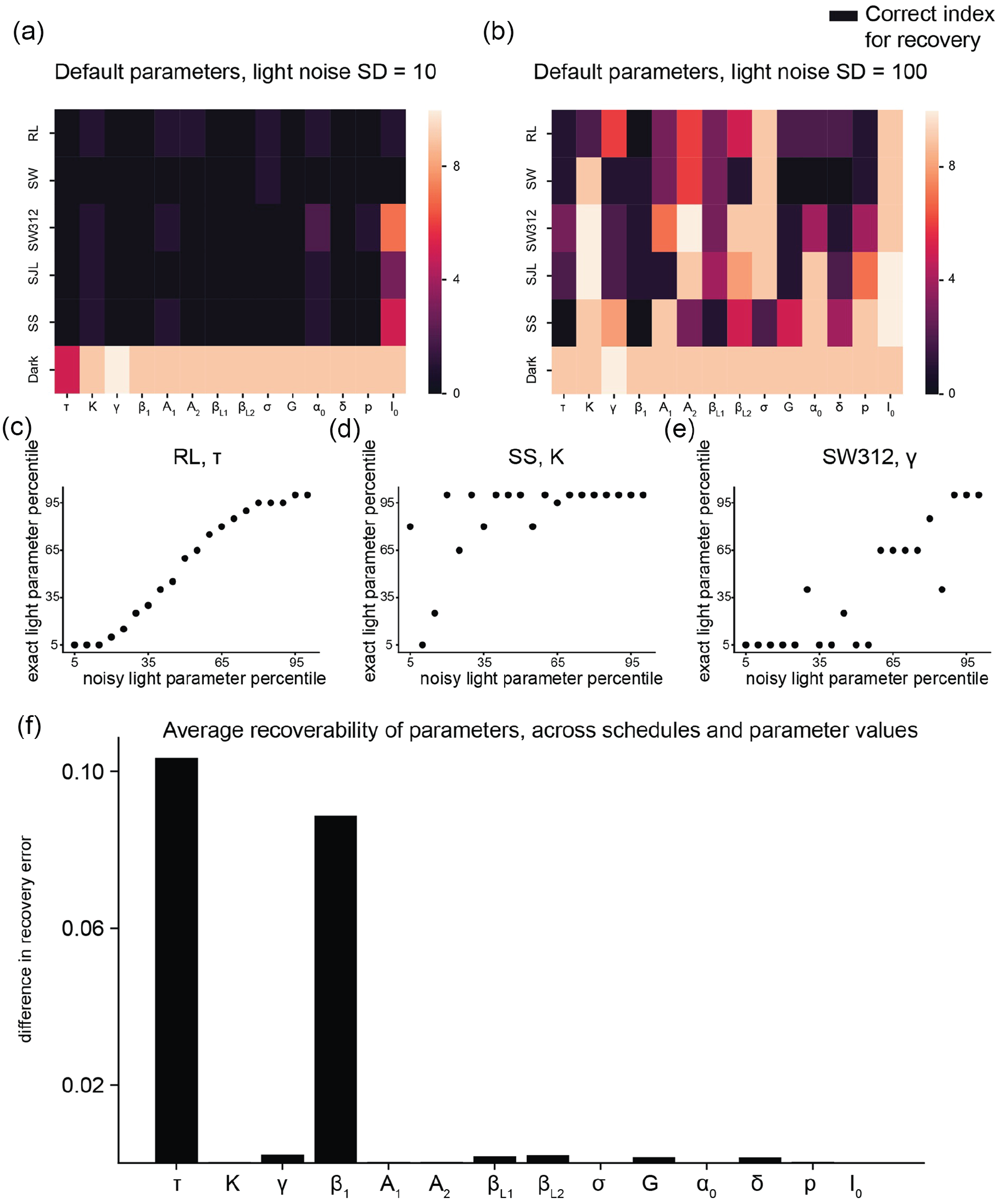
Parameter recovery. (a-b): We show the results of a parameter recovery analysis: after simulating with default parameters and noisy light schedules and perturbed parameters and fixed light schedules, we examine the degree to which the correct parameters can be recovered via a matching procedure (see Methods). The 6 schedules are shown on the vertical axis, and the parameters on the horizontal axis: the heatmap is colored by the absolute value of the distance from the correct recovery index, with an index of 0 corresponding to the correct parameter being recovered. In (a), we consider a low noise level in the light (SD = 10 lux), and we consider a higher noise level (SD = 100 lux) in (b). (c-e): We show examples of recovery error for various parameter and light schedule combinations. Here we consider non-default parameters with noisy light, and for each non-default parameter perturbation with noisy light (vertical axis), we compute the parameter percentile with exact light that generates the lowest recovery error. A perfect parameter recovery at all parameter percentiles would correspond to the diagonal line y = x. We plot this metric for 3 example parameter and light schedule combinations: regular light with $τ$ in (c), slam shift with $K$ in (d), and shift work with three 12-h shifts with $γ$ in (e). (f): We compute an aggregate recoverability score for each of the parameters, averaged across parameter perturbations and light schedules. In particular, we compute the recovery error under matching parameter percentiles and subtract this from the recovery error under non-matching parameter percentiles. See Methods for details. Abbreviations: RL = regular light; SW = shift work; SW312 = shift work with three 12-h shifts; SJL = social jet lag; SS = slam shift; dark = constant darkness.

In Figure 5c-5e, we show specific examples of what the differences in the recovery can look like for the higher light noise case. Given a particular parameter and parameter percentile under the noisy light levels, we plot the parameter percentile under exact light levels that provides the minimum recovery error. So if recovery is perfect, noisy light 5th parameter percentile will match with exact light 5th parameter percentile, noisy light 10th parameter percentile will match with exact light 10th parameter percentile, and so on until we get the diagonal line. In Figure 5c, we see an example relatively close to this perfect recovery case with $τ$ and a regular light schedule. However, many of the other parameters and light schedule combinations do not follow this recoverable pattern (see Figure 5d and 5e for examples). We also compute an overall measurement of recovery, by parameter value (Figure 5f). This measurement involves computing an average difference between matching parameter percentiles and non-matching parameter percentiles; see Methods for details. By this measurement, averaging across light schedules and parameter percentiles, we see high recoverability for τ $β_{1}$ and $τ$ in particular (with values of 0.103 for $β_{1}$ and 0.089 for $γ$ The other parameter has a much lower difference in recovery errors, with the next 2 largest values being 0.0023 and 0.0020 for $β_{L 2}$ and $p$ respectively.

Discussion

Examining the interactions between model parameters and light schedules can improve our understanding of model personalization and guide future interventions. Indeed, parameter effects and interindividual differences in circadian models have been shown to impact important factors such as phase prediction, chronotype, and effectiveness of social scheduling alterations (Stone et al., 2020; Phillips et al., 2010; Skeldon et al., 2017). Interindividual variations in intrinsic circadian period and light sensitivity have been of particular interest and have been shown to relate to significant changes in DLMO and detrimental health outcomes (Phillips et al., 2019; Stone et al., 2020). In this work, we study several measures of parameter impact in a physiologically derived model for human circadian rhythms and show that key interactions between light schedules and model parameters can drive large variations in phase and amplitude predictions. Indeed, our work shows that the interindividual differences in the intrinsic circadian period can have important repercussions for the model outputs and phase predictions. While previous work has also highlighted the important role of light sensitivity, we find that parameters relating to this sensitivity (e.g., $τ$ generally do not play as prominent a role in this analysis. It could be the case that individuals differ more significantly in lighting sensitivity than we are capturing in our modeling. Future work to fit these parameters in a personalized manner, or based on data across populations, could help to elucidate this point.

When we take a Hessian-based view of sensitivity, we see large differences depending on the particular lighting schedule of the individual. For example, the constant darkness and shift work schedules are the most sensitive to parameter perturbations overall in terms of the Frobenius norm of the Hessian. This means that parameters are particularly relevant for individuals on these schedules and can lead to divergent outcomes overall. It is worth noting that 3 of the most irregular schedules (shift work, shift work with three 12-h shifts, and slam shift) have some of the highest overall sensitivity values both at the chosen default lux value and across variations in light intensity, suggesting that the inconsistent nature of these schedules amplifies differences between individuals. The sensitivity of shift work schedules could contribute to challenges when using this or similar models to predict phase markers in shift worker populations, as lack of parameter personalization may be particularly impactful for these schedules.

Similarly, constant darkness obviously does not generate entraining patterns. Even though many of the light-related parameter variations do not impact the constant darkness results, the lack of entraining signal likely makes this schedule very sensitive to the parameters that do impact it (especially $τ$ which plays a large role in all the schedules). On the other hand, the regular light and social jet lag schedules have the lowest sensitivity values overall. The lower sensitivity for these 2 schedules is perhaps not surprising, as we hypothesize that more consistent schedules facilitate entrainment and thereby suppress the effect of interindividual differences. This idea may be consistent with the light intensity results as well, since we see that higher intensities (and thus more well-defined schedules) correspond to lower parameter sensitivity measurements. Future work is needed to examine further variations on these schedules, to better inform research that studies the effects of shift work on outcome variables.

Interestingly, the initial conditions of the model play a significant role in the Hessian-based sensitivity results. Here, we have focused on an initial condition approach where we loop until convergence for each individual schedule, a method that matches the assumption that individuals maintain their specific schedule on a weekly basis. This is not the only possibility, however, as some individuals likely switch from one schedule to another on an inter- or intra-weekly basis. We also investigated sensitivity results under the assumption that individuals were on a regular light schedule (or various other initial phase and amplitude values) before embarking on their particular schedule, and we see alterations to the results (see Suppl. Fig. S1). The large effect of initial conditions speaks to the importance of accurately determining these when generating phase predictions using the model, which could be facilitated by wearable data collection over longer time intervals.

In terms of the individual parameter sensitivity, the constant darkness schedule only depends on the first 4 parameter values $K$ $γ$ $β_{1}$ and $τ$ as the other parameters involve the light input equation at some stage. In terms of the parameter recovery analysis, it follows that the majority of the parameters will not be able to be determined from a constant darkness routine. While constant schedules have often been used in the circadian literature to control for external stimuli, this result highlights the fact that for the purposes of fitting light-sensitive parameters, schedules other than constant darkness are needed. Interestingly, the constant darkness schedule still has a larger overall sensitivity than all of the non-darkness schedules, despite only depending on a smaller subset of the parameters. This is likely due to the impact of the $τ$ parameter, for all schedules but particularly for constant darkness (in which no external signals can modulate intrinsic period changes). Overall, these results suggest the impact of τ $β_{1}, K, A_{1}, A_{2},$ in determining the model states, and hence its role as an important parameter to consider in future personalization. Other parameters of import depend to a larger degree on the specific methodology and include $δ$ and $τ$ Parameter components from the Hessian-based analysis vary across light intensities: for example, while $σ, δ$ has a relatively large magnitude across all the lighting conditions, this decreases as light levels rise. This may further support the idea that strong entraining signals mitigate the impact of interindividual parameter differences. However, the magnitude relating to certain parameters also increases with light intensity, particularly in parameters directly related to the light-processing portion of the model (e.g., $τ$ These results suggest that the relative importance of parameters vary to a degree based on both the light schedule and the intensity of light in the surrounding environment.

This work studies the sensitivity of parameters in a model for human circadian rhythms and does not consider the effects of sleep-wake regulation. Indeed, we know that there are bidirectional relationships between sleep-wake processes and circadian rhythmicity, and that sleep-wake regulation occurs via both the circadian system and the sleep homeostatic process (Skeldon et al., 2017; Phillips et al., 2010). Hence, while we assume that the schedules are fixed in this analysis, it is reasonable to expect that the physiological changes and interindividual differences that we capture via the parameter perturbations could impact the sleep schedules themselves. Future work could incorporate this model of the circadian system in conjunction with sleep homeostasis to further analyze parameter effects.

In the parameter recovery analysis, we see that some of the key parameters such as $β_{1}$ could be recovered from the model simulations. In particular, $τ$ and $τ$ were the most frequently recovered parameters across light schedules, likely due to the large effect that period perturbations can have on the phase marker outputs. Indeed, $β_{1}$ controls the intrinsic period directly, while β₁ relates to how the period depends on the amplitude (Hannay et al., 2019). Many parameters could not be recovered, however, both in the constant darkness (where these parameters do not impact the resulting model states) and in the non-darkness schedules. We should note that clearly the light noise level (typically set to a standard deviation of 100 here) plays a large role in the extent to which the noisy light obscures the true values of the parameters as well. Recovery is much easier under less variance in the lighting schedule, as shown by the fact that we can accurately recover almost every parameter under a lower light noise level. Indeed, future work could explore the interactions between the light noise level and the parameter range in terms of determining successful recovery. Another factor to consider is the length of data; here the simulations occurred over 7 days for each schedule, but performing parameter recovery over different time spans could alter the results to some degree. While we chose 7 days as the shortest possible time span to capture weekday and weekend variations, future work could explore further variations on these schedules over longer durations.

Overall, this work enables us to gain a better understanding of how light schedules, initial conditions, and parameters interact to determine the model predictions. This knowledge can inform future work on parameter personalization, in that given a particular light schedule, we now have insight as to the expected effect of the parameters and which specific parameters to focus on when incorporating interindividual differences. Indeed, this work helps us quantify the impact that interindividual variations in both parameters and lighting routines can have on the circadian outcomes of individuals.

Supplemental Material

sj-docx-1-jbr-10.1177_07487304231176936 – Supplemental material for Impact of Light Schedules and Model Parameters on the Circadian Outcomes of Individuals

Supplemental material, sj-docx-1-jbr-10.1177_07487304231176936 for Impact of Light Schedules and Model Parameters on the Circadian Outcomes of Individuals by Caleb Mayer, Olivia Walch, Daniel B. Forger and Kevin Hannay in Journal of Biological Rhythms

Footnotes

Acknowledgements

The authors disclosed receipt of the following financial support for the research, authorship, and/or publication of this article: This work was supported by the National Institutes of Health SBIR [R43CA236557].

Author Contributions

C.M., O.W., and K.H. developed and performed the mathematical and statistical analyses. All authors analyzed, visualized, and interpreted the results. C.M., O.W., and K.H. prepared the manuscript. All authors reviewed and edited the manuscript. O.W. and D.B.F. sourced the funding.

Conflict of Interest Statement

The authors declared the following potential conflicts of interest with respect to the research, authorship, and/or publication of this article: O.W. has given talks at Unilever events and received honorariums/travel expenses; she has also done consulting for Gideon Health. She is the CEO of Arcascope, a company that makes circadian rhythms software. D.B.F. is the CSO of Arcascope and K.H. is the CTO of Arcascope. They and the University of Michigan are part owners of Arcascope.

ORCID iD

Caleb Mayer

Notes

References

Bradbury

Frostig

Hawkins

Johnson

Leary

Maclaurin

Necula

Paszke

VanderPlas

Wanderman-Milne

, et al. (2018) JAX: composable transformations of Python+NumPy programs (Version 0.3.13) [Computer software]. http://github.com/google/jax.

Christensen

Huang

Walch

Forger

(2020) Optimal adjustment of the human circadian clock in the real world. PLoS Comput Biol 16:e1008445.

Costa

(1996) The impact of shift and night work on health. Appl Ergon 27:9-16.

Czeisler

Kronauer

Allan

Duffy

Jewett

Brown

Ronda

(1989) Bright light induction of strong (type 0) resetting of the human circadian pacemaker. Science 244:1328-1333.

Duffy

Czeisler

(2009) Effect of light on human circadian physiology. Sleep Med Clin 4:165-177.

Duffy

Wright

Jr (2005) Entrainment of the human circadian system by light. J Biol Rhythms 20:326-338.

Forger

Jewett

Kronauer

(1999) A simpler model of the human circadian pacemaker. J Biol Rhythms 14:532-537.

Guo

Xie

Dai

Yang

(2020) Dynamics in the Sakaguchi-Kuramoto model with bimodal frequency distribution. PLoS ONE 15:e0243196.

Hannay

(n.d.) Macroscopic models and phase resetting of coupled biological oscillators. https://deepblue.lib.umich.edu/handle/2027.42/138766

10.

Hannay

Booth

Forger

(2019) Macroscopic models for human circadian rhythms. J Biol Rhythms 34:658-671.

11.

Huang

Mayer

Cheng

Siddula

Burgess

Drake

Goldstein

Walch

Forger

(2021) Predicting circadian phase across populations: a comparison of mathematical models and wearable devices. Sleep 44:zsab126.

12.

James

Honn

Gaddameedhi

Van Dongen

HPA

(2017) Shift work: disrupted circadian rhythms and sleep—implications for health and well-being. Curr Sleep Med Rep 3:104-112.

13.

Jewett

Kronauer

(1998) Refinement of a limit cycle oscillator model of the effects of light on the human circadian pacemaker. J Theor Biol 192:455-465.

14.

Jewett

Forger

Kronauer

(1999) Revised limit cycle oscillator model of human circadian pacemaker. J Biol Rhythms 14:493-499.

15.

Khalsa

SBS

Jewett

Cajochen

Czeisler

(2003) A phase response curve to single bright light pulses in human subjects. J Physiol 549:945-952.

16.

Kronauer

Forger

Jewett

(1999) Quantifying human circadian pacemaker response to brief, extended, and repeated light stimuli over the phototopic range. J Biol Rhythms 14:500-515.

17.

Mistlberger

Skene

(2005) Nonphotic entrainment in humans? J Biol Rhythms 20:339-352.

18.

Mohd Azmi

NAS

Juliana

Mohd Fahmi Teng

Azmani

Das

Effendy

(2020) Consequences of circadian disruption in shift workers on chrononutrition and their psychosocial well-being. Int J Environ Res Public Health 17:2043.

19.

Montbrió

Pazó

(2011) Shear diversity prevents collective synchronization. Phys Rev Lett 106:254101.

20.

Mosendane

Raal

(2008) Shift work and its effects on the cardiovascular system. Cardiovasc J Afr 19:210-215.

21.

Phillips

AJK

Chen

Robinson

(2010) Probing the mechanisms of chronotype using quantitative modeling. J Biol Rhythms 25:217-227.

22.

Phillips

AJK

Vidafar

Burns

McGlashan

Anderson

Rajaratnam

SMW

Lockley

Cain

(2019) High sensitivity and interindividual variability in the response of the human circadian system to evening light. Proc Natl Acad Sci USA 116:12019-12024.

23.

Pittendrigh

Daan

(1976) A functional analysis of circadian pacemakers in nocturnal rodents. J Comp Physiol 106:223-252.

24.

Serkh

Forger

(2014) Optimal schedules of light exposure for rapidly correcting circadian misalignment. PLoS Comput Biol 10:e1003523.

25.

Skeldon

Phillips

AJK

Dijk

D-J

(2017) The effects of self-selected light-dark cycles and social constraints on human sleep and circadian timing: a modeling approach. Sci Rep 7:45158.

26.

St Hilaire

Gooley

Khalsa

SBS

Kronauer

Czeisler

Lockley

(2012) Human phase response curve to a 1 h pulse of bright white light. J Physiol 590:3035-3045.

27.

St Hilaire

Klerman

Khalsa

SBS

Wright

Czeisler

Kronauer

(2007) Addition of a non-photic component to a light-based mathematical model of the human circadian pacemaker. J Theor Biol 247:583-599.

28.

Stone

McGlashan

Quin

Skinner

Stephenson

Cain

Phillips

AJK

(2020) The role of light sensitivity and intrinsic circadian period in predicting individual circadian timing. J Biol Rhythms 35:628-640.

29.

Thun

Bjorvatn

Flo

Harris

Pallesen

(2015) Sleep, circadian rhythms, and athletic performance. Sleep Med Rev 23:1-9.

30.

Vetter

Scheer

FAJL

(2017) Circadian biology: uncoupling human body clocks by food timing [Review of circadian biology: uncoupling human body clocks by food timing]. Curr Biol 27:R656-R658.

31.

Warsame

(2014) The effects of night shift work on nurses’ health and quality of life. San Marcos (CA): California State University San Marcos.

32.

Woelders

Beersma

DGM

Gordijn

MCM

Hut

Wams

(2017) Daily light exposure patterns reveal phase and period of the human circadian clock. J Biol Rhythms 32:274-286.

33.

Wright

Jr Gronfier

Duffy

Czeisler

(2005) Intrinsic period and light intensity determine the phase relationship between melatonin and sleep in humans. J Biol Rhythms 20:168-177.

34.

Wright

Jr McHill

Birks

Griffin

Rusterholz

Chinoy

(2013) Entrainment of the human circadian clock to the natural light-dark cycle. Curr Biol 23:1554-1558.

35.

Youngstedt

Elliott

Kripke

(2019) Human circadian phase-response curves for exercise. J Physiol 597:2253-2268.

36.

Zeitzer

Dijk

Kronauer

Brown

Czeisler

(2000) Sensitivity of the human circadian pacemaker to nocturnal light: melatonin phase resetting and suppression. J Physiol 526:695-702.

Supplementary Material

Please find the following supplemental material available below.

For Open Access articles published under a Creative Commons License, all supplemental material carries the same license as the article it is associated with.

For non-Open Access articles published, all supplemental material carries a non-exclusive license, and permission requests for re-use of supplemental material or any part of supplemental material shall be sent directly to the copyright owner as specified in the copyright notice associated with the article.

0.00 MB

1.00 MB