Sage Journals: Discover world-class research

Abstract

Biological rhythms in core body temperature (CBT) provide informative markers of adolescent development under controlled laboratory conditions. However, it is unknown whether these markers are preserved under more variable, semi-naturalistic conditions, and whether CBT may therefore prove useful in a real-world setting. To evaluate this possibility, we examined fecal steroid concentrations and CBT rhythms from pre-adolescence (p26) through early adulthood (p76) in intact male and female Wistar rats under natural light and climate at the Stephen Glickman Field Station for the Study of Behavior, Ecology and Reproduction. Despite greater environmental variability, CBT markers of pubertal onset and its rhythmic progression were comparable with those previously reported in laboratory conditions in female rats and extend actigraphy-based findings in males. Specifically, sex differences emerged in CBT circadian rhythm (CR) power and amplitude prior to pubertal onset and persisted into early adulthood, with females exhibiting elevated CBT and decreased CR power compared with males. Within-day (ultradian rhythm [UR]) patterns also exhibited a pronounced sex difference associated with estrous cyclicity. Pubertal onset, defined by vaginal opening, preputial separation, and sex steroid concentrations, occurred later than previously reported under lab conditions for both sexes. Vaginal opening and increased fecal estradiol concentrations were closely tied to the commencement of 4-day oscillations in CBT and UR power. By contrast, preputial separation and the first rise in testosterone concentration were not associated with adolescent changes to CBT rhythms in male rats. Together, males and females exhibited unique temporal patterning of CBT and sex steroids across pubertal development, with tractable associations between hormonal concentrations, external development, and temporal structure in females. The preservation of these features outside the laboratory supports CBT as a strong candidate for translational pubertal monitoring under semi-naturalistic conditions in females.

Keywords

puberty estrous metabolism signal processing wavelet analysis natural light

Biological rhythms in core body temperature (CBT) change markedly across adolescent development in rodents, enabling unobtrusive monitoring of this trajectory in a laboratory setting (Grant et al., 2021; Hagenauer et al., 2011; Zuloaga et al., 2009). Biological rhythms are coupled across physiological systems (Goh et al., 2019; Grant et al., 2018, 2020; Mohawk et al., 2012) at multiple timescales, including within-a-day (ultradian rhythms [URs]; Bourguignon, 1988), daily (circadian rhythms [CRs]; Garcia et al., 2001; MacKinnon et al., 1978), and multi-day ovulatory cycles in females (ovulatory rhythms [ORs]; Vidal, 2017). By uncovering consistent patterns of CBT across adolescent development, this measure could provide a convenient, unobtrusive method to monitor pubertal development in field and laboratory research and, given the widespread use of wearable devices, may provide clinically relevant diagnostic information (Bhavani et al., 2019; Grant et al., 2020; Smarr et al., 2020). Although the value of identifying these rhythmic features across development is evident, whether environmental variability masks the patterns identified under controlled laboratory conditions requires empirical investigation.

Rhythmicity serves numerous functions, including coordination of reproductive development (Albertsson-Wikland et al., 1997; Ankarberg and Norjavaara, 1999; Hagenauer et al., 2011; Norjavaara et al., 1996) and synchronization of internal systems to variation in the environment (Daan and Slopsema, 1978; Hoogenboom et al., 1984; Lewis and Curtis, 2016). We recently applied chronic CBT monitoring to examine rhythmic patterns during female adolescent development in rats under controlled laboratory conditions (Grant et al., 2021). Building on previous analyses of locomotor activity (Hagenauer et al., 2011; Joutsiniemi et al., 1991), this strategy revealed predictable features of CBT across female adolescent development that were coordinated with well-established temperature modulating effects of estrogen (Williams et al., 2010) and progesterone (Buxton and Atkinson, 1948). Whether real-world environmental variability masks the patterns of CBT that we observed under controlled laboratory conditions was examined in the present study in rats housed under semi-naturalistic conditions.

In addition to introducing more “noise,” exposure to the greater spectrotemporal variability of natural light, temperature, humidity, and enriched sensory complexity of the natural environment (Joyce et al., 2020; Stothard et al., 2017) may affect pubertal timing and tempo. Although a great deal of research has focused on extreme environments (e.g., polar; Steiger et al., 2013), temperate environments may reveal differences from laboratory-derived features. Mice and rats exposed to longer or variable day lengths, for example, exhibit delayed external markers of pubertal onset (Lafaille et al., 2015) and more variable activity rhythms (Kim and Harrington, 2008; Meijer et al., 2010), and have altered weight gain trajectories (Brown-Douglas et al., 2004). In contrast, male Siberian hamsters (Phodopus sungorus) advance puberty in long-day lengths (Park et al., 2003) to maximize reproductive success prior to winter. These changes suggest species-specific decoupling of maturation mechanisms that are coordinated under laboratory conditions and may decouple temperature features from sexual maturation under natural conditions (Silva and Domínguez, 2020). In addition, animals raised in semi-naturalistic environments exhibit elevated steroid hormone concentrations (Woodruff et al., 2010, 2013), suggesting that the hormonal milieu influencing the adolescent trajectory may alter temperature rhythms relative to laboratory-based studies.

To assess the potential impact of these factors on CBT rhythmicity during adolescence, we examined reproductive hormones and CBT patterns in a semi-naturalistic setting at the Stephen Glickman Field Station (FS) for the Study of Behavior, Ecology and Reproduction at The University of California, Berkeley, which is an intermediate between laboratory and field conditions. This environment provides shelters open to natural changes in light, humidity, and temperature while providing a social partner and standard laboratory housing and food. We hypothesized that the FS environment would result in higher and more variable sex steroid concentrations (Woodruff et al., 2010, 2013) and pubertal timing onset compared with previous reports in the laboratory environment (Grant et al., 2021). We also speculated that these changes would be mirrored in temperature CR and UR patterns, and amplitude. Finally, we anticipated that reported features of adolescence would occur in males as well as females, with the exception of the emergence of patterns associated with the ovulatory cycle, and that males may exhibit sex difference of elevated ultradian power and decreased temperature, as previously reported (Zuloaga et al., 2009), compared with females.

Materials and Methods

Animals

Male and female Wistar rats were purchased at 250 and 300 g, respectively, from Charles River (Wilmington, MA, USA). Animals were bred at the FS and weaned at postnatal day 21 (p21). Weanlings were housed in same-sex pairs to minimize social isolation stress known to affect pubertal development (Bakshi and Geyer, 1999; Boggiano et al., 2008) in standard translucent propylene (96 × 54 × 40 cm³) rodent cages, and provided ad libitum access to food and water, wood chips for floor cover, bedding material, and chew “toys” during the study. Animals were gently handled daily before weighing to minimize stress. To prevent mixing of feces collected, cage mates were separated by a flexible stainless-steel lattice that permitted aural, scent, and touch interaction between siblings. A total of 16 animals were included in the study (n = 8 per sex), with 16 same-sex individuals as social, littermate partners. The experiment was conducted in rooms with natural light (light intensity during the mean photo- and scotophases were 677 ± 254 and 2.65 ± 0.40 lux, respectively), outdoor ambient temperatures ranging from average lows of 14.4 ± 0.60 °C to average highs of 22.6 ± 0.34 °C, and air circulation from 9 August to 29 September 2019, at the FS at the University of California, Berkeley. The outdoor enclosures were open to natural changes in light, humidity, and temperature through wire mesh grating on one side of the structure, while the other 3 walls of the structure were enclosed. All procedures were approved by the Institutional Animal Care and Use Committee of the University of California, Berkeley, and conformed to the principles in the Guide for the Care and Use of Laboratory Animals, 8th ed.

CBT Data Collection

Data were gathered with G2 E-Mitter implants that chronically record CBT (Starr Life Sciences Co., Oakmont, PA, USA). At weaning, G2 E-Mitters were implanted in the intraperitoneal cavity under isoflurane anesthesia, with analgesia achieved by subcutaneous injections of 0.03 mg/kg buprenorphine (Hospira, Lake Forest, IL, USA) in saline. Buprenorphine was administered every 12 h for 2 days following surgery. E-Mitters were sutured to the ventral muscle wall to maintain consistent core temperature measurements. Recordings began immediately, but data collected for the first 5 days post-surgery were not included in analyses to allow for post-surgical recovery. Recordings were continuous and stored in 1-min bins.

Fecal Sample Collection

Fecal E2 (fE2) concentrations in females, and fecal testosterone (fT) concentrations in males, were assessed across puberty from feces generated over 24-h periods. Feces provide a more representative sample of average daily hormone concentrations than do blood samples (Auer et al., 2020; Harper and Austad, 2000; Millspaugh and Washburn, 2003; Touma et al., 2004; Woodruff et al., 2010) and are non-invasively generated, thereby reducing stress associated with high-frequency, longitudinal blood collection. Samples were collected in small, airtight bags in the early mornings from p25 to p37 (pre-puberty and first estrous cycle), p45 to p51 (mid-puberty), and p55 to p65 (late puberty to early adulthood) in females, and every 3 days in males from p25 to p74. Samples soiled with urine were discarded and all other boli generated over each 24-h segment were combined. Within 1 h of collection, samples were stored at −20 °C until preprocessing for the enzyme-linked immunosorbent assay (ELISA) assay. Sample collection took ~1 min per animal. One female’s samples were frequently soiled with urine and were therefore not included in analyses of 12 out of 24 of collected time points.

Samples were processed according to manufacturer’s instructions (Arbor Assays, Ann Arbor, MI, USA). Briefly, samples were placed in a tin weigh boat and heated at 65 °C for 90 min, until completely dry. Dry samples were ground to a fine powder in a coffee grinder, which was wiped down with ethanol and dried between samples to avoid cross-contamination. Powder was weighed into 0.2 mg aliquots and added to 2 mL test tubes. For hormone extraction, 1.8 mL of 100% ethanol was added to each test tube, and tubes were shaken vigorously for 30 min. Tubes were then centrifuged at 5,000 revolutions per minute added (RPM) for 15 min at 4 °C. Supernatant was moved to a new tube and evaporated under 65 °C until dry (~90 min). Sample residue was reconstituted in 100 µL of 100% ethanol; 25 µL of this solution was diluted for use in the assay and remaining sample was diluted and stored.

Hormone Assessment

A commercially available fE2 ELISA kit was used to quantify E2 in fecal samples (Arbor Assays). These assays have been previously published in species ranging from rats and mice (Asimes et al., 2018; Auer et al., 2020; Kalliokoski et al., 2015; Lv et al., 2020; Mathew et al., 2017; Steadman, 2019; Steadman et al., 2019), to wolves (Franklin et al., 2020), to humans (Righetti et al., 2020). ELISAs were conducted according to the manufacturer’s instructions. To ensure each sample contained ≤5% alcohol, 25 µL of concentrate were vortexed in 475 µL Assay Buffer. All samples were run in duplicate, and an inter-assay control was run with each plate. Sensitivity for the estradiol assay was 39.6 pg/mL, and the limit of detection was 26.5 pg/mL. Sensitivity for the testosterone assay was 9.92 pg/mL and the limit of detection was 30.6 pg/mL. Fecal testosterone intra-assay coefficient of variation (CV) was 9.35% and inter-assay CV was 10.5%. Fecal estradiol intra-assay CV was 5.0% and inter-assay CV was 5.54%.

Data Availability and Analysis

All code and data used in this article are available at A.G.’s and L.K.’s Github (azuredominique, 2021; Kriegsfeld-Lab, 2021). Code was written in MATLAB 2020b and 2021a with Wavelet Transform (WT) code modified from the JLAB toolbox and from Dr. Tanya Leise (2013, 2015). Briefly, data were imported to MATLAB at 1-min resolution. Any data points outside ±3 standard deviations were set to the median value of the prior hour, and any points showing near instantaneous change, as defined by local absolute value (derivative) >10⁵ as an arbitrary cutoff, were also set to the median value of the previous hour. Small data interrupts resulting from intermittent data pulls (<10 min) were linearly interpolated. Continuous data from p26 to p74 were divided into 3 equal-length phases: pre- to mid-puberty (p26 to p41), mid- to late puberty (p42 to p58), and late puberty to early adulthood (p59 to p74).

Wavelet Analyses and Statistics of CBT Data

Briefly, WT was used to generate a power estimate, representing amplitude and stability of oscillation at a given periodicity, within a signal at each moment in time. Whereas Fourier transforms allow transformation of a signal into frequency space without temporal position (i.e., using sine wave components with infinite length), wavelets are constructed with amplitude diminishing to 0 in both directions from center. This property permits frequency strength calculation at a given position. In the present analyses we use a Morse wavelet with a low number of oscillations, defined by β = 5 and γ = 3, the frequencies of the 2 waves superimposed to create the wavelet (Lilly and Olhede, 2012), similar to wavelets used in many circadian and ultradian applications (Grant et al., 2020; Leise, 2013, 2015; Lilly and Olhede, 2012; Smarr et al., 2016, 2017). Additional values of β (3-8) and γ (2-5) did not alter the findings. As WTs exhibit artifacts at the edges of the data being transformed, only the WT of the second through the second to last days of data was analyzed further, from p26 to p74. Periods of 1 to 39 h were assessed. For quantification of spectral differences, WT spectra were isolated in bands; circadian periodicity power was defined as the max power per minute within the 23- to 25-h band; ultradian periodicity power was defined as the max power per minute in the 1- to 3-h band. The latter band was chosen because this band corresponded with the daily ultradian peak power observed in URs across physiological systems in rats (de Kloet and Sarabdjitsingh, 2008; Grant et al., 2018; Kottler et al., 1989; Sanchez-Alavez et al., 2010).

For statistical comparisons of any 2 groups, Mann-Whitney U (MW) rank sum tests were used to avoid assumptions of normality for any distribution. Nonparametric Kruskal-Wallis (KW) tests were used instead of analyses of variance (ANOVAs) for the same reason; for all KW tests, χ² and p values are listed in the text. All relevant comparisons have the same n/group, and thus the same degrees of freedom. Mann Kendall (MK) tests were used to assess trends over time in wavelet power (Figure 2) and linear CBT (Figure 4) over 3 equally sized temporal windows, described above. For short-term (<3 days of data) statistical comparisons, 1 data point per 4 h was used (approximately once per ultradian cycle); for longer term (>3 days of data) statistical comparisons, 1 data point per day was used. Dunn’s test was used for multiple comparisons, and Friedman’s tests were utilized in cases of multiple measurements per individual. Circadian power, visualized in Figure 2a to 2d, was smoothed with a 24-h window using the MATLAB function “movmean.” Violin plots, which are similar to box plots with probability density of finding different values represented by width (Violin plots 101, 2021), were calculated using the MATLAB function “violin” and used to visualize both circadian power (Figure 2j) and linear CBT (Figure 4e-4g). Median daily circadian power regressed against each day’s fE2 for each individual using a mixed effects linear regression (MATLAB function “fitlme”). Individuals were treated as random effects, and fE2/fT and median daily CR power treated as fixed effects (Figure 2g and 2h).

Estradiol and Testosterone Analysis and Statistics

Fecal estradiol and testosterone concentrations by day of life were averaged across animals by group and plotted with shaded mean ± standard error of the mean (SEM) (Figure 1a and 1c). In addition, in females, data were plotted using a 4-day window for each cycle of life over which fecal samples were collected. As individual estrous cycles are not all aligned in time (e.g., one animal may begin puberty on p33, another on p35), samples were assessed in 4-day blocks, aligned with the highest value in a collection period (e.g., mid-puberty) falling on the third day displayed (Figure 1b). Specifically, during each block, fE2 rose over 3 subsequent days with a decrease on the fourth. For example, if animal 1 began puberty on p30 and exhibited a 4-day window peak of fE2 on p33, then that animal’s “first cycle” would be displayed and averaged into a group representation of first cycle as p31, p32, p33, and p34. This strategy enabled group assessment of a pre-pubertal 4-day window, as well as an early, mid, and late pubertal cycle, and an early adulthood cycle for Intact and Intact + C animals. The day of fE2 or fT rise was defined as the first day fE2 or fT concentration rose >2 standard deviations above their starting pre-pubertal value. The relationship between vaginal opening and preputial separation and hormone values are described in Figure 1d and Supplemental Figure 1. Group differences in fE2 area under the curve (AUC) by cycle were assessed using the MATLAB function “trapz” and KW tests with Dunn’s post hoc correction. Hormone differences by day of life were assessed using Friedman’s test. To further assess commencement and stability of estrous cycling after first rise in fE2, metrics were divided into 4-day blocks, with each day labeled 1, 2, 3, and 4: repeating for subsequent cycle lengths. Groups for statistical comparison were constructed from all data corresponding to 1’s, 2’s, 3’s, and 4’s. Friedman’s tests with Dunn’s corrections were used to determine whether values associated with each day of cycle (e.g., all day 1’s) varied statistically from other days of the cycle by group.

Figure 1.

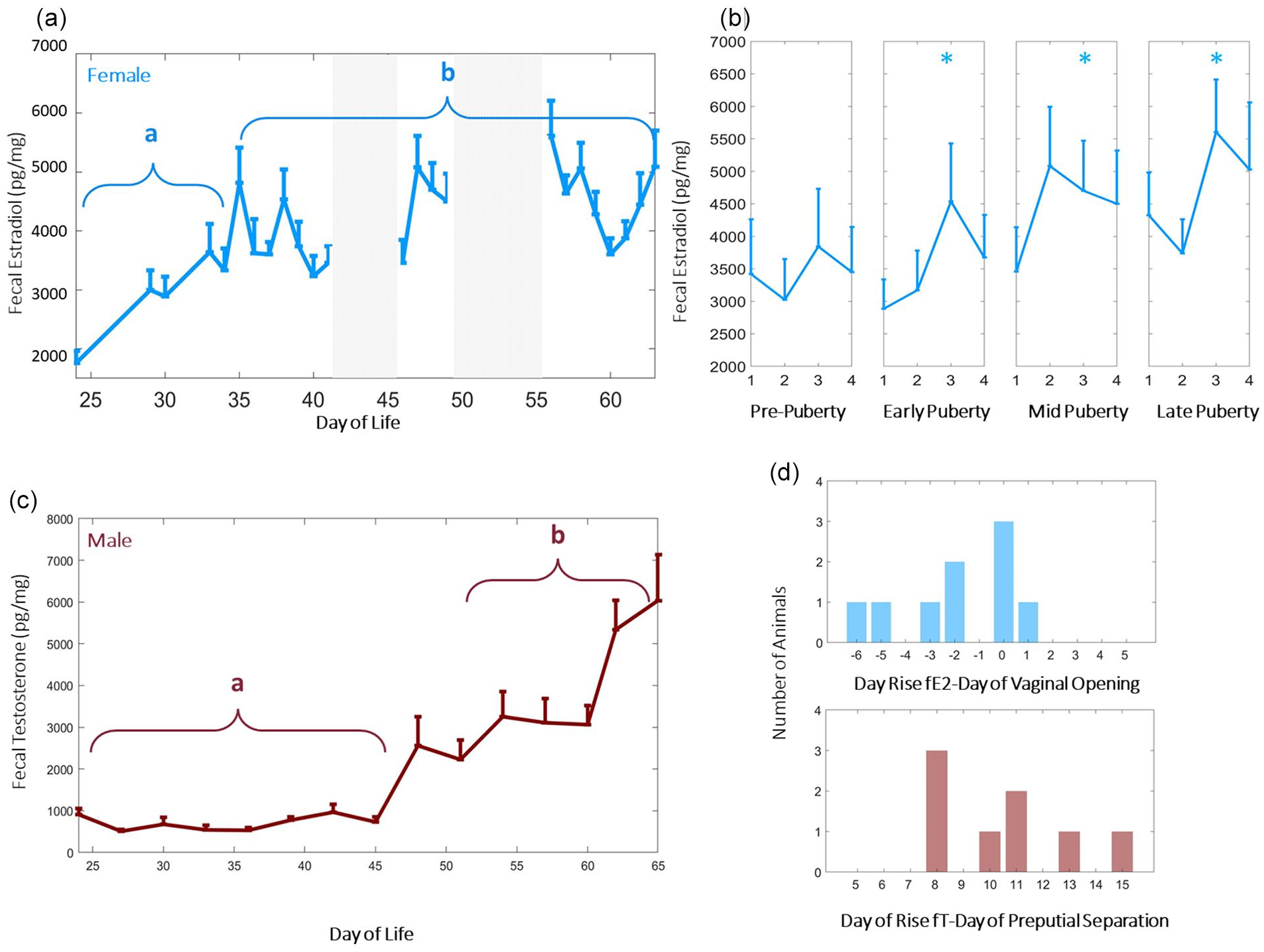
High frequency measurement of fecal estradiol and testosterone enables monitoring of estrous cycle emergence and pubertal progression in semi-naturalistic conditions. Group mean (±SEM) of female fecal estradiol (blue, a) and male (red, c) fecal testosterone. Fecal testosterone (fT) by day of life differed significantly after p45 (c), whereas the commencement of the ovulatory cycle contributed to variability of female fecal estradiol (a, b). *Letters signify Kruskal-Wallis group differences of fT values over the bracketed time region. Group mean and SEM of female (light blue, b). Fecal estradiol adopted a 4-day cycle that stabilized from early to late puberty, with levels elevated significantly (p = 0.001) by late adolescence. *Indicates significantly elevated fE2 levels in cycle as compared with pre-pubertal state. Fecal estradiol rose 2 standard deviations prior to vaginal opening in most females (d, top), but fecal testosterone rose 2 standard deviations ~1 to 2 weeks after preputial separation in males (d, bottom). Gray-shaded regions of the figure are time points at which fecal samples were not collected. Color version of the figure is available online.

Results

High-Frequency Fecal Estradiol and Testosterone Measurement Enable Monitoring of Pubertal Progression Under Semi-naturalistic Conditions

In females, fecal estradiol (fE2) increased after p35 (χ² = 9.80, p = 0.001), and exhibited periodic days of elevated fE2 thereafter (p = 0.03 for days 3 vs. day 1 after pubertal onset; Figure 1a and 1b). In males, fecal testosterone (fT) increased after p45 (χ² = 9.60, p = 0.002; Figure 1b). The relationship between canonical external signs of pubertal onset and fE2/fT rise was dependent on sex: fE2 rose 2 standard deviations prior to vaginal opening in most females (Figure 1d, top), whereas fT rose 2 standard deviations 1 to 2 weeks after preputial separation in males (Figure 1d, bottom). Weight trajectories for males and females were typical (Supplemental Figure 2).

Sex Differences in Circadian Power Are Present From Pre-adolescence Through Adulthood

CR but not UR power rose across early adolescence in both sexes (CR power upward trend: p = 0.009 and 0.0012 for females and males, respectively; UR power: p = 0.148 and 0.243 for both females and males, respectively; Figure 2a-2c). Males maintained statistically significantly higher CR power from pre-adolescence to mid-adolescence and in early adulthood (χ² = 8.00, 3.78, 16.53; p = 0.005, 0.052, 4.79 × 10^–5 for pre- to mid-adolescence, mid- to late adolescence, and late adolescence to early adulthood, respectively; Figure 2d-2f). CR power was positively correlated with fE2 in adolescent females (p = 0.04, r² = 0.08, Akaike information criterion [AIC] = −264; Figure 2g), whereas adolescent males did not exhibit a significant correlation between CR power and fE2 (p = 0.07, r² = 0.09, AIC = −132; Figure 2h). This pattern was not present prior to pubertal onset, defined by vaginal opening or preputial separation, in either sex (p = 0.54 and 0.89 for females and males, respectively; Figure 2g and 2h, insets).

Figure 2.

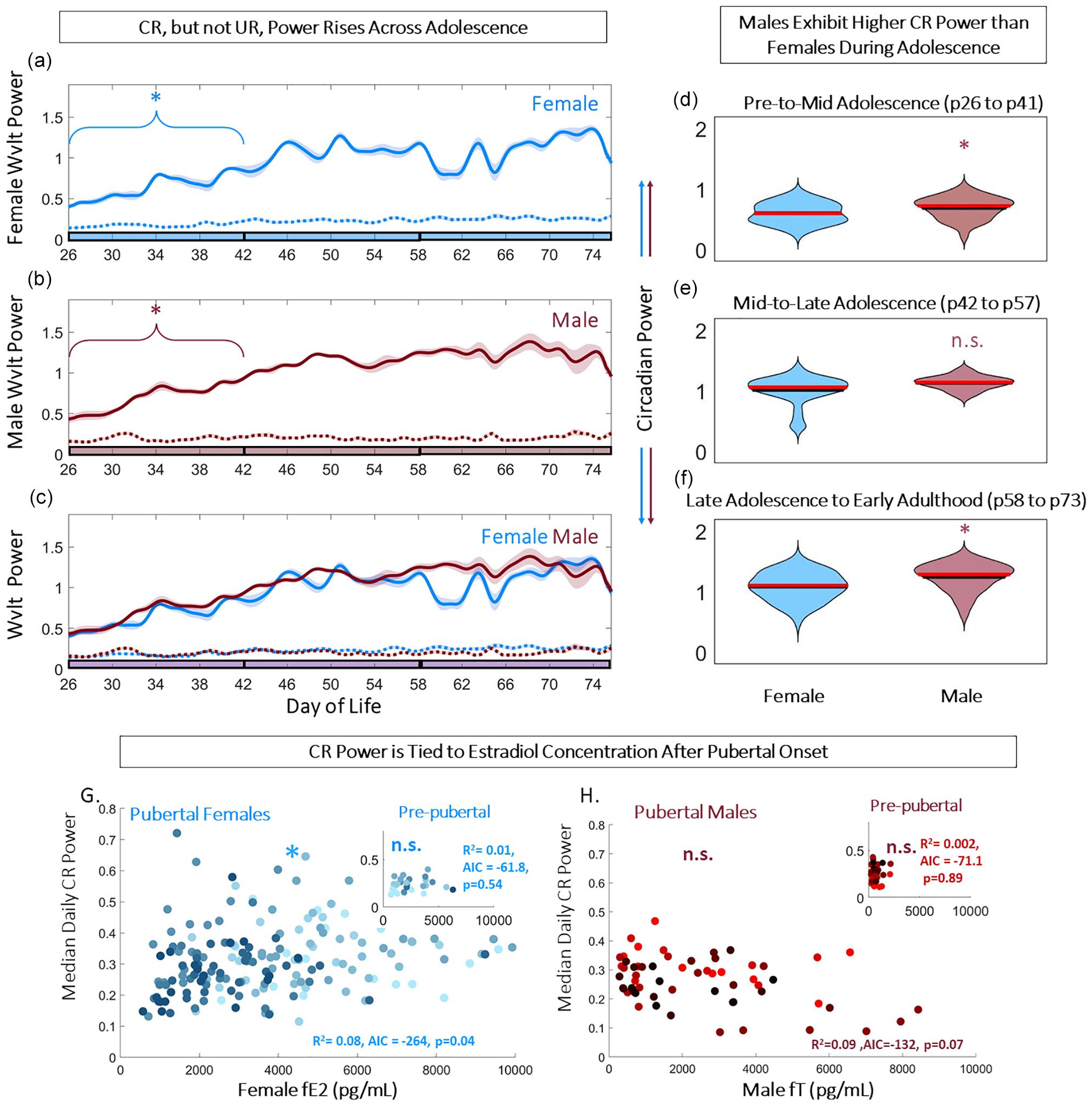
Adolescence exaggerates sex differences in circadian power and their correlation with sex steroids. Circadian but not ultradian power rises across early adolescence in both sexes (a-c). Linear plots of group mean (±SEM) of CBT circadian (solid) and ultradian (dashed) power in females (blue, a) and males (red, b), overlaid in (c). *Indicates significant trend over time for the bracketed time (p = 0.009 and 0.0012 for females and males, respectively). Phase of adolescence cutoffs (early to mid, mid to late, and late to adult) are indicated by breaks in the colored x-axis at p42 and p58. Violin plots of circadian power illustrate that males maintain significantly (letter indicates group difference) higher circadian power than females from early in life (d-f) (χ² = 8.00, 3.78, 16.53; p = 0.005, 0.052, 4.79 × 10^–5 for pre- to mid-adolescence, mid- to late adolescence, and late adolescence to early adulthood, respectively). Scatterplots of fE2 (g) and fT (h) by median daily circadian power in females and males, respectively, illustrate a female-specific positive correlation (p = 0.04, r² = 0.08, AIC = −264). This correlation is not present prior to pubertal onset (g, h, insets). Abbreviations: AIC = Akaike information criterion; CBT = core body temperature; CR = circadian rhythm; UR = ultradian rhythm. Color version of the figure is available online.

CBT and Ultradian Power Exhibite Sex-Specific Changes

CBT exhibited an approximately 4-day periodic fluctuation in females, but not males, commencing with the rise in fE2 and vaginal opening (χ² = 11.5, 1.3, p = 0.005 and 0.198 for females and males, respectively; Figure 3a and 3b). UR power exhibited a comparable 4-day pattern in females (χ² = 8.75, p = 0.034) but not males (χ² = 3.25, p = 0.169) (Figure 3a and 3b). A Fast Fourier Transform (FFT) of male and female CBT and UR power corroborated these observations; females exhibited statistically greater AUC for 4- to 5-day periodicity of CBT modulation (χ² = 11.29, p = 8 × 10^–4 for sex difference in AUC of 4- to 5-day temperature FFT; Figure 3c) and UR modulation (χ² = 9.28, p = 0.002 for sex difference in AUC of 4- to 5-day UR Power FFT; UR alignment shown in Figure 3d). In addition, females exhibited a statistically significant upward trend in temperature from pre- to mid-adolescence (p = 1 × 10^–5 to p = 0.02; mean p = 0.004), and a significant downward trend in body temperature from mid- to late adolescence (p = 0.019) (Figure 4a and 4c). Conversely, males did not exhibit a statistical trend in temperature from early to mid (p = 0.07) or from mid to late adolescence (p = 0.12) (Figure 4b and 4c). Violin plots of temperatures across adolescence indicated that females exhibited elevated temperatures compared with males for the entire period of study (χ² = 25.37, 33.84, 25.52; p = 9.75 × 10^–7, 5.97 × 10^–9, 4.37 × 10^–7 for pre- to mid-adolescence, mid- to late adolescence, and late adolescence to early adulthood, respectively; Figures 3a and 3b, 4d, and 4f).

Figure 3.

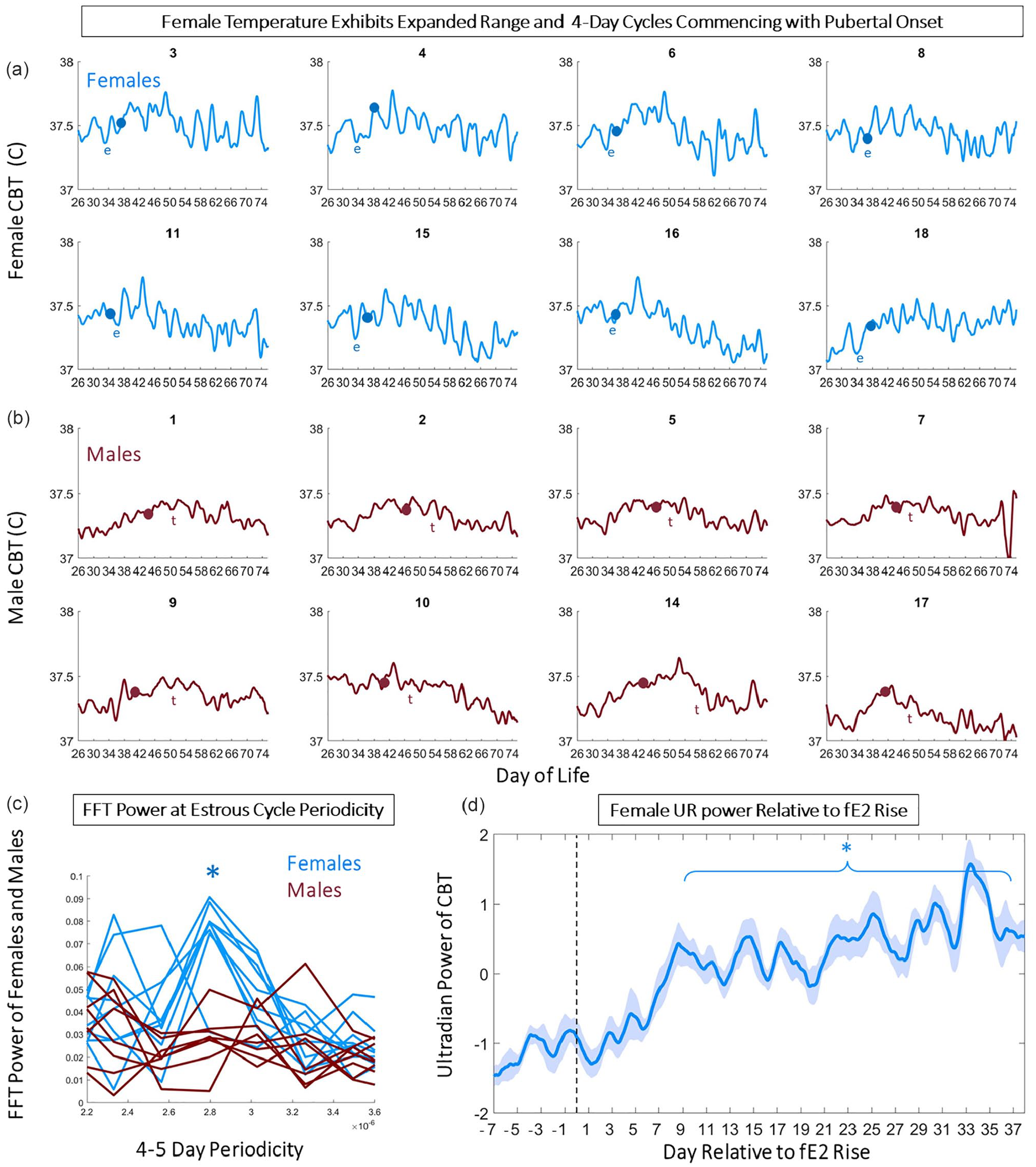
Four-day patterns of temperature and ultradian power track ovulatory cycles of after pubertal onset. Linear plots of smoothed temperature illustrate estrous cycles which onset in time with markers of puberty, vaginal opening, and rise in fecal estradiol in all individual females (a), and preputial separation and rise in fecal testosterone in males (b). Dots indicate day of vaginal opening (blue) or preputial separation (red). Letter “e” indicates day of first rise in fE2 >2 standard deviations above the mean, whereas letter “t” indicates day of first rise in fT >2 standard deviations above the mean. FFT of temperatures of females and males centered on 4- to 5-day periodicities indicate females (blue) exhibited a significant peak compared with males (red) (c, p = 8 × 10^–4). Mean (±SEM) of CBT ultradian power aligned among individuals with reference to first fE2 exhibits onset of 4- to 5-day modulation among females approximately 1 week after fE2 rise (d). Abbreviations: CBT = core body temperature; FFT = Fast Fourier Transform; UR = ultradian rhythm. Color version of the figure is available online.

Figure 4.

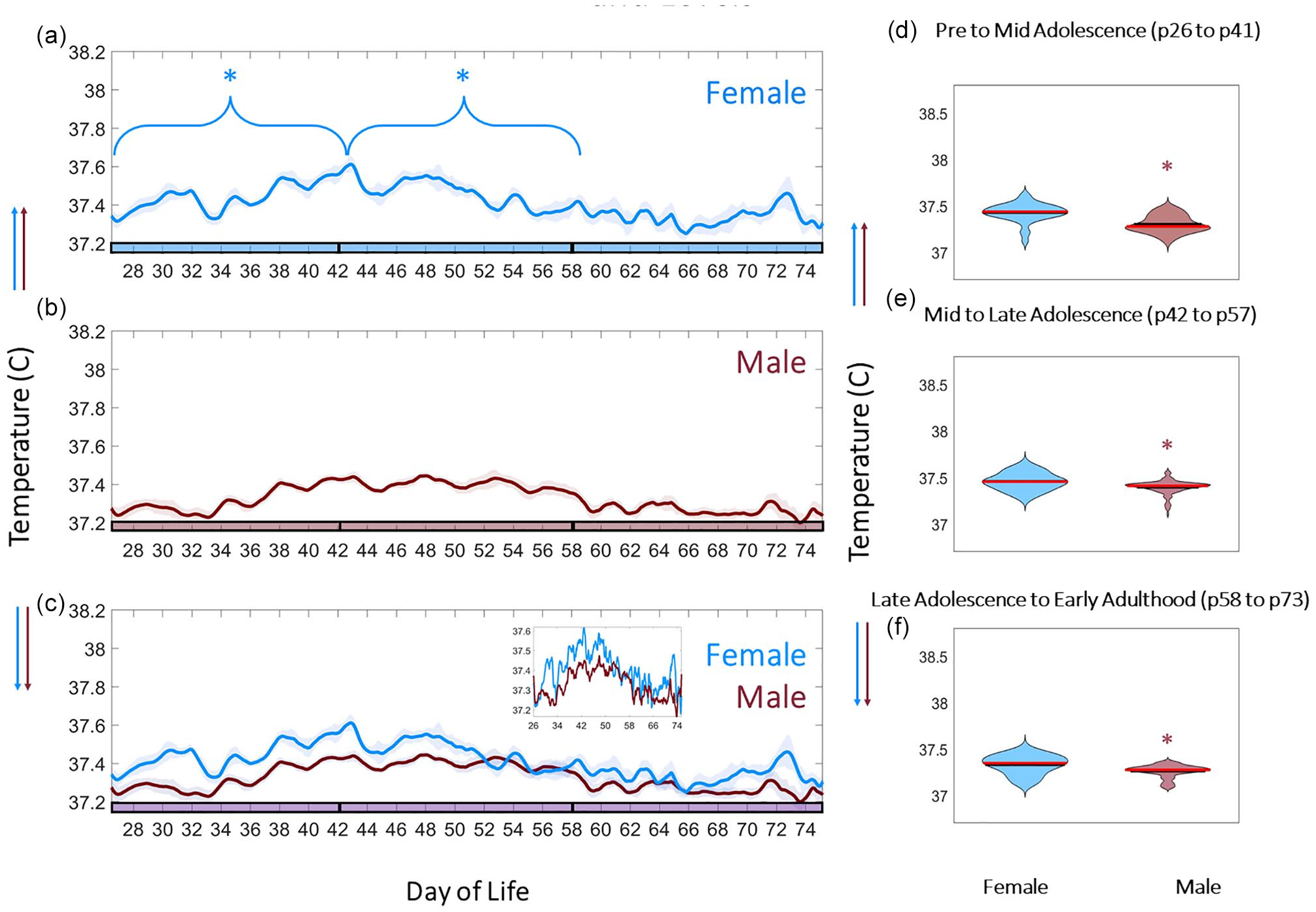
Adolescence is associated with sex-dependent CBT trends and levels. CBT linear group means (±SEM) in females (blue, a) and males (red, b). *Indicates statistically significant MK trend during the bracketed time period. Phase of adolescence cutoffs (pre to mid, mid to late, and late to adult) are indicated by breaks in the colored x-axis at p42 and p58. Females exhibit a statistically significant upward trend in body temperature from pre- to mid-adolescence (a-c) (p = 0.004), and a downward trend in body temperature from mid- to late adolescence (a) (p = 0.019). Violin plots of female and male temperatures across adolescence indicate that females exhibit wider ranging (* in d-f indicates significant difference) and elevated temperatures compared with males (c, zoomed inset; d-f) (χ² = 25.37, 33.84, 25.52; p = 9.75 × 10^–7, 5.97 × 10^–9, 4.37 × 10^–7 for pre- to mid-adolescence, mid- to late adolescence, and late adolescence to early adulthood, respectively). Abbreviations: CBT = core body temperature; MK = Mann Kendall. Color version of the figure is available online.

Discussion and Conclusion

The present findings reveal that CBT features measured in a semi-naturalistic environment can be used to monitor adolescent development, with features persisting in the presence of additional variability of sex steroid concentrations and environmental factors. Adolescent trends in CBT and CBT rhythmicity observed in the present study were akin to those of females and males examined in the laboratory (Grant et al., 2021; Kittrell and Satinoff, 1986) with notable sex differences. Males and females exhibited differential trends and amplitude in CR and UR power, with the most prominent being the rapid onset of ovulatory CBT rhythms in females following the early pubertal rise in fE2 and vaginal opening. CR power increased from pre- to mid-puberty in both sexes, with females exhibiting higher pubertal CBT and lower CR power than males. Despite the observation of higher and more variable fE2 compared with lab-reported values, females retained a statistically significant correlation between fE2 and CR power after pubertal onset (Grant et al., 2021). In contrast to the coordinated patterns in fE2 and CBT in females, coordinated changes in CBT structure and testosterone were not observed in males. Although the present study does not fully mimic conditions of the natural environment (e.g., foraging for food, burrows, broad interactions with conspecifics), the findings affirm that CBT and CBT rhythmicity remain informative in variable environments, particularly in females, and support the potential for using CBT outside of the laboratory environment and across species.

The similarity among the trajectories of circadian power in males and females is intriguing given that, consistent with previous findings, fT rose much later in males than did fE2 in females (Hagenauer et al., 2011; MacKinnon et al., 1978; Sengupta, 2013). Because the rise in fT was temporally decoupled from rhythmic metrics and preputial separation, a sex-steroid-independent change might drive development of male CBT rhythmicity. This finding was unexpected as androgen receptors are highly expressed in male suprachiasmatic core (Iwahana et al., 2008) and testosterone is necessary for the maintenance of typical circadian CBT and activity rhythms in adulthood (Butler et al., 2012; Karatsoreos et al., 2011; Morin and Cummings, 1981; Zuloaga et al., 2009). Numerous other hormonal and behavioral factors have been proposed to influence the timing of circadian consolidation of male activity and temperature, including melatonin (Cavallo, 1993; Rivest et al., 1986), growth hormone (Dunger et al., 1991; Grant et al., 2018), time since weaning (Joutsiniemi et al., 1991), and social interaction (Castro and Andrade, 2005). In addition, there are previous reports of increased time taken for circadian consolidation of activity in males (e.g., Cambras and Díez-Noguera, 1988; Díez-Noguera and Cambras, 1990) and of female-specific ties between estradiol and circadian period/consolidation (Alvord et al., 2021; Blattner and Mahoney, 2013; Morin et al., 1977; Takahashi and Menaker, 1980; Thomas and Armstrong, 1989; Wollnik and Döhler, 1986).

As indicated previously, males and females integrate numerous cues to trigger the onset of puberty and circadian consolidation, and estradiol contributes to coupling these processes in females (Weinert, 2005). The present results corroborate a female-specific relationship among body temperature, UR and CR development, and estradiol that exists at least from around the time of pubertal onset. Furthermore, despite some remarkable similarities in adolescent circadian, ultradian, and CBT trajectories between the sexes, the presence of elevated CBT (which persists into adulthood; Zuloaga et al., 2009) and reduced circadian power in females suggests that continuous-temperature-based diagnostic algorithms should take sex into account during training and validation. Although it would be fruitful to explore the phase relationship between sunrise/sunset across puberty under semi-natural conditions as performed in previous laboratory studies (Hagenauer et al., 2011), because individuals progress through puberty at different rates, day length is not the same across individuals at different stages of development in the present study. Larger cohorts, where puberty is synchronized among animals under naturalistic conditions, will help to uncover specific relationships among steroidal hormone trajectories, pubertal stage, and circadian phase under naturalistic conditions.

If the features described here have analogous counterparts in teen populations as suggested previously (e.g., Batinga et al., 2015; Pronina et al., 2015), and has recently been shown for continuous temperature for female luteinizing hormone surge anticipation (Grant et al., 2020; Webster and Smarr, 2020) and pregnancy (Grant et al., 2021), then this approach can be applied to develop powerful tools to further understand key developmental events. At present, children in developed nations begin puberty at an earlier age than in past decades, attributed to body fat and stress-related factors (Bellis et al., 2006, p. 12; Chittwar et al., 2012; Delemarre-van de Waal et al., 2002; Herbison, 2016; Parent et al., 2003). In addition, these children are subject to widely varying temporal disruptions in the form of light at night (Casper and Gladanac, 2014; Jain Gupta and Khare, 2020; Smarr and Schirmer, 2018), late meals (Jain Gupta and Khare, 2020), and female hormonal contraceptives (Apter, 2018). Despite the need for monitoring the effects and interactions of these variables on pubertal health, clinicians are equipped with relatively low temporal resolution tools for pubertal staging and diagnosis (Elchuri and Momen, 2020; Klein et al., 2017; Lauffer et al., 2020), and rhythmic stability throughout adolescent development is not considered by families or pediatricians (Owens and Weiss, 2017).

Together, non-invasive sex steroid measurement and chronic observation of CBT rhythms and amplitude represent promising metrics for the detection of pubertal onset and monitoring of the developmental trajectory in both sexes under semi-naturalistic conditions. Future work is needed to determine the extent to which such features are extant and coordinated with markers of puberty in humans, but the present findings in rats suggest the feasibility of such an approach.

Supplemental Material

sj-tiff-1-jbr-10.1177_07487304221092715 – Supplemental material for Sex Differences in Pubertal Circadian and Ultradian Rhythmic Development Under Semi-naturalistic Conditions

Supplemental material, sj-tiff-1-jbr-10.1177_07487304221092715 for Sex Differences in Pubertal Circadian and Ultradian Rhythmic Development Under Semi-naturalistic Conditions by Azure D. Grant, Linda Wilbrecht and Lance J. Kriegsfeld in Journal of Biological Rhythms

Supplemental Material

sj-tiff-2-jbr-10.1177_07487304221092715 – Supplemental material for Sex Differences in Pubertal Circadian and Ultradian Rhythmic Development Under Semi-naturalistic Conditions

Supplemental material, sj-tiff-2-jbr-10.1177_07487304221092715 for Sex Differences in Pubertal Circadian and Ultradian Rhythmic Development Under Semi-naturalistic Conditions by Azure D. Grant, Linda Wilbrecht and Lance J. Kriegsfeld in Journal of Biological Rhythms

Footnotes

Acknowledgements

The authors would like to thank Andrew Ahn, Ronald Dahl, Frédéric Theunissen, and Albert Qü for their helpful feedback on methods. This work was supported by a Miller Professorship from the Miller Institute for Basic Research at UC Berkeley (L.W.) and by National Institutes of Health Grant HD-050470 (L.J.K.).

Conflict of Interest Statement

The author(s) have no potential conflicts of interest with respect to the research, authorship, and/or publication of this article.

ORCID iD

Lance J. Kriegsfeld

Notes

References

Albertsson-Wikland

Rosberg

Lannering

Dunkel

Selstam

Norjavaara

(1997) Twenty-four-hour profiles of luteinizing hormone, follicle-stimulating hormone, testosterone, and estradiol levels: a semilongitudinal study throughout puberty in healthy boys. J Clin Endocrinol Metab 82:541-549.

Alvord

Kantra

Pendergast

(2021) Estrogens and the circadian system. Semin Cel Dev Biol S1084-9521(21)00083-5.

Ankarberg

Norjavaara

(1999) Diurnal rhythm of testosterone secretion before and throughout puberty in healthy girls: correlation with 17beta-estradiol and dehydroepiandrosterone sulfate. J Clin Endocrinol Metab 84:975-984.

Apter

(2018) Contraception options: aspects unique to adolescent and young adult. Best Pract Res Clin Obstet Gynaecol 48:115-127.

Asimes

Kim

Cuarenta

Auger

Pak

(2018) Binge drinking and intergenerational implications: parental preconception alcohol impacts offspring development in rats. J Endocr Soc 2:672-686.

Auer

Kußmaul

Möstl

Hohlbaum

Rülicke

Palme

(2020) Measurement of fecal testosterone metabolites in mice: replacement of invasive techniques. Animals 10:165.

Bakshi

Geyer

(1999) Ontogeny of isolation rearing-induced deficits in sensorimotor gating in rats. Physiol Behav 67:385-392.

Batinga

Martinez-Nicolas

Zornoza-Moreno

Sánchez-Solis

Larqué

Mondéjar

Moreno-Casbas

García

Campos

Rol

, et al. (2015) Ontogeny and aging of the distal skin temperature rhythm in humans. Age (Dordr) 37:29.

Bellis

Downing

Ashton

(2006) Adults at 12? Trends in puberty and their public health consequences. J Epidemiol Community Health 60:910-911.

10.

Bhavani

Carey

Gilbert

Afshar

Verhoef

Churpek

(2019) Identifying novel sepsis subphenotypes using temperature trajectories. Am J Respir Crit Care Med 200:327-335.

11.

Blattner

Mahoney

(2013) Photic phase-response curve in 2 strains of mice with impaired responsiveness to estrogens. J Biol Rhythms 28:291-300.

12.

Boggiano

Cavigelli

Dorsey

Kelley

CEP

Ragan

Chandler-Laney

(2008) Effect of a cage divider permitting social stimuli on stress and food intake in rats. Physiol Behav 95:222-228.

13.

Bourguignon

(1988) Time-related neuroendocrine manifestations of puberty: a combined clinical and experimental approach extracted from the 4th Belgian Endocrine Society lecture. Horm Res 30:224-234.

14.

Brown-Douglas

Firth

Parkinson

Fennessy

(2004) Onset of puberty in pasture-raised thoroughbreds born in southern hemisphere spring and autumn. Equine Vet J 36:499-504.

15.

Butler

Karatsoreos

LeSauter

Silver

(2012) Dose-dependent effects of androgens on the circadian timing system and its response to light. Endocrinology 153:2344-2352.

16.

Buxton

Atkinson

(1948) Hormonal factors involved in the regulation of basal body temperature during the menstrual cycle and pregnancy. J Clin Endocrinol Metab 8:544-549.

17.

Cambras

Díez-Noguera

(1988) Changes in motor activity during the development of the circadian rhythm in the rat. J Interdiscip Cycle Res 19:65-74.

18.

Casper

Gladanac

(2014) Introduction: circadian rhythm and its disruption: impact on reproductive function. Fertil Steril 102:319-320.

19.

Castro

ECV

Andrade

MMM

(2005) Longitudinal study of the spectral composition of behavioral rhythms in the rat. Biol Rhythm Res 36:131-140.

20.

Cavallo

(1993) Melatonin and human puberty: current perspectives. J Pineal Res 15:115-121.

21.

Chittwar

Shivprakash Ammini

(2012) Precocious puberty in girls. Indian J Endocrinol Metab 16:S188-S191.

22.

Daan

Slopsema

(1978) Short-term rhythms in foraging behaviour of the common vole, Microtus arvalis. J Comp Physiol 127:215-227.

23.

de Kloet

Sarabdjitsingh

(2008) Everything has rhythm: focus on glucocorticoid pulsatility. Endocrinology 149:3241-3243.

24.

Delemarre-van de Waal

van Coeverden

SCCM

Engelbregt

MTJ

(2002) Factors affecting onset of puberty. Horm Res 57:15-18.

25.

Díez-Noguera

Cambras

(1990) Sex differences in the development of the motor activity circadian rhythm in rats under constant light. Physiol Behav 47:889-894.

26.

Dunger

Matthews

Edge

Jones

Preece

(1991) Evidence for temporal coupling of growth hormone, prolactin, LH and FSH pulsatility overnight during normal puberty. J Endocrinol 130:141-149.

27.

Elchuri

Momen

(2020) Disorders of pubertal onset. Prim Care 47:189-216.

28.

Franklin

Waddell

Behrns

Goodrowe

(2020) Estrous cyclicity and reproductive success are unaffected by translocation for the formation of new reproductive pairs in captive red wolves (Canis rufus). Zoo Biol 39:230-238.

29.

Garcia

Rosen

Mahowald

(2001) Circadian rhythms and circadian rhythm disorders in children and adolescents. Semin Pediatr Neurol 8:229-240.

30.

Goh

Maloney

Mark

Blache

(2019) Episodic ultradian events—ultradian rhythms. Biology 8:15.

31.

Grant

Newman

Kriegsfeld

(2020) Ultradian rhythms in heart rate variability and distal body temperature anticipate onset of the luteinizing hormone surge. Sci Rep 10:20378.

32.

Grant

Wilbrecht

Kriegsfeld

(2021) Adolescent development of biological rhythms in female rats: estradiol dependence and effects of combined contraceptives. Front Physiol 12:752363.

33.

Grant

Wilsterman

Smarr

Kriegsfeld

(2018) Evidence for a coupled oscillator model of endocrine ultradian rhythms. J Biol Rhythms 33:475-496.

34.

Hagenauer

Lee

(2012) The neuroendocrine control of the circadian system: adolescent chronotype. Front Neuroendocrinol 33:211-229.

35.

Hagenauer

King

Possidente

McGinnis

Lumia

Peckham

Lee

(2011) Changes in circadian rhythms during puberty in Rattus norvegicus: developmental time course and gonadal dependency. Horm Behav 60:46-57.

36.

Harper

Austad

(2000) Fecal glucocorticoids: a noninvasive method of measuring adrenal activity in wild and captive rodents. Physiol Biochem Zool 73:12-22.

37.

Herbison

(2016) Control of puberty onset and fertility by gonadotropin-releasing hormone neurons. Nat Rev Endocrinol 12:452-466.

38.

Hoogenboom

Daan

Dallinga

Schoenmakers

(1984) Seasonal change in the daily timing of behaviour of the common vole, Microtus arvalis. Oecologia 61:18-31.

39.

Iwahana

Karatsoreos

Shibata

Silver

(2008) Gonadectomy reveals sex differences in circadian rhythms and suprachiasmatic nucleus androgen receptors in mice. Horm Behav 53:422-430.

40.

Jain Gupta

Khare

(2020) Disruption in daily eating-fasting and activity-rest cycles in Indian adolescents attending school. PLoS ONE 15:e0227002.

41.

Joutsiniemi

Leinonen

Laakso

(1991) Continuous recording of locomotor activity in groups of rats: postweaning maturation. Physiol Behav 50:649-654.

42.

Joyce

Zele

Feigl

Adhikari

(2020) The accuracy of artificial and natural light measurements by actigraphs. J Sleep Res 29:e12963.

43.

Kalliokoski

Teilmann

Abelson

KSP

Hau

(2015) The distorting effect of varying diets on fecal glucocorticoid measurements as indicators of stress: a cautionary demonstration using laboratory mice. Gen Comp Endocrinol 211:147-153.

44.

Karatsoreos

Butler

LeSauter

Silver

(2011) Androgens modulate structure and function of the suprachiasmatic nucleus brain clock. Endocrinology 152:1970-1978.

45.

Kim

Harrington

(2008) Neuropeptide Y-deficient mice show altered circadian response to simulated natural photoperiod. Brain Res 1246:96-100.

46.

Kittrell

EMW

Satinoff

(1986) Development of the circadian rhythm of body temperature in rats. Physiol Behav 38:99-104.

47.

Klein

Emerick

Sylvester

Vogt

(2017) Disorders of puberty: an approach to diagnosis and management. Am Fam Physician 96:590-599.

48.

Kottler

Coussieu

Valensi

Levi

Degrelle

(1989) Ultradian, circadian and seasonal variations of plasma progesterone and LH concentrations during the luteal phase. Chronobiol Int 6:267-277.

49.

Kriegsfeld-Lab (2021) GitHub [WWW document]. [accessed 2021 May 24]. https://github.com/Kriegsfeld-Lab.

50.

Lafaille

Gouat

Féron

(2015) Efficiency of delayed reproduction in Mus spicilegus. Reprod Fertil Dev 27:491-496.

51.

Lauffer

Mooij

Zwaveling-Soonawala

van Trotsenburg

ASP

(2020) Reforming the male Tanner genital scale. J Pediatr Endocrinol Metab 33:425-426.

52.

Leise

(2013) Wavelet analysis of circadian and ultradian behavioral rhythms. J Circadian Rhythms 11:5.

53.

Leise

(2015) Chapter five—wavelet-based analysis of circadian behavioral rhythms. In: Sehgal

, editor. Methods in enzymology. Part A: circadian rhythms and biological clocks. San Diego (CA): Academic Press. p. 95-119.

54.

Lewis

Curtis

(2016) Male prairie voles display cardiovascular dipping associated with an ultradian activity cycle. Physiol Behav 156:106-116.

55.

Lilly

Olhede

(2012) Generalized Morse wavelets as a superfamily of analytic wavelets. IEEE Trans Signal Process 60:6036-6041.

56.

Huang

Hua

Chen

Timm

Maclin

Haggerty

Aust

Golden

, et al. (2020) Reprogramming of ovarian granulosa cells by YAP1 leads to development of high-grade cancer with mesenchymal lineage and serous features. Sci Bull 65:1281-1296.

57.

MacKinnon

Puig-Duran

Laynes

(1978) Reflections on the attainment of puberty in the rat: have circadian signals a role to play in its onset? J Reprod Fertil 52:401-412.

58.

Mathew

Gaikwad

Gonzalez

Nugent

Smith

(2017) Evaluation of active hexose correlated compound (AHCC) in combination with anticancer hormones in orthotopic breast cancer models. Integr Cancer Ther 16:300-307.

59.

Meijer

Michel

Vanderleest

Rohling

(2010) Daily and seasonal adaptation of the circadian clock requires plasticity of the SCN neuronal network. Eur J Neurosci 32:2143-2151.

60.

Millspaugh

Washburn

(2003) Within-sample variation of fecal glucocorticoid measurements. Gen Comp Endocrinol 132:21-26.

61.

Mohawk

Green

Takahashi

(2012) Central and peripheral circadian clocks in mammals. Annu Rev Neurosci 35:445-462.

62.

Morin

Cummings

(1981) Effect of surgical or photoperiodic castration, testosterone replacement or pinealectomy on male hamster running rhythmicity. Physiol Behav 26:825-838.

63.

Morin

Fitzgerald

Zucker

(1977) Estradiol shortens the period of hamster circadian rhythms. Science 196:305-307.

64.

Norjavaara

Ankarberg

Albertsson-Wikland

(1996) Diurnal rhythm of 17 beta-estradiol secretion throughout pubertal development in healthy girls: evaluation by a sensitive radioimmunoassay. J Clin Endocrinol Metab 81:4095-4102.

65.

Owens

Weiss

(2017) Insufficient sleep in adolescents: causes and consequences. Minerva Pediatr 69:326-336.

66.

Parent

Teilmann

Juul

Skakkebaek

Toppari

Bourguignon

(2003) The timing of normal puberty and the age limits of sexual precocity: variations around the world, secular trends, and changes after migration. Endocr Rev 24:668-693.

67.

Park

Spencer

Place

Jordan

Zucker

(2003) Seasonal control of penile development of Siberian hamsters (Phodopus sungorus) by daylength and testicular hormones. Reproduction 125:397-407.

68.

Pronina

Orlova

Rybakov

(2015) Circadian rhythm of skin temperature of children during puberty. Fiziol Cheloveka 41:74-84.

69.

Righetti

Tybur

Van Lange

Echelmeyer

van Esveld

Kroese

van Brecht

Gangestad

(2020) How reproductive hormonal changes affect relationship dynamics for women and men: a 15-day diary study. Biol Psychol 149:107784.

70.

Rivest

Aubert

Lang

Sizonenko

(1986) Puberty in the rat: modulation by melatonin and light. J Neural Transm 21:81-108.

71.

Sanchez-Alavez

Tabarean

Osborn

Mitsukawa

Schaefer

Dubins

Holmberg

Klein

Klaus

Gomez

, et al. (2010) Insulin causes hyperthermia by direct inhibition of warm-sensitive neurons. Diabetes 59:43-50.

72.

Sengupta

(2013) The laboratory rat: relating its age with human’s. Int J Prev Med 4:624-630.

73.

Silva

Domínguez

(2020) Clock control of mammalian reproductive cycles: looking beyond the pre-ovulatory surge of gonadotropins. Rev Endocr Metab Disord 21:149-163.

74.

Smarr

Schirmer

(2018) 4 million real-world learning management system logins reveal the majority of students experience social jet lag correlated with decreased performance. Sci Rep 8:4793.

75.

Smarr

Aschbacher

Fisher

Chowdhary

Dilchert

Puldon

Rao

Hecht

Mason

(2020) Feasibility of continuous fever monitoring using wearable devices. Sci Rep 10:21640.

76.

Smarr

Grant

Zucker

Prendergast

Kriegsfeld

(2017) Sex differences in variability across timescales in BALB/c mice. Biol Sex Differ 8:7.

77.

Smarr

Zucker

Kriegsfeld

(2016) Detection of successful and unsuccessful pregnancies in mice within hours of pairing through frequency analysis of high temporal resolution core body temperature data. PLoS ONE 11:e0160127.

78.

Steadman

(2019) The effect of spinal cord injury on sexual function. Louisville (KY): University of Louisville.

79.

Steadman

Hoey

Montgomery

Hubscher

(2019) Activity-based training alters penile reflex responses in a rat model of spinal cord injury. J Sex Med 16:1143-1154.

80.

Steiger

Valcu

Spoelstra

Helm

Wikelski

Kempenaers

(2013) When the sun never sets: diverse activity rhythms under continuous daylight in free-living arctic-breeding birds. Proc Biol Sci 280:20131016.

81.

Stothard

McHill

Depner

Birks

Moehlman

Ritchie

Guzzetti

Chinoy

LeBourgeois

Axelsson

, et al. (2017) Circadian entrainment to the natural light-dark cycle across seasons and the weekend. Curr Biol 27:508-513.

82.

Takahashi

Menaker

(1980) Interaction of estradiol and progesterone: effects on circadian locomotor rhythm of female golden hamsters. Am J Physiol 239:R497-504.

83.

Thomas

Armstrong

(1989) Effect of ovariectomy and estradiol on unity of female rat circadian rhythms. Am J Physiol 257:R1241-R1250.

84.

Touma

Palme

Sachser

(2004) Analyzing corticosterone metabolites in fecal samples of mice: a noninvasive technique to monitor stress hormones. Horm Behav 45:10-22.

85.

Vidal

(2017) The impact of age on the female reproductive system. Toxicol Pathol 45:206-215.

86.

Violin plots 101: visualizing distribution and probability density (2021) [WWW document]. [accessed 2021 Mar 3]. https://mode.com/blog/violin-plot-examples/.

87.

Webster

Smarr

(2020) Using circadian rhythm patterns of continuous core body temperature to improve fertility and pregnancy planning. J Circadian Rhythms 18:5.

88.

Weinert

(2005) Ontogenetic development of the mammalian circadian system. Chronobiol Int 22:179-205.

89.

Williams

Dacks

Rance

(2010) An improved method for recording tail skin temperature in the rat reveals changes during the estrous cycle and effects of ovarian steroids. Endocrinology 151:5389-5394.

90.

Wollnik

Döhler

(1986) Effects of adult or perinatal hormonal environment on ultradian rhythms in locomotor activity of laboratory LEW/Ztm rats. Physiol Behav 38:229-240.

91.

Woodruff

Lacey

Bentley

(2010) Contrasting fecal corticosterone metabolite levels in captive and free-living colonial tuco-tucos (Ctenomys sociabilis). J Exp Zool Part Ecol Genet Physiol 313A:498-507.

92.

Woodruff

Lacey

Bentley

Kriegsfeld

(2013) Effects of social environment on baseline glucocorticoid levels in a communally breeding rodent, the colonial tuco-tuco (Ctenomys sociabilis). Horm Behav 64:566-572.

93.

Zuloaga

McGivern

Handa

(2009) Organizational influence of the postnatal testosterone surge on the circadian rhythm of core body temperature of adult male rats. Brain Res 1268:68-75.

Supplementary Material

Please find the following supplemental material available below.

For Open Access articles published under a Creative Commons License, all supplemental material carries the same license as the article it is associated with.

For non-Open Access articles published, all supplemental material carries a non-exclusive license, and permission requests for re-use of supplemental material or any part of supplemental material shall be sent directly to the copyright owner as specified in the copyright notice associated with the article.

0.00 MB

0.23 MB

0.40 MB