
Abstract
Mathematical models have been used extensively in chronobiology to explore characteristics of biological clocks. In particular, for human circadian studies, the Kronauer model has been modified multiple times to describe rhythm production and responses to sensory input. This phenomenological model comprises a single set of parameters which can simulate circadian responses in humans under a variety of environmental conditions. However, corresponding models for nocturnal rodents commonly used in circadian rhythm studies are not available and may require new parameter values for different species and even strains. Moreover, due to a considerable variation in experimental data collected from mice of the same strain, within and across laboratories, a range of valid parameters is essential. This study develops a Kronauer-like model for mice by re-fitting relevant parameters to published phase response curve and period data using total least squares. Local parameter sensitivity analysis and parameter distributions determine the parameter ranges that give a near-identical model and data distribution of periods. However, the model required further parameter adjustments to match characteristics of other mouse strains, implying that the model itself detects changes in the core processes of rhythm generation and control. The model is a useful tool to understand and interpret future mouse circadian clock experiments.
The suprachiasmatic nucleus (SCN) is the site of the central clock in mammals and is responsible for regulating the body’s circadian cycles and influencing the response to various stimuli. Many important rhythms such as the sleep–wake cycle and body temperature cycle are circadian, and are thus controlled by the SCN. It has long been of great interest within the field of circadian biology to construct a working model of the SCN. However, due to the inherent coupled complexity of biological systems, determining the connections between genes, protein networks, neurons, and neuronal circuits and their relation to behavior has been a formidable task in both theoretical and experimental biology.
A phenomenological model of the human circadian pacemaker, originally by Kronauer (1990), has been developed, studied, and iterated upon over the last few decades (Phillips et al., 2011; St Hilaire et al., 2007a; Forger et al., 1999; Jewett et al., 1999; Kronauer et al., 1999; Klerman et al., 1996). Additional phenomena such as non-photic stimuli (St Hilaire et al., 2007a, 2007b) have been incorporated, while modifications to the model and changes to the parameter values have improved its accuracy in producing human phase response curve (PRC) and resetting data.
Other examples of general phenomenological models for mammals have been developed to understand the dynamics of the circadian clock, such as those by Daan and Berde (1978), Kawato and Suzuki (1980), and Schmal et al. (2020). However, to our knowledge, there does not exist a correspondence to the model by Kronauer (1990) that describes the circadian behavior in mice.
There are many mechanistic models that are used to decipher the molecular interactions underlying the circadian clock. These include the models of Herzel (Becker-Weimann et al., 2004a, 2004b), Forger (Forger and Peskin, 2003; Kim and Forger, 2012; Dewoskin et al., 2014), and others (Podkolodnaya et al., 2017; Mirsky et al., 2009; Lema et al., 2000). In addition, there are single-cell models of Relógio et al. (2011) and Shiju and Sriram (2017), and the multi-cell models of Vasalou and Henson (2010), To et al. (2007), and DeWoskin et al. (2015). However, these models are computationally expensive and difficult to corroborate with behavior. A simpler, phenomenological model is much more convenient for analysis and comparison with the available mice behavioral data for photic and non-photic inputs.
Given the similarities of the structure of the circadian clock between mice and humans, we reason that using the Van der Pol oscillator equations of the Kronauer model, originally developed for the human pacemaker, should also be suitable to model the mouse pacemaker. However, the parameter values used in the human model are not applicable to mice and do not result in good agreement with mouse experimental data. Furthermore, because the original human pacemaker parameters were fit based on an optimization approach that minimized the perpendicular distance to the data, these parameters are only suitable when describing the average process and fail to describe specific samples in the population.
Many authors have measured the free-running period of the wild-type C57BL/6 mouse in constant conditions and have reported widely varying results. It has been discussed in several of these studies that physical characteristics, such as age, may play an important role. In particular, it has been noted that the free-running period of the C57BL/6J mouse for wheel-running activity under constant dark conditions appears to lengthen with age (Mayeda et al., 1997; Possidente et al., 1995; Valentinuzzi et al., 1997). Other important factors that have been considered are the effects of access versus restriction to a running wheel (Capri et al., 2019); different types of white light (Alves-Simoes et al., 2016); particular wavelengths of light (Hofstetter et al., 2005); sub-strains of C57BL/6 mice, particularly that of the 6J and 6N varieties (Capri et al., 2019; Ebihara et al., 1978); and perhaps even the presence of light-induced retinal damage (Gonzalez, 2018).
In this article, we develop a fully functional phenomenological model of the mouse circadian clock. We focus on one of the most commonly used mouse strains: the wild-type C57BL/6 mouse. We use the existing formulation of the model (Kronauer, 1990), but re-fit the parameters to experimental PRC data. We demonstrate the robustness of the fit mouse parameters by validating against other PRCs available in the literature and comparing the results with that of the human model. Then, because of the large variation in the free-running period within and across labs, we perform a local sensitivity analysis to determine the most relevant parameters that affect the simulated period in constant conditions. With these relevant parameters, we deduce the range of potential values by parameter variation and fitting the simulated free-running period to the experimentally observed free-running periods in the literature. Finally, we demonstrate some applications of the mouse model: The model is used to deduce the maximal phase response to photic stimuli and the model is adapted to describe a mutant mouse.
Methods
Mathematical Model
To model the circadian pacemaker for mice, we begin with Kronauer’s oscillator model (Kronauer, 1990), derived from the Van der Pol oscillator, the proto-typical limit-cycle oscillator. The equations describing the evolution of the state of the circadian pacemaker, known as Process P, are as follows:
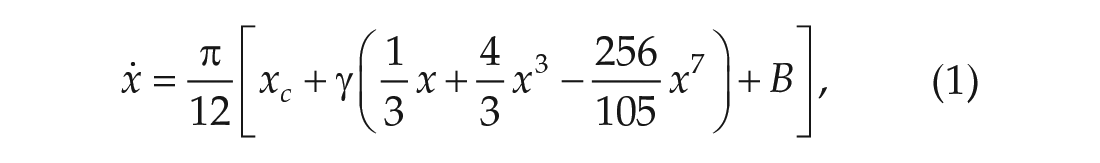
In the absence of light
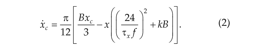
Process P is driven by light, through Process L, according to the following equations:


The variable
The parameter
MATLAB code for simulating the model and generating a PRC is available on ModelDB (McDougal et al., 2017) at http://modeldb.yale.edu/267250.
Fitting Data Sources
The model parameters were determined by fitting to data sets from Pendergast et al. (2010) and Vajtay et al. (2017) simultaneously. The experimental protocols for these data sets are described below.
Pendergast et al. (2010) set up singly housed wild-type C57BL/6J mice in a cage where they free-ran for 6 days in DD. The authors used linear regression to determine the onset of activity at 12 h circadian time (CT 12) on the following day and, at the appropriately calculated CT, the cages were transferred to another light-tight box and given light of 150 lx (measured at the cage bottom), where the mice ran for 15 min. Then, the mice were returned to DD and free-ran for a week.
Vajtay et al. (2017) entrained wild-type C57BL/6J mice (7-8 males) for 2 weeks under LD12:12 and then released them into DD. Every 14 days, the lights were turned on for 3 h at appropriate CTs. In this experiment, the authors note that the light was turned on such that the midpoint of the light exposure correlated with the appropriate CT of the mouse. The light intensities were in the range of 250 to 400 lx at bedding level. Each mouse had a total of 8 randomly timed light exposures. The phase shifts were then averaged for each 3-h bin, giving 5 to 9 measurements for each data point.
Validation Data Sources
For model validation, we did not alter our fit parameters and, following the respective light protocols and experimental setups, compared the simulation results against data from Vitaterna et al. (2006) and Comas et al. (2006).
Vitaterna et al. (2006) entrained C57BL/6J mice to a LD12:12 cycle for 1 week and subsequently released them into DD. After 3 weeks of free-running in DD, a 6-h light pulse was given at an appropriate CT, calculated from the period and onset of activity (CT 12). The data were collected for an additional 10 days in DD after the light pulse.
In Comas et al.’s (2006) experiments, C57BL/6J and C57BL/6J-OlaHsd mice were entrained for 2 weeks in LD12:12 so that the initial phases were all the same. The mice were then released into DD and given a pulse of light of 100 lx every 11 days.
As a further validation of the model parameters, and to demonstrate the sensitivity of the parameters to specific strains of mice, we also compared our model with the data for a non-C57BL/6J mouse. Ouk et al. (2019) used mice from a CBA × C57BL/6J background. The mice were entrained to an LD12:12 cycle for 7 to 10 days, followed by 10 to 14 days in DD. Then, at appropriate CTs, the mice were exposed to 15 min of white light at 300 lx. The data were collected for at least 10 to 14 days after the pulse to determine the phase shift calculations.
Fitting Procedure
The model fitting was performed in MATLAB using global parallel optimization, with the method of total least squares. The simulation was set up as follows. First, the “animal” is entrained to a 400 lx LD12:12 cycle, using an arbitrary initial condition on
The experiments did not report any error in the independent (time) variable; however, there is inherent uncertainty in determining the precise CTs for the light stimulus, which are calculated through linear regression. For this reason, it is more sensible to fit data according to the perpendicular distance between the data and the model curve. Thus, our objective function is defined to be the squared sum of the minimum Euclidean distance between each data point,

in which
Parameters
We modified parameter
Results
For our nominal parameters, it was determined that for
The optimal parameters determined by the fit are provided in Table 1.
A comparison of model parameters between the human model (St Hilaire et al., 2007b) and our mouse model.
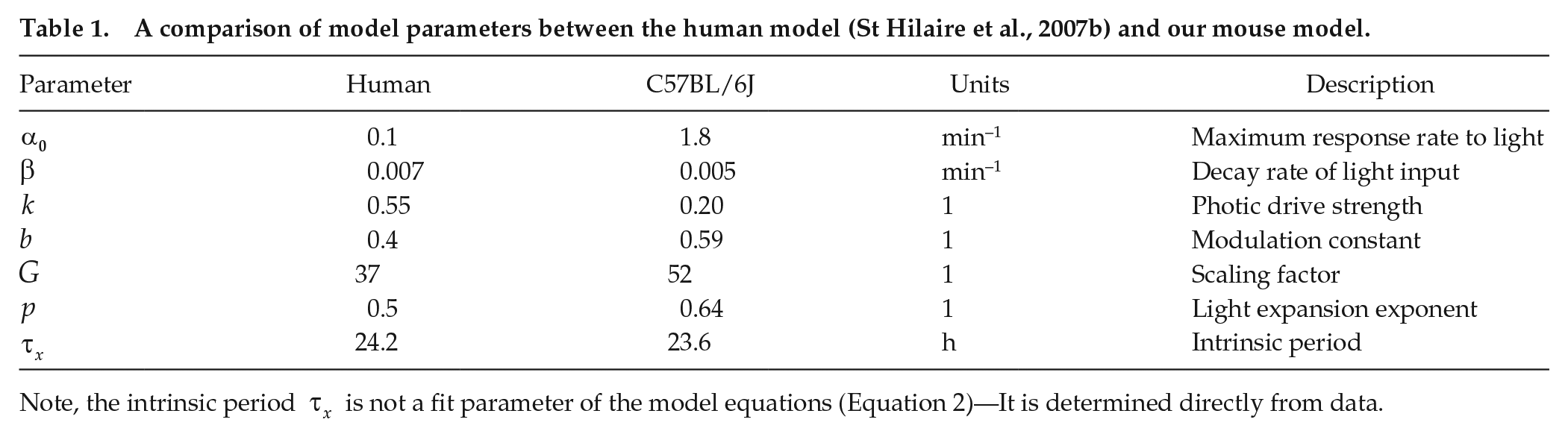
Note, the intrinsic period
The model parameters were fit against data from Pendergast et al. (2010) and Vajtay et al. (2017). The comparison between the optimal fit parameters and the experimental data is shown in Figure 1.
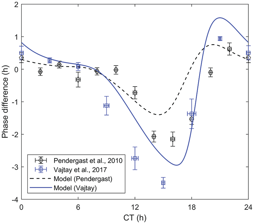
Fit model and experimental data as provided in Pendergast et al. (2010) and Vajtay et al. (2017). The phase difference was calculated as the average of the difference between the minimum of
The model was validated against data from Vitaterna et al. (2006) with the mouse model parameters (Table 1) providing a very good match with the experiment, as shown in Figure 2. The experimental data involved measuring the phase shift in 61 wild-type mice in response to 6-h light pulses at appropriate CTs. For a summary of the experimental protocols, see “Validation Data Sources” section. Data from a representative PRC for a 6-h light pulse in Nakamura et al. (2016) are included as well for comprehensiveness. In Figure 2, we also plot and compare our model PRC with the PRC generated using the human model parameters (Table 1). To be consistent, we have used identical prior photoperiods, LD12:12, for both the mouse and human simulations. One can clearly see that these parameters do not yield an appreciable phase response for the identical experimental protocol: The human model results in a maximum phase delay of 1.76 h and a maximum advance of 1.45 h, significantly lacking in both the advance and delay zones present in the data.
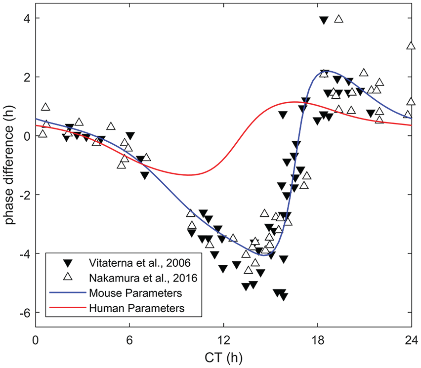
Validation against data for a light pulse of 6 h (Vitaterna et al., 2006; Nakamura et al., 2016) using the optimal mouse model parameters, compared with the human model parameters (Table 1). As in Figure 1, the phase difference was calculated as the average of the difference of minima before and after the light pulse. See Table 1 for parameter values. Abbreviation: CT = circadian time.
We have also compared our model simulations with that of Comas et al. (2006) for light pulses of duration 1, 3, 4, 6, 9, and 12 h, shown in Figure 3. We emphasize that the parameters (Table 1) were completely unaltered. From the figures below, it is clear the model provides an excellent match with the data, capturing the slight advance region in the early CTs and transition into the dead zone for pulses of 1 to 6 h, as well as the lack of a dead zone in the 9- and 12-h pulses.
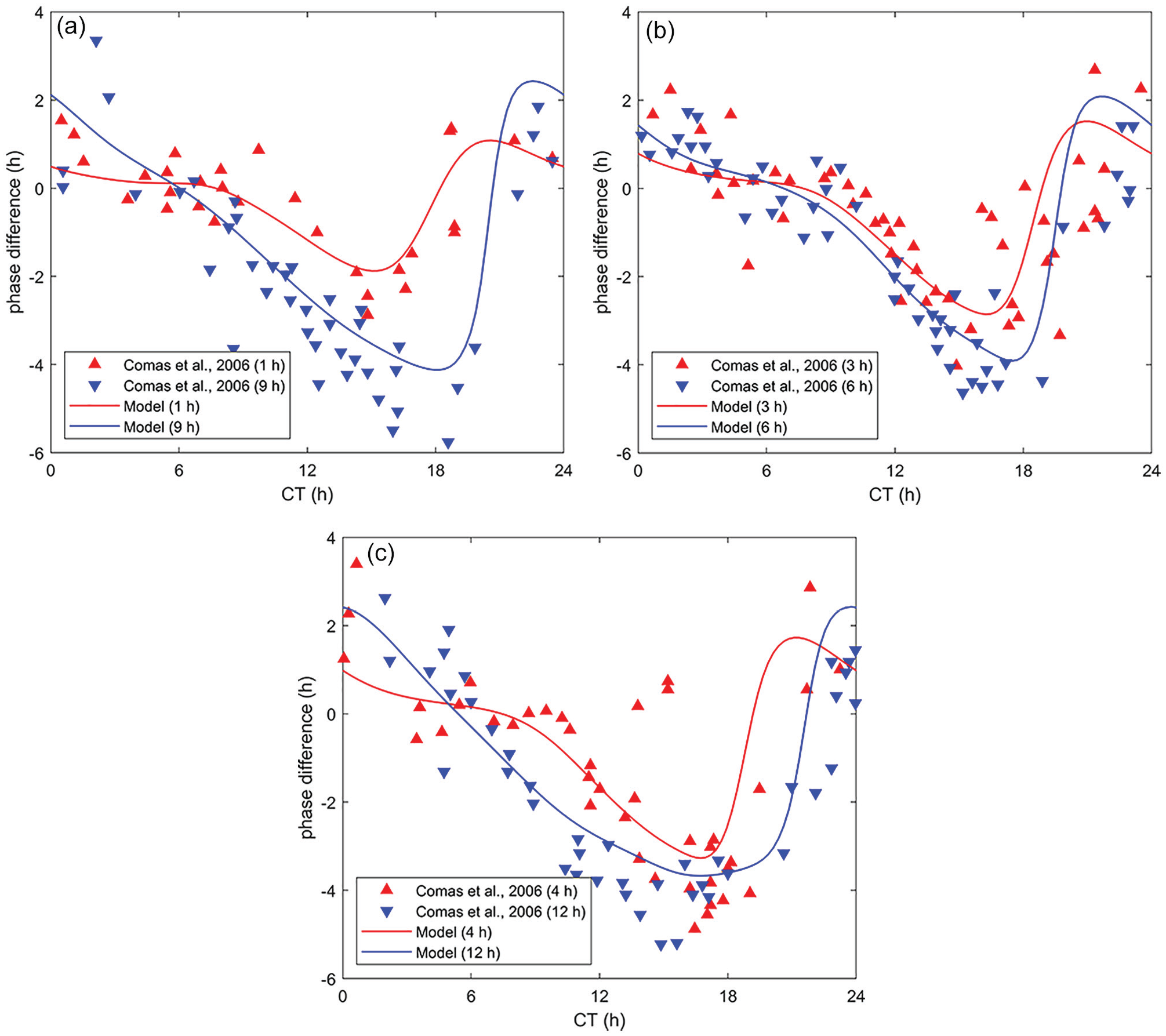
Validation with experimental data (Comas et al., 2006) for light pulses of duration (a) 1 h, 9 h; (b) 3 h, 6 h; and (c) 4 h, 12h at 100 lx. The mouse model demonstrates an excellent qualitative agreement with the data, clearly showing the lack of dead zones for the 9- and 12-h pulses as well as the gradual shift from slight advance to the dead zone to the delay zone in the other pulses. Abbreviation: CT = circadian time.
Figure 4 demonstrates another validation of the model. With the C57BL/6J mouse model parameters (Table 1), comparison of the generated model curves to the experimental data presented in Ouk et al. (2019) results in a poor match, particularly near the region of phase delay near CT 15. This is expected since the mice used in Ouk et al. (2019) are not wild-type C57BL/6J mice, but rather mice on a CBA × C57BL/6J background. There are several experimental discrepancies in circadian photosensitivity results between the CBA and C57BL/6 mouse, which are discussed by Yoshimura et al. (1994). The maximum absolute error between the data and model curves in Figure 1 is 1.34 and 1.10 h, and the average estimated error is 0.463 and 0.486 h for Pendergast et al. (2010) and Vajtay et al. (2017), respectively. Comparatively, in Figure 4, the maximum absolute error between the data and model curves is 2.47 h, while the average estimated error is 0.818 h. Due to this, we cannot expect our mouse model, fit for C57BL/6 mice, to provide a close comparison with these experimental data.
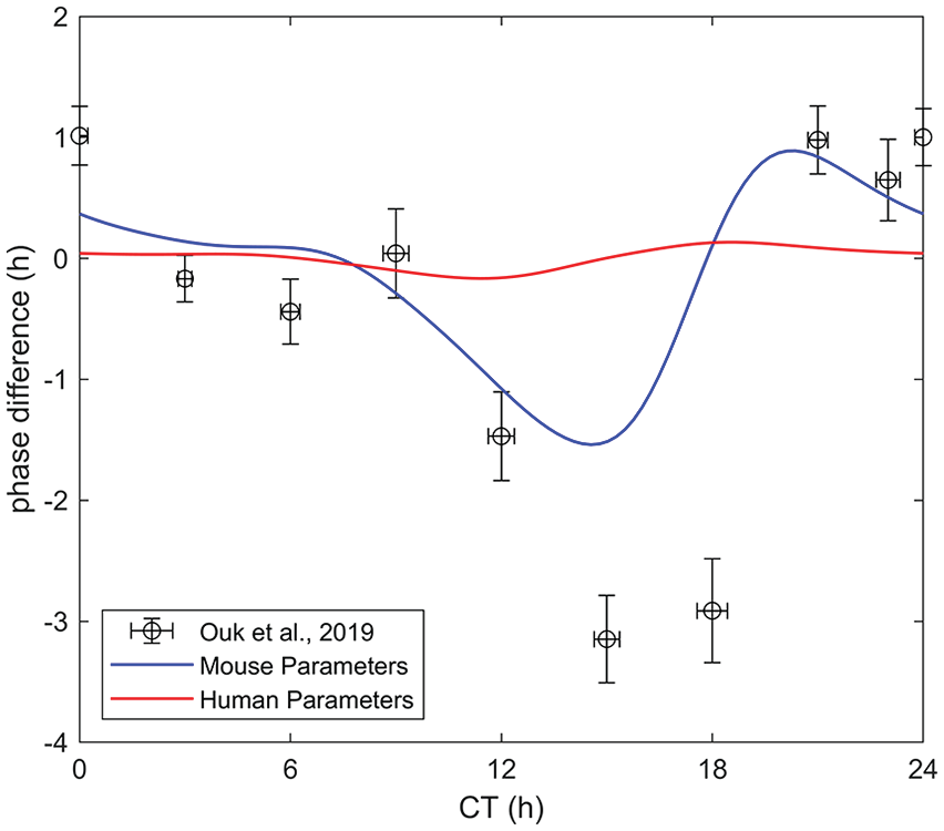
Comparison with experimental data (Ouk et al., 2019): The model parameters determined from the fit in Figure 1 are valid for a C57BL/6J mouse—The mice used in Ouk et al. (2019) are on a CBA × C57BL/6J background. As a result, the model does not have good agreement with the data especially in the phase delay region near CT 15. Abbreviation: CT = circadian time.
Local Sensitivity Analysis
It is well known that there is a great degree of intrinsic variability in the wild-type mouse free-running periods under both DD and LL. Some reasons for the intervariability between mice have been determined, such as sourcing from different labs (Capri et al., 2019), exposure to different wavelengths of light (Hofstetter et al., 2005) or even different types of white light (Alves-Simoes et al., 2016), and measuring the periods at different times in the mouse’s life cycle (Possidente et al., 1995). Even with these factors controlled, there is still significant variability between mice within the same environment. For these reasons, the parameters provided in this study should also include a range of possible numerical values.
First, we performed a local sensitivity analysis of the mouse model using a central finite difference method with a one-at-a-time (OAT) approach (Saltelli et al., 2008) to deduce the most significant parameters. For a parameter
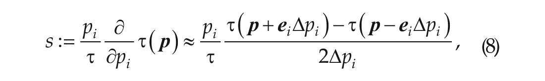
where
Using Equation 8, we perturbed each parameter
Period sensitivities
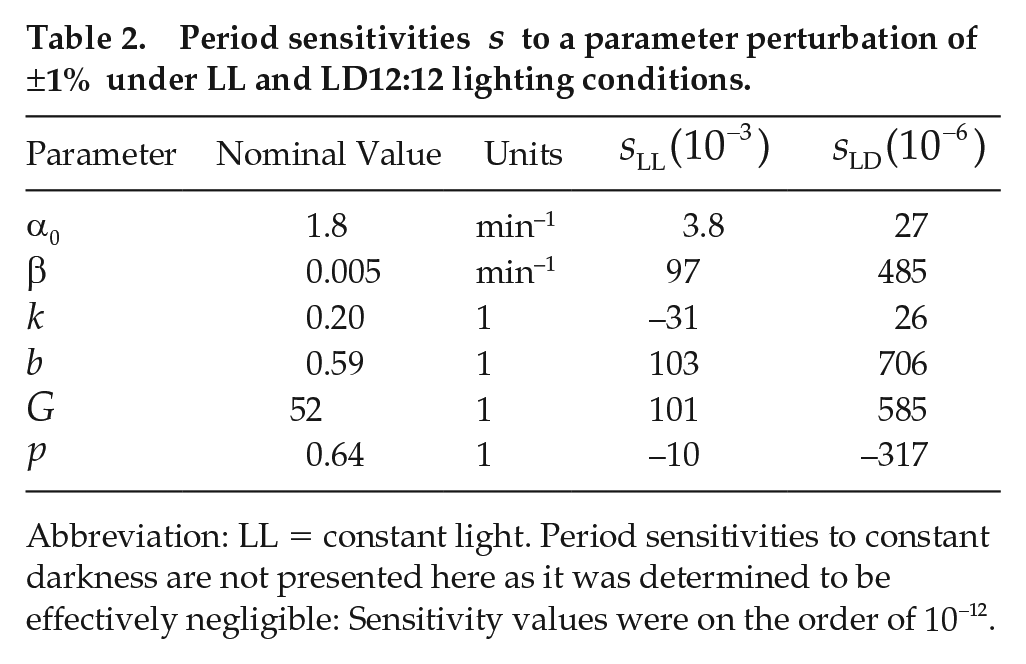
Abbreviation: LL = constant light. Period sensitivities to constant darkness are not presented here as it was determined to be effectively negligible: Sensitivity values were on the order of
We plot the model periods under LL, LD, and DD in Figure 5 for each perturbed parameter, up to variations of 25%. As reflected in Table 2, the period in LD and DD does not change appreciably under perturbations. The most relevant parameters that affect the period are
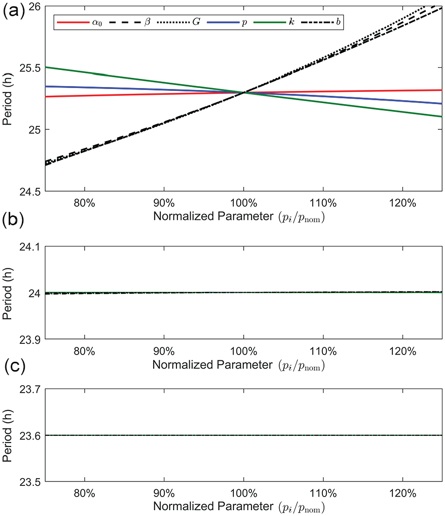
Model period under different lighting conditions: (a) LL, (b) LD12:12, and (c) DD by perturbing each model parameter by
The sensitivity analysis conducted suggests that the periods in LL are particularly sensitive to changes in the parameters
We also demonstrate the effects of varying
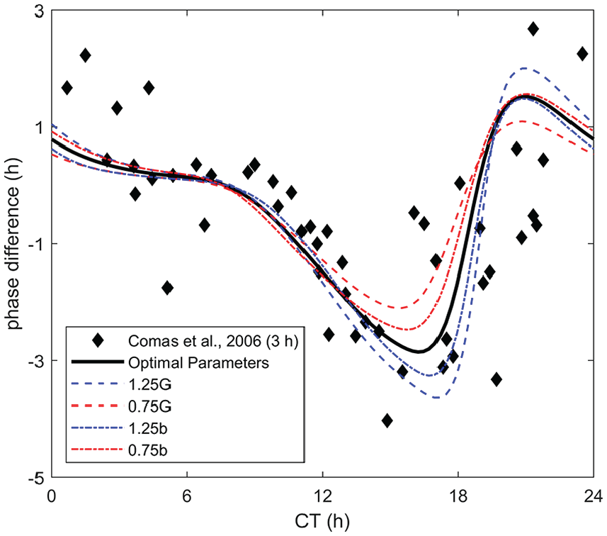
Comparison between a 3-h pulse phase response curve from Comas et al. (2006) with the optimal parameters and perturbations of the parameters
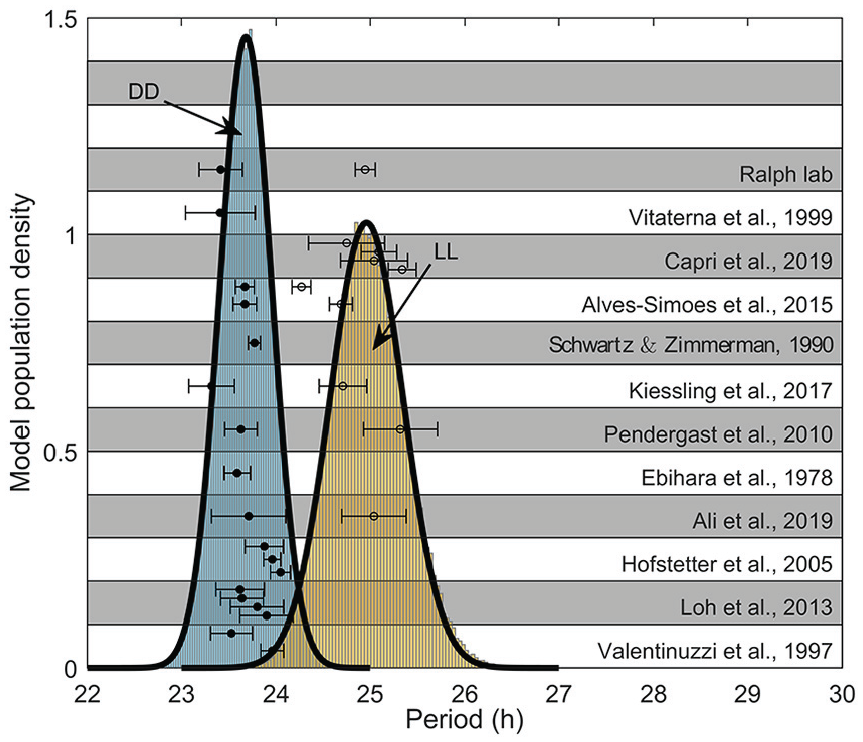
Period determined by model simulation under DD (blue histogram) and LL (yellow histogram) assuming a normal distribution for parameters
Parameter Variability
To determine the ranges for the key parameters, we re-fit with available data in the literature. We collected a wide range of studies, sourced from 12 different labs that reported the DD and/or LL periods of the C57BL/6 mouse. We calculated the total mean and standard deviation by combining the reported standard deviations and means from each data set
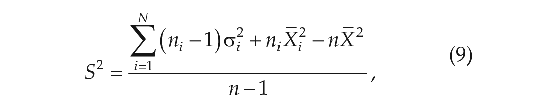
where
The parameter variability was determined as follows. First, the parameters were re-fit so that the observed period in LL was equal to the average experimental period in LL,
The best coefficients of variation were determined to be
In Table 3, we present the mean and standard deviation for the periods under DD and LL, along with the values of the mean and standard deviation for the model parameters,
Mean period
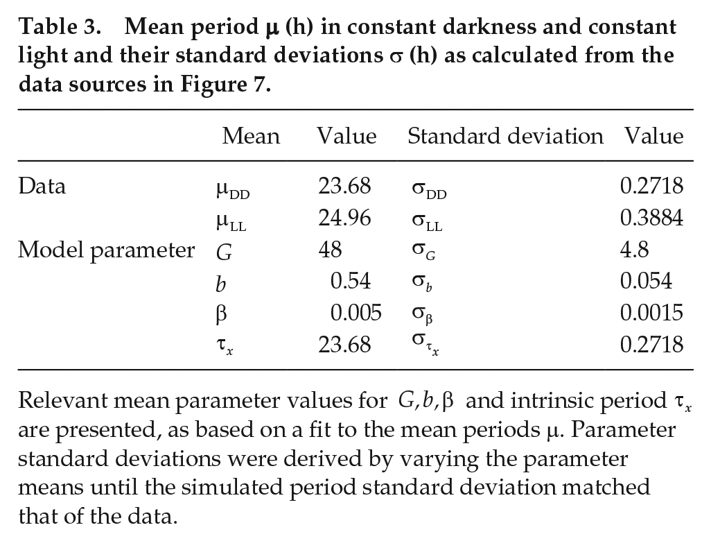
Relevant mean parameter values for
Applications
Maximal Phase Response
One use of the mouse model is to search for interesting protocols that result in large or maximal phase shifts. Previous empirical studies have investigated some aspects of inducing this behavior (Comas et al., 2006) but were restricted by the feasibility of large-scale experimentation in deducing the optimal protocol. Thus, we employed our mouse model, in silico, to design and report the optimal protocols of how to achieve maximal peak-to-peak amplitude, advance, and delay.
To determine the ideal light stimulus to induce the maximal peak-to-peak amplitude, advance, and delay, we fixed the light intensity at each chosen lux level (Table 4) and allowed for variation of light ON–OFF switching times, for
Largest peak-to-peak amplitude of a phase response curve (∆ (h)), largest phase advance (+∆ (h)), and largest phase delay (–∆ (h)) as calculated through an optimization procedure of switching times for light stimuli for varying light intensities (lx).
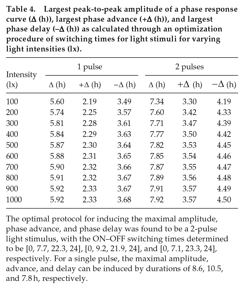
The optimal protocol for inducing the maximal amplitude, phase advance, and phase delay was found to be a 2-pulse light stimulus, with the ON–OFF switching times determined to be [0, 7.7, 22.3, 24], [0, 9.2, 21.9, 24], and [0, 7.1, 23.3, 24], respectively. For a single pulse, the maximal amplitude, advance, and delay can be induced by durations of 8.6, 10.5, and 7.8 h, respectively.
Our convention for the ON–OFF switching times is that light is ON at 0, OFF at the subsequent time, and this alternates as ON/OFF until the end of the stimulus where the light must be switched off so the simulation can be run in DD.
We restrict the maximal possible length of time of the stimulus to be 24 h. Within this time, we are able to provide any kind of stimulus (e.g., 2 pulses, 5 pulses). Note that this linear representation is not meant to be reflective of the circular clock but instead is a mechanism of representing multiple pulses of specific lengths and separations, which start from determined appropriate CTs in PRC experiments. As a concrete example, let us assume that the experimentalist constructing PRCs has determined the appropriate CTs. Then, say at CT 0, they implement our protocol,
For a number of pulses
It has been reported in previous studies on C57BL/6J-OlaHsd mice (Comas et al., 2006) and on humans (Dewan et al., 2011) that increasing duration is more effective in inducing phase changes of the circadian clock than that of increasing light intensity. We can see a similar result in our mouse model (Figure 8): the effect of light intensity on inducing phase shifts does cause some noticeable change, but the duration, and more specifically the pattern of light stimulus, is more effective.
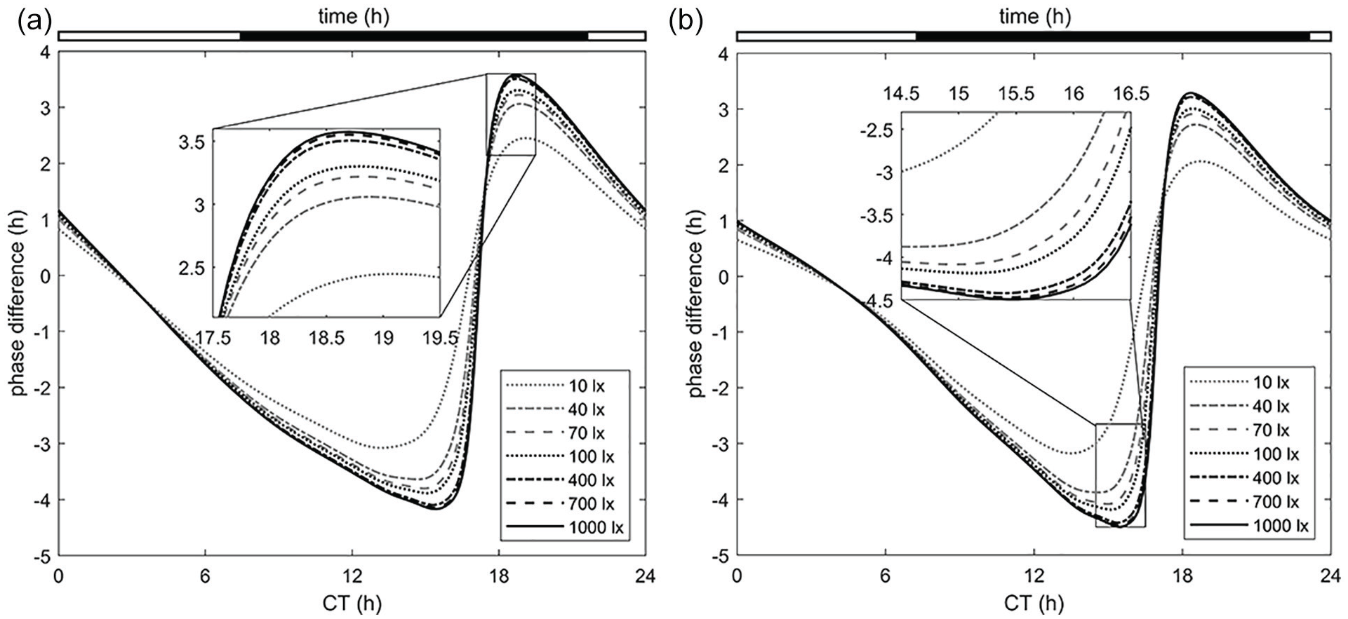
Phase response curves for varying light intensities using the optimal protocols (given above each panel) for (a) maximum advance and for (b) maximum delay. The optimal protocols for inducing maximal advance and maximal delay are the sets of ON–OFF switching times [0, 9.2, 21.9, 24] and [0, 7.1, 23.3, 24], respectively. Abbreviation: CT = circadian time.
The mouse study (Comas et al., 2006) only examined experimentally different durations of 100 lx single pulses and concluded the optimal duration for inducing the maximal amplitude is 9 h. Our model confirms that around 8.5 to 9 h indeed result in the maximal amplitude for a single pulse; however, it instead suggests that the 2-pulse protocol [0, 7.1, 23.3, 24] is more effective overall.
Comparison With a Mutant Mouse
We emphasize that the fit model parameters (Table 1) are specifically for the C57BL/6 mouse—Other mice or mutant strains that alter or possibly influence the circadian clock would not correlate well with the model parameters. One example of this is the casein kinase 1 epsilon deficient (CK1
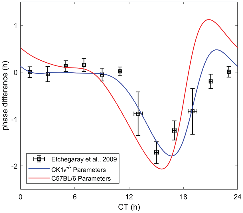
Phase response curve comparison between experimental data from Etchegaray et al. (2009) for the CK1
Discussion
Our results have revealed that there is a clear difference between the parameters responsible for photic input in humans compared with the C57BL/6 mouse. This discrepancy in parameter values between mice and humans can be explained as follows. Experiments involving nocturnal rodents, especially mice, use low-intensity light because of their susceptibility to retinal damage at high light intensities compared with humans (Gonzalez, 2018). Nocturnal rodents are also significantly more sensitive to low-intensity light than humans, avoiding dim lights and being able to condition to low-intensity light signaling (Eckmier et al., 2016). While it has been shown that human circadian systems also undergo phase shifts to lower light intensities (e.g., 180 lx; Boivin et al., 1996), the phases only shift with a mean of ∼∼
We admit that the lux unit can be problematic because it is based on the perceived brightness correlated to the human visual system (Peirson et al., 2018), and thus lends to potential issues in experimental data (Alves-Simoes et al., 2016; Hofstetter et al., 2005) as discussed prior. However, the use of lux has been accepted as a standard in the field due to the wide availability of and easy access to lux meters. Furthermore, above saturation, the difference between rhodopsin and melanopsin spectral sensitivities should not affect the interpretation of experiments. Regardless, our model takes into account the effects of different types of artificial light and provides a range of suitable parameters using parameter variation that reliably reproduces the characteristic data and behavior.
We note that the parameter k was slightly lower in mice than in humans. Previous authors studying human PRCs determined that the parameter
The circadian modulation, communicated through parameter
We have presented a mouse model of the original human model developed by Kronauer (1990). The model parameters were fit to available mouse data from the literature. The model was validated against other sets of experimental data and compared against the human model. For the same protocol, the mouse parameters yielded a significantly better match with the data than that of the human parameters. Sensitivity analysis conducted revealed that the measured period is only affected by perturbations under LL lighting conditions. Due to the reported variability of periods across and within labs, the most relevant parameters affecting the period were varied and compared with data from a wide range of sources to deduce a range of values for the key parameters. Using the mouse model to search for the optimal protocol for inducing maximal amplitude, advance, and delay determined that a 2-pulse light stimulus of switching times [0, 7.7, 22.3, 24], [0, 9.2, 21.9, 24], and [0, 7.1, 23.3, 24], respectively, was best. To further validate this model, we propose that future studies attempt other light protocols, especially the 2-pulse protocol as suggested by the optimization. The application of the mouse model to the CK1
Footnotes
Acknowledgements
We appreciate the constructive feedback provided by the anonymous reviewers. A.R.S. acknowledges the support of the Natural Sciences and Engineering Research Council of Canada (NSERC): RGPIN-2019-06946.
Conflict of Interest Statement
The author(s) have no potential conflicts of interest with respect to the research, authorship, and/or publication of this article.