
Abstract
Phase response curves (PRCs) play important roles in the entrainment of periodic environmental cycles. Measuring the PRC is necessary to elucidate the relationship between environmental cues and the circadian clock. Conversely, the PRCs of plant circadian clocks are unstable due to multiple factors such as biotic/abiotic noise, individual differences, changes in amplitude, growth stage, and organ/tissue specificity. However, evaluating the effect of each factor is important because PRCs are commonly obtained by determining the response of many individuals, which include different amplitude states and organs. The plant root circadian clock spontaneously generates a spatiotemporal pattern called a stripe pattern, whereby all phases of the circadian rhythm exist within an individual root. Therefore, stimulating a plant root expressing this pattern enables phase responses at all phases to be measured using an individual root. In this study, we measured PRCs for thermal stimuli using this spatiotemporal pattern method and found that the PRC changed asymmetrically with positive and negative temperature stimuli. Individual differences were observed for weak but not for strong temperature stimuli. The root PRC changed depending on the amplitude of the circadian rhythm. The PRC in the young root near the hypocotyl was more sensitive than those in older roots or near the tip. Simulation with a phase oscillator model revealed the effect of measurement and internal noises on the PRC. These results indicate that instability in the entrainment of the plant circadian clock involves multiple factors, each having different characteristics. These results may help us understand how plant circadian clocks adapt to unstable environments and how plant circadian clocks with different characteristics, such as organ, age, and amplitude, are integrated within individuals.
Plants have a circadian clock, which enables them to adapt to diurnal environmental changes. The circadian clock interacts with plant physiological processes, such as flowering and photosynthesis (Dodd et al., 2014; Creux and Harmer, 2019). The circadian clock is entrained by environmental cycles, matching the timing of these physiological processes to environmental changes (Salomé and McClung, 2005; Webb et al., 2019). This entrainment mechanism is explained by a phase response curve (PRC), which represents the phase shift in response to environmental stimuli at each phase of the circadian rhythm (Johnson et al., 2003; Granada et al., 2009). Measuring the PRC is important for understanding the relationship between environmental cues and the circadian clock (Haydon et al., 2013; Davis et al., 2018; Mwimba et al., 2018). Conversely, the entrainment of the plant circadian clock is sometimes unstable (Okada et al., 2017). One factor contributing to this unstableness is the variation in the period of the plant circadian clock, which can occur due to biotic/abiotic noise, individual differences, growth stage, and organ specificity (Bordage et al., 2016; Kim et al., 2016; Muranaka and Oyama, 2016; Li et al., 2020). These factors may also affect PRC properties. In addition, the PRC depends on the amplitude of the circadian rhythm (Masuda et al., 2017). However, evaluating the effect of each factor on the PRC using traditional measurement methods is difficult because these methods determine PRCs by gathering the responses of many individuals (Fukuda et al., 2008). Hence, a method that can measure a precise PRC from one individual is needed.
The plant root circadian clock exhibits a spatiotemporal pattern, called a stripe pattern, which is generated by the phase reset of the root tip and root elongation and/or the differences in free-running periods along the root under constant conditions (Fukuda et al., 2012; Gould et al., 2018). In this pattern, each phase of the circadian clock (e.g., subjective day, subjective night) appears repeatedly as a stripe pattern. When a root with this pattern is stimulated, the phase response can be observed at each phase from an individual root. Therefore, measuring the PRC using a spatiotemporal pattern enables the effects of contributing factors on the unstableness of entrainment in the plant circadian clock to be evaluated.
In this study, we measured PRCs for thermal stimuli using this spatiotemporal pattern. We demonstrated that PRCs for thermal stimuli could be reconstructed from individual roots by measuring the PRC using the spatiotemporal pattern. To measure the PRC, the rhythm of Arabidopsis clock genes, CIRCADIAN CLOCK ASSOCIATED1 (CCA1) and TIMING OF CAB EXPRESSION 1 (TOC1) were evaluated using a luciferase reporter assay. We measured the PRCs thermal stimuli (30 min pulses, ±3 and ±10 C) because temperature change is the primal zeitgeber for plant roots. We compared the root PRCs for thermal stimuli in CCA1 and TOC1 because a previous study reported differences in the PRC for thermal stimuli in different clock genes (Michael et al., 2003a; Masuda et al., 2021). We also confirmed that changes in the PRC depend on the amplitude of circadian rhythms, as reported previously (Masuda et al., 2017). To observe differences in PRCs at different ages and positions, we applied the temperature stimuli twice, on days 7 and 14, as the roots grew during the measurement period. In addition, we performed a numerical simulation using the phase oscillator model for plant roots (Fukuda et al., 2012). Using this simulation, we investigated the effect of internal and measurement noises on the PRC because of the difficulty in distinguishing the effects of these factors in experiments.
Materials and Methods
Plant Materials and Experimental Methods
Transgenic Arabidopsis thaliana Col-0 CCA1::LUC and TOC1::LUC, which carry luciferase reporters driven by promoters of the clock genes CCA1 and TOC1, respectively, were used to monitor plant root circadian rhythms (Nakamichi et al., 2004; Uehara et al., 2019). Plants were grown on gellan gum-solidified Murashige-Skoog medium with 2% (w/v) sucrose and 0.1 mM luciferin on vertical plates (120 × 90 × 10 mm, three individuals per plate) under 12 h light (100 µmol m–2 s–1 of fluorescent white light): 12 h dark cycles at 22 ± 0.5 °C for 7 days. Bioluminescence was monitored by a sensitive EM-CCD camera (Hamamatsu Photonics KK, Japan) in a dark box with a Peltier device at 22 ± 0.1 °C for 17 to 21 days. Measurements were taken every 30 min, and the exposure time was set to 3 min for CCA1 and 10 min for TOC1. The image size was 512 × 512 pixels. The bioluminescence in each pixel was determined as a 2-byte datum (i.e., a value between 0 and 65,535). Thirty minutes of ±3 or ±10 °C stimulation was applied at 168 and 336 h (i.e., 7 and 14 days) after the beginning of the measurement in a single experiment. The experiments for each temperature stimulus and with CCA1::LUC and TOC1::LUC plants were performed once independently.
Data Analysis
Primary root bioluminescence was extracted from bioluminescence images by mask images, which were prepared manually (Suppl. Fig. S1). Bioluminescence at the same height was averaged. The bioluminescence data were normalized as follows:


where
The moving average was calculated to remove noise from the data, as follows:

where M is the window of the moving average. M was set to 12 to set the moving average window to 12 h.
To detect peak and trough bioluminescence, the slope

The moving average was set to W = 24. The peak point l of the bioluminescence oscillation is defined as the point at which
Denoting the time of the kth peak in the bioluminescence signal by tp(k), the period at the kth peak was defined as

In this study, the peak number k represents the root age starting from when the root emerged.
The phase θ at time t was defined as

Here, τ0 is the free-running period and τ0 = 28 h. Since the time from peak to trough bioluminescence was 14 h, the trough phase was θ = 14 of 28 × 2π rad.
Each pulse was administered at time tstim. For two consecutive peaks, tp(k) and tp(k + 1) that satisfy tp(k) ≤ tstim ≤ tp(k + 1), the phase shift Δθ induced by the pulse was calculated as

Phase shifts from the troughs were calculated in the same manner.
Normalized amplitude

where N is the same as in Equation 2.
The approximated curves were assumed to be

Each parameter of Equation 10 was determined by the sum maximization of
Numerical Simulation
Numerical simulations were performed using the coupled phase oscillator model, which has been suggested to reproduce the spatiotemporal pattern of the plant root circadian clock (Fukuda et al., 2012). The model is given by the following equations:
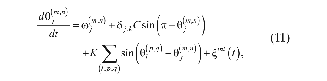

Here,
Results
Spatiotemporal Pattern in the Plant Root Circadian Clock
Figure 1a shows the time-space plot for the −10 °C stimuli. The root was growing throughout the experiment, and the root exhibited a stripe pattern, in which the phases of the circadian clock over several cycles exist simultaneously. Figure 1b shows the bioluminescence at the horizontal broken lines in Figure 1a. The circadian clocks at different heights oscillated in different phases (Figure 1b and Suppl. Fig. S2). The spatiotemporal pattern differed among individuals (Suppl. Fig. S3). The root near the hypocotyl was in the short period; the middle of the root was in the long period, and the root around the tip was in the short period (Suppl. Fig. S4). This position dependence of the root circadian clock period is similar to the result of a previous study (Gould et al., 2018; Greenwood et al., 2019). The period was short just after root emergence, was maximal after several cycles, and then gradually shortened (Suppl. Fig. S5). However, since the number of peaks was small at the tip of the root, when the peak number is large, the data might be more closely related to the hypocotyl than to the root tip. Some individual differences in period were also observed.
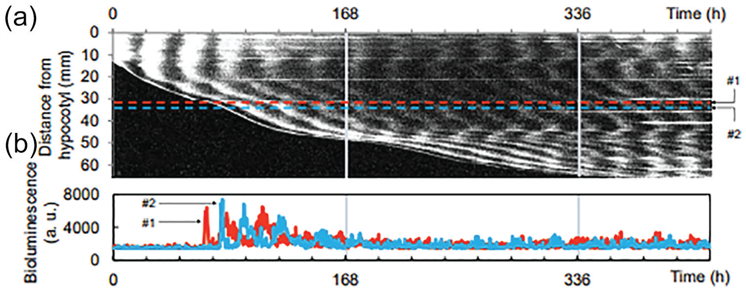
Stripe pattern in the plant root clock under constant dark conditions: (a) Time-space plot of the plant root clock. (b) Bioluminescence at the horizontal broken lines (#1, #2) in (a). The vertical lines at 168 and 336 h indicate the −10 °C stimuli.
PRCs for Thermal Stimuli
Figure 2 shows the PRCs for temperature stimuli in CCA1 and TOC1. The shape of the PRCs differed with different stimuli. Larger temperature changes induced stronger responses for each positive and negative thermal stimuli. The PRC for heating stimuli showed a larger amplitude than that for cooling stimuli. The stable point of the PRC for +10 °C was the middle of the day phase. In contrast, the stable point for −10 °C was the middle of the night phase. The stable point for −3 °C was almost the same as that for −10 °C, while that for +3 °C was close to the stable point for negative temperatures rather than that for +10 °C. These results indicate that the PRCs for thermal stimuli depend on their magnitude; the PRCs asymmetrically changed from positive to negative temperature stimuli. These changes are consistent with a previous study (Masuda et al., 2021). The PRCs in CCA1 were the opposite phase to those in TOC1, as CCA1 and TOC1 oscillate in opposing phases. Therefore, our results indicated that there were small differences between CCA1 and TOC1 in root PRCs. On the contrary, previous studies have reported PRC differences for temperature stimuli between genes in individual roots (Michael et al., 2003a; Masuda et al., 2021). In these studies, PRC was measured under constant light conditions, and in the present study, it was measured under constant dark conditions. Therefore, the presence or absence of light may affect the responsiveness to temperature stimuli.
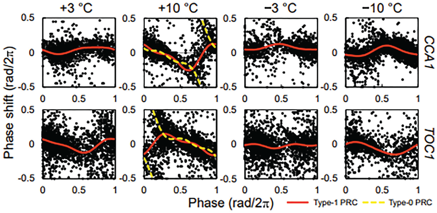
PRCs for temperature stimuli. Each PRC represents the sum of three individual roots. The solid lines indicate the approximate curves assuming type 1 PRCs. In PRCs for +10 °C, the approximate curves assuming type 0 PRCs (broken lines), described as
Individual Differences in PRCs
Figure 3 shows the PRCs for +3 and +10 °C in individual plants. These results indicate that a PRC can be reconstructed from only one individual root when measuring the PRC using the stripe pattern. Individual PRCs for the same simulation have a similar stable point and amplitude. However, unstable points of PRCs for +3 °C were not identical, as there were some individual differences around θ = 0.3 – 0.4 (rad/2π). There was no significant difference in peak number and position between No. 1 and No. 2 (Suppl. Fig. S6). This indicates that there are individual differences in the entrainment properties of the plant circadian clock. Conversely, PRCs for +10 °C exhibited smaller differences than those for +3 °C. Therefore, individual differences in the PRC may depend on the strength of the stimulus and may become more unstable with a weaker stimulus.
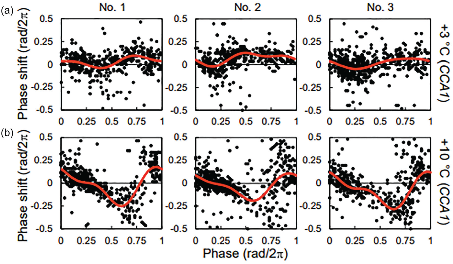
PRCs in individual roots for the +3 °C (a) and +10 °C (b) stimuli. The red lines indicate the approximate curves. The PRCs for +3 °C and +10 °C at the same number were obtained from the different individuals. Abbreviations: PRCs = phase response curves; CCA1 = CIRCADIAN CLOCK ASSOCIATED1.
Amplitude-dependent Change in the PRC
In PRCs for +10 °C, there was a large distribution in the phase shift around the unstable point (Figure 2). A previous study reported that the PRC changes from type 1 to type 0 depending on the decreased amplitude of circadian rhythms (Masuda et al., 2017). Therefore, the rhythm amplitude can also influence the PRCs in plant roots. Figure 4a and Supplementary Figure S7 show the PRC for +10 °C in CCA1 in high- and low-amplitude states. The PRC in the high-amplitude state was type 1, which was continuous in all phases. Conversely, the PRC in the low-amplitude state was type 0, with a discontinuous point. The stable and unstable points of the PRCs were very similar. The phase shifts around the stable point were similar between the high- and low-amplitude states. However, the phase shifts around the unstable point were continuous in the high-amplitude state but discontinued in the low-amplitude state. Figure 4b shows the phase shift against the change of amplitude. The PRC amplitude increased with decreasing amplitude and rapidly increased around 0.1 amplitude. These results are similar to those reported previously (Masuda et al., 2017). The amplitude-dependent change in the PRC was also observed in TOC1 (Figure 4c and 4d and Suppl. Fig. S7). The high-amplitude state tended to be in the lower root, but the high- and low-amplitude states were distributed throughout the roots (Suppl. Fig. S8A). There was no significant difference in the peak numbers between both states (Suppl. Fig. S8B). The sample frequencies were higher for peak numbers 4 and 11 than for the other peak numbers because the peak numbers of the preexisting regions at the beginning of the measurement were aligned, and the first and second stimuli correspond to the 4th and 11th peaks of these regions, respectively (Figure 1). The previous study explained that this PRC change is caused by the desynchronization of circadian rhythms between cells (Masuda et al., 2017). In the current study, the size of one pixel in the image is about 230 μm, and time-series data at a certain height are the average of several pixels. The size of cells in the Arabidopsis root is about 10 to 100 μm; therefore, one time-series is the sum of at least 100 cells (Seki et al., 2018). Moreover, phase-dependent response of amplitudes were also observed (Suppl. Fig. S9). These changes in amplitude correspond to the prediction based on multicellularity, where amplitude increases at the stable point of the PRC and decreases at the unstable point (Fukuda et al., 2013). Therefore, the change in PRC depending on amplitude is related to the desynchronization of circadian rhythms among cells. A previous study also reported that the PRC under high-amplitude conditions coincides with that at the cellular level (Masuda et al., 2017). Therefore, the root PRC should be measured at a high amplitude to obtain accurate entrainment properties.
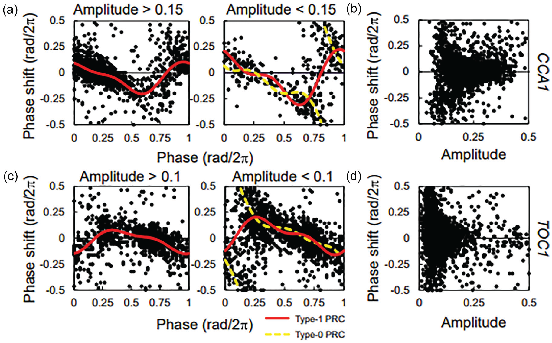
Amplitude-dependent changes in PRCs for +10 °C in CCA1 (a) and (b) and in TOC1 (c) and (d). (a) and (c) indicate PRCs in high-amplitude (left side) and low-amplitude (right side) states. The solid and broken lines indicate the approximate curves assuming type 1 and type 0 PRCs, respectively. (b) and (d) indicate the change in magnitude of phase shift depending on the change in amplitude. Abbreviations: PRCs = phase response curves; CCA1 = CIRCADIAN CLOCK ASSOCIATED1; TOC1 = TIMING OF CAB EXPRESSION 1.
Position- and Age-associated Changes in PRCs
In this study, the thermal stimuli were applied on days 7 and 14 after the start of the measurement period. The root grew gradually during the measurement period. Therefore, the obtained PRCs included the responses in the root at a certain age and position. Figure 5 shows the change in PRCs for +3 and −10 °C in CCA1 associated with root age and position. The peak number represents the root age, and the distance from the hypocotyl represents the root position. In the upper part (distance ≤ 150 pixels) of the young root (peak number ≤ 6), the amplitude of the PRC was larger than that in the other conditions. Conversely, the PRC in the lower part of the old root was similar to that in the upper part of the old root and the lower part of the young root. The PRCs in the upper part of the young roots were more sensitive than those in the other conditions; however, the amplitude in these roots was not necessarily smaller than that in the others (Suppl. Fig. S10). In other conditions, the number of data points was too small to evaluate the differences correctly in some conditions (e.g., +3 °C and −10 °C in TOC1), but the tendency did not differ significantly (Suppl. Figs. S11 and S12). Therefore, root age and position may affect the instability of entrainment independently of the amplitude.
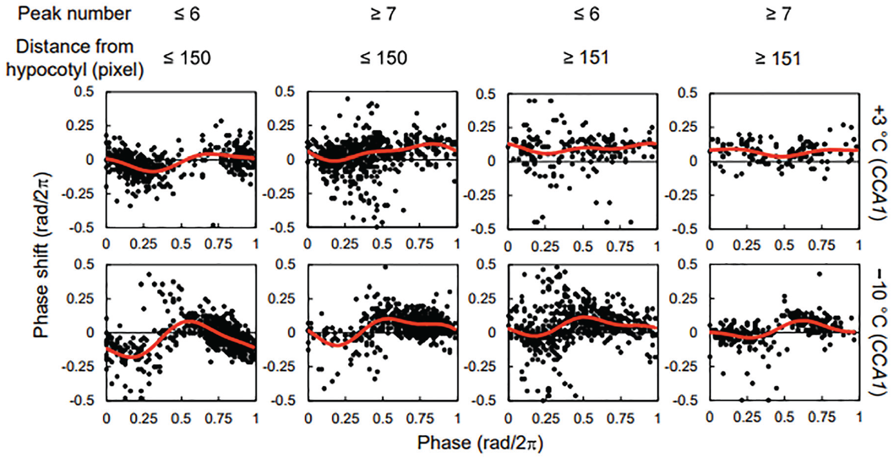
Position- and age-associated changes in PRC for +3 and −10 °C stimuli in CCA1. The red lines indicate the approximate curves. One pixel is about 0.23 mm. Abbreviations: PRCs = phase response curves; CCA1 = CIRCADIAN CLOCK ASSOCIATED1.
Effect of Internal and Measurement Noises on the PRC
The stripe pattern was reproduced by numerical simulations (Suppl. Fig. S13). Noise blurred the rhythms, but the spatiotemporal pattern was still observed. The +10 °C stimuli were applied on days 7 and 14 of the simulation. The cells were largely synchronized after the second stimulus. Figure 6 shows the PRCs for +10 °C in simulations with and without noise. In the noiseless condition, the PRC was less distributed than was observed experimentally. However, the PRC was unstable at the unstable point, despite the absence of noise. This could be due to variation in natural frequency in each cell. The PRC in the measurement noise condition was more distributed than that in the noiseless condition at all phases. Conversely, the PRC in the internal noise condition was less distributed at the stable point but more distributed at the unstable point. This difference indicates that the internal noise affected the synchronization among cells. The PRC in the condition with measurement and internal noises was the most distributed and appeared similar to that obtained experimentally.
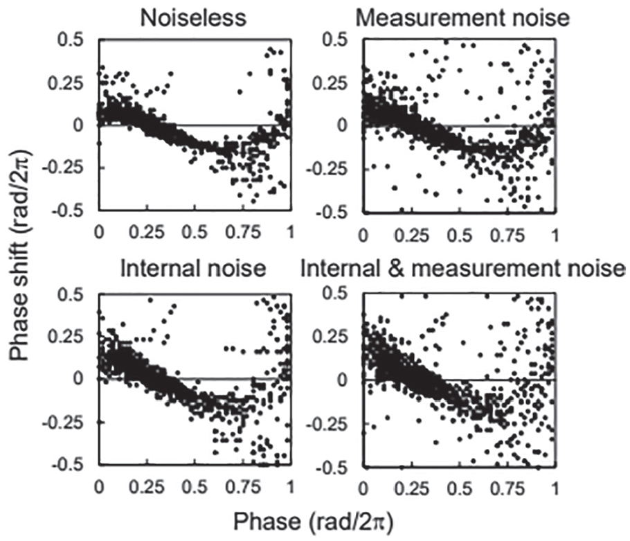
Phase response curve in simulation with/without internal and measurement noises.
Discussion
In this study, we measured plant root PRCs for thermal stimuli from individual roots using a spatiotemporal pattern. Previous studies have reported that the plant circadian clock in leaves is also spontaneously desynchronized (Wenden et al., 2012; Muranaka and Oyama, 2016). Other studies have demonstrated that desynchronization among cells can be caused by artificial light control (Fukuda et al., 2013; Seki et al., 2015). Hence, this method of measuring PRCs can be applied to other plant organs, such as the leaf or stem, by artificially controlling the environment. Organ and tissue specificity of the plant circadian clock has been previously reported (Endo et al., 2014; Takahashi et al., 2015). Therefore, this method may elucidate the organ/tissue specificity on entrainment properties and the instability of entrainment depending on these characteristics.
In previous studies, the spatiotemporal pattern of roots has been explained by the phase resetting at the root tip and period differences at different positions (Fukuda et al., 2012; Gould et al., 2018). In the present study, we also found that the period depended on the position and age of the root; the period was shorter in the upper part of the root and at the root tip and was longer in the middle as shown in the previous study (Suppl. Figs. S4 and S5 in the present study; Gould et al., 2018). In this case, a root pattern convex to the right appears, and similar patterns were partially observed in the present experiment (Suppl. Fig. S3). On the contrary, a stripe pattern from the upper left to the lower right was also observed (Suppl. Fig. S3). To explain this pattern by the period changes, it is necessary that the period becomes longer immediately after the root development, but in the present results, a short period was observed. These results indicate that this kind of stripe pattern is caused by the phase resetting at the root tip. Therefore, period differences and phase resetting at the root tip may be involved in the spatiotemporal pattern of roots. To measure the response for the entire phase using this pattern, a more accurate spatiotemporal pattern prediction may be necessary. In addition, stimulations were given on days 7 and 14, and the responses were measured from each date in this experiment. When the stimulus is weak, there is sufficient phase variation even with the second stimulus (Suppl. Fig. S2), but the phase bias may increase when the stimulus is strong. Therefore, when measuring multiple responses in one experiment, it may also be necessary to consider the effect of stimuli on spatiotemporal patterns.
Individual differences in PRCs, as shown in Figure 3, may be due to several factors. Here, plants differed in terms of period and PRC depending on the root position and age (Figure 5 and Suppl. Figs. S4 and S5). The rate of root elongation also varies between individuals. These differences may induce variation in the phase response. Figure 4 shows that the PRCs changed depending on changes in amplitude. This change was large at the unstable point. The individual differences shown in Figure 3 were also notable at the unstable point. Thus, differences in amplitude may be a contributing factor to individual variation. Otherwise, individual variations in phase response properties may exist, similar to variations in the period of circadian rhythms (Michael et al., 2003b). To verify these differences, it is necessary to compare the PRCs by sorting out all the factors (amplitude, age, position, and other factors) in the same individual. However, even with the method used in this study, it remained difficult to obtain sufficient data points (Suppl. Figs. S11 and S12). Therefore, further improvement of the method is needed to identify the factors that contribute to individual differences.
This study highlights several contributing factors to the instability of entrainment; however, other factors can also be considered. PRCs for positive and negative temperature stimuli followed opposite patterns and were not symmetrical. Thus, thermal noise can cause phase shifts even if the value of the noise is zero on average. Therefore, the degree of thermal noise may affect the stability of the circadian clock. Some secondary roots appear from the primary roots in Arabidopsis thaliana (Suppl. Fig. S1A). In Figure 1a, the horizontal white lines at 10 and 20 mm on the vertical axis indicate the emergence of secondary roots. The root circadian clock was reset to subjective dusk at the root tip (Fukuda et al., 2012; Voß et al., 2015). Thus, the pattern of secondary root generation may also be related to the spatiotemporal pattern of the circadian clock in plant roots (Seki et al., 2018). Several studies have reported differences in entrainment properties depending on the clock genes (Michael et al., 2003a; Flis et al., 2016). Therefore, differences between clock genes may disturb entrainment through the clock gene network. A few studies have reported the interaction of circadian rhythms between cells and organs (Fukuda et al., 2012; Takahashi et al., 2015; Gould et al., 2018; Greenwood et al., 2019). Considering the different entrainment properties between cells and organs, coupling is important for the entrainment of circadian rhythms.
In this study, we demonstrated that the PRC could be measured using the spatiotemporal patterns of the plant root circadian clock. In addition, our results revealed that there are various factors involved in the instability of entrainment of circadian rhythms and showed their characteristics. These results may help us understand how the plant circadian clock adapts to unstable environments, and our method may also be useful in understanding how plant circadian clocks with different characteristics, such as organ, age, amplitude, are integrated within individuals.
Supplemental Material
sj-docx-1-jbr-10.1177_07487304211028440 – Supplemental material for Unstable Phase Response Curves Shown by Spatiotemporal Patterns in the Plant Root Circadian Clock
Supplemental material, sj-docx-1-jbr-10.1177_07487304211028440 for Unstable Phase Response Curves Shown by Spatiotemporal Patterns in the Plant Root Circadian Clock by Kosaku Masuda and Hirokazu Fukuda in Journal of Biological Rhythms
Footnotes
Acknowledgements
We are grateful to Dr. Kazuya Ukai for advising on the measurement method and the simulation and Prof. Norihito Nakamichi for providing the CCA1:: LUC and TOC1:: LUC plants. This study was partially supported by Grants-in-aid for Scientific Research (No. 18J20079 to K.M., 20H00423, 20H05424, 20H05540 to H.F.) provided by the Ministry of Education, Science, Sports, and Culture in Japan.
Author Contributions
K.M. performed the experiments, analyzed the experimental data, and performed the simulation. K.M. and H.F. designed the research, wrote the manuscript, discussed the results and implications, and reviewed the manuscript.
Conflict of Interest Statement
The author(s) have no potential conflicts of interest with respect to the research, authorship, and/or publication of this article.
NOTE
Supplementary material is available for this article online.
References
Supplementary Material
Please find the following supplemental material available below.
For Open Access articles published under a Creative Commons License, all supplemental material carries the same license as the article it is associated with.
For non-Open Access articles published, all supplemental material carries a non-exclusive license, and permission requests for re-use of supplemental material or any part of supplemental material shall be sent directly to the copyright owner as specified in the copyright notice associated with the article.