A Computational Error and Restricted Use of Time-series Analyses Underlie the Failure to Replicate period -Dependent Song Rhythms in Drosophila

Abstract

From 1980 to 1991, Kyriacou, Hall, and collaborators (K&H) reported that the Drosophila melanogaster courtship song has a 1-min cycle in the length of mean interpulse intervals (IPIs) that is modulated by circadian rhythm period mutations. In 2014, Stern failed to replicate these results using a fully automated method for detecting song pulses. Manual annotation of Stern’s song records exposed a ~50% error rate in detection of IPIs, but the corrected data revealed period-dependent IPI cycles using a variety of statistical methods. In 2017, Stern et al. dismissed the sine/cosine method originally used by K&H to detect significant cycles, claiming that randomized songs showed as many significant values as real data using cosinor analysis. We first identify a simple mathematical error in Stern et al.’s cosinor implementation that invalidates their critique of the method. Stern et al. also concluded that although the manually corrected wild-type and per^L mutant songs show similar periods to those observed by K&H, each song is usually not significantly rhythmic by the Lomb-Scargle (L-S) periodogram, so any genotypic effect simply reflects “noise.” Here, we observe that L-S is extremely conservative compared with 3 other time-series analyses in assessing the significance of rhythmicity, both for conventional locomotor activity data collected in equally spaced time bins and for unequally spaced song records. Using randomization of locomotor and song data to generate confidence limits for L-S instead of the theoretically derived values, we find that L-S is now consistent with the other methods in determining significant rhythmicity in locomotor and song records and that it confirms period-dependent song cycles. We conclude that Stern and colleagues’ failure to identify song cycles stems from the limitations of automated methods in accurately reflecting song parameters, combined with the use of an overly stringent method to discriminate rhythmicity in courtship songs.

From 1980 until the early 1990s, a series of studies from Kyriacou, Hall, and their collaborators (K&H) demonstrated that a Drosophila melanogaster male’s courtship song, produced by the male’s wing vibration, included a cycling component (Kyriacou and Hall, 1980, 1982, 1984, 1985, 1986, 1989; Kyriacou et al., 1990; Zehring et al., 1984; Hamblen et al., 1986; Yu et al., 1987; Wheeler et al., 1991). The interpulse interval (IPI) was shown to oscillate in wild-type males with a period of ~60 s and was modulated in a predictable fashion by the circadian rhythm period mutants (Konopka and Benzer, 1971; Kyriacou and Hall, 1980, 1986). The work was performed with light-sensitive oscillographic paper records of the song; IPIs were measured with a ruler and pencil. Even this laborious approach was feasible only if IPIs were binned into consecutive 10-s segments of real time and a mean IPI then computed for each bin, which usually contained 20 to 50 individual IPIs. The mean IPIs for songs of several minutes’ duration were then analyzed using an iterative sine-wave fitting procedure, very similar to the formal cosinor method (Refinetti et al., 2007), in order to find the best period, amplitude, and phase by reducing sums of squares. Spectral analysis was also used to generate an initial period for the sine-wave so that the iterative curve-fitting procedure would not be trapped in a local minimum (Kyriacou and Hall, 1989; Kyriacou et al., 1990). Alt et al. (1998) were able to independently reproduce the K&H song findings with per mutants, as was Crossley (1988), although somewhat unexpectedly (see Kyriacou and Hall, 1989). Ritchie et al. (1999) replicated and extended K&H’s playback experiments, which showed that species-specific rhythmic songs enhance female mating (Kyriacou and Hall, 1982, 1986; Greenacre et al., 1993).

Stern (2014) used a fully automated method to detect IPIs that was claimed to be highly efficient in detecting song pulses (Arthur et al., 2013) but could not confirm the existence of song rhythms, either by binning or by the analysis of nonbinned individual IPIs (Stern, 2014). He suggested that the results obtained in the 1980s were artifacts of the methodology used, as temporal binning imposes limits on the frequencies that can be sampled. Indeed, binning using mean IPIs in 10-s bins can detect only minimum periods of twice the bin size (Nyquist value, so 20 s) and half the length of the data set, which was set to 150 s, as most courtships lasted for 200 to 400 s. Kyriacou et al. (2017) visually and acoustically inspected the raw song records of Stern (2014) and observed that the automated detection method was only ~50% accurate. A number of other experimental shortcomings were observed in Stern’s data, particularly that nearly all song recordings, apart from the per^L genotype, were very poor in terms of vigor, with large gaps between bursts of song, making any analysis of song rhythms pointless. Kyriacou et al. (2017), using the operational criteria they had employed in the 1980s, reanalyzed Stern’s raw song records and limited the analysis to only those flies that exhibited robust singing. This included 25% of wild-type and almost all per^L songs. Cosinor analysis of binned mean IPIs revealed a significant difference between wild-type and mutant songs, with mean periods almost identical to those originally published by K&H (Kyriacou and Hall, 1980). These results were supported by 2 independent spectral analyses, Lomb-Scargle (L-S) and CLEAN (Roberts et al., 1987), as well as autocorrelation. Furthermore, when the L-S algorithm was also applied to the unbinned IPIs, while the most significant periods were nearly always found in the very short, <1-s period range (as in Stern, 2014), comparing the peak periods in each song between per^L and wild type in the 20- to 150-s range matched almost exactly those observed with the binned data, again supporting K&H’s original observations (Kyriacou et al., 2017).

Stern et al. (2017) have acknowledged that Stern’s (2014) automated IPI detection was inefficient but nevertheless insisted that unless an individual song’s mean IPI pattern is significant by L-S spectral analysis, any peak period in the spectral plot is simply “noise.” Binned mean IPI data sets are necessarily short, with 30 to 40 data points representing 300 to 400 s of courtship time. Spectral analysis imposes extremely high significance thresholds for short time series that can be satisfied only by almost perfect sinusoids, so such methods are appropriate for hundreds if not thousands of data points (Logan and Rosenberg, 1989). Consequently, techniques such as cosinor, used for decades by chronobiologists, have been used to analyze shorter time series (Cornelissen, 2014). It was therefore extremely surprising that Stern et al. (2017) also claimed that the cosinor method generated as many (in fact more) significant periods in randomized song data as in the real data, leading them to dismiss all of the original K&H work that was based on cosinor analysis of mean IPIs.

Stern et al. (2017) therefore restricted their reanalysis of the songs manually annotated by Kyriacou et al. (2017) to unbinned IPIs. Using L-S, they generated a marginal (p = 0.057) difference in the expected direction between per^L and wild-type periods, compared with the same analysis on these data performed by Kyriacou et al. in which a more robust statistical difference between the genotypes was observed (Kyriacou et al., 2017). In addition, Stern et al. (2017) recorded a large number of new per^L and wild-type songs, and using a modified version of their pulse detection algorithm claimed to identify ~80% of IPIs, they again showed the predicted but marginal (p = 0.06) difference between per^L and wild-type songs. In both cases, Stern et al. suggested that as most of the peak periods within the individual data in the 20- to 150-s range are not significant using L-S, then these peaks must represent noise.

Here, we first demonstrate that a simple error in Stern et al.’s code has incorrectly led them to conclude that the cosinor method generates too many false positives. We also compare the L-S algorithm using conventional locomotor data to 3 other time-series methods and find that it is highly conservative. By recomputing L-S confidence limits based on randomizations rather than using the theoretically derived values, we find that L-S now agrees with the 3 other methods in assigning significance to individual locomotor records. We apply this modified L-S to the song data and observe significance in the majority of individual records and period-dependent differences. We then apply the CLEAN spectral procedure to the songs and again confirm the significance of individual song rhythms and their period dependence. Finally, we observe that Stern et al.’s (2017) amended automated pulse detection method for their new set of song recordings, although improved from that used in Stern’s previous study (Stern, 2014), still generates an unacceptable error rate higher than claimed. We conclude that in both binned and unbinned IPIs, period-specific song rhythms can be detected in Stern’s (2014) data, thereby further supporting the original song cycle work of the 1980s.

Methods and Materials

MATLAB Analyses

We obtained the MC CLEAN V2.0 package from D. Heslop, a MATLAB implementation of CLEAN (Baisch and Bokelmann, 1999) that was modified to include a robust statistical framework (Heslop and Dekkers, 2002). Confidence limits of 95% and 99% were generated by a randomization procedure that we reimplemented to take advantage of the parallel computing toolbox functions available within newer versions of MATLAB. Implementations of L-S and cosinor were obtained from the MATLAB FileExchange service; the WAVOS package (Harang et al., 2012) allowed us to implement Morlet wavelet analyses for equally spaced data sets, and autocorrelation was performed using built-in MATLAB functions. Analyses were run on the Leicester University SPECTRE high-performance computing cluster.

Song Analysis

The data reexamined here represents the song records from Stern (2014) that were manually annotated and analyzed (Kyriacou et al., 2017; Stern et al., 2017). The whole data set of 25 wild-type and 14 per^L songs was analyzed with CLEAN to resolve periods down to 80 ms, the latter reflecting the minimum possible cycle of approximately twice the average IPI, as well as down to 0.4 s to match analyses performed using L-S (Kyriacou et al., 2017; Stern et al., 2017). The annotated individual IPI records were analyzed without binning through the CLEAN algorithm using MATLAB with 500 iterations of CLEAN and 1000 randomizations to generate confidence limits. We had not used CLEAN on unbinned IPIs in Kyriacou et al. (2017) because of the excessive time (12-24 h) previous implementations took to analyze a single song on a laptop at high resolution (Kyriacou et al., 2017). Manual analysis of Stern et al.’s new songs was performed as described in Kyriacou et al. (2017).

Locomotor Analysis

Eurydice pulchra were collected at spring tides between June and September 2015 from a beach near Bangor, taken to Leicester, and injected with a control construct (RNAi against YFP), then immediately placed into constant darkness in locomotor monitors as described previously (Zhang et al., 2013). E. pulchra individuals usually show very robust 12.4-h tidal rhythms (Zhang et al., 2013). The physical nature of the injections has an effect on mortality, but the survivors can show noisier tidal rhythms of behavior that can damp after a few cycles. These data provide a good comparative test for the effectiveness of the different time-series analyses because many show 3 to 6 tidal cycles, similar to the number of cycles analyzed for song rhythms. Only animals that showed at least 3 tidal cycles were analyzed using L-S periodograms, CLEAN, autocorrelation, and cosinor using the MATLAB platform.

Results

Stern et al.’s (2017) Dismissal of Cosinor Is the Result of Mistaking Period for Radians

The most surprising result from Stern et al. appears in their figure S1, in which they used the individual IPI data set to show that cosinor analysis uncovers as many significant periodicities in randomized individual IPI data as in the real data (Stern et al., 2017). Their result is reproduced in our Figure 1A-C. While we are unclear why they selected the unbinned IPI data rather than the binned mean IPIs for this exercise, this is nevertheless an extraordinary result with wide implications for hundreds of studies that have used cosinor in the past. Figure 1C shows that, in fact, their shuffled data show more significant periods than the real data. We suspected an error had been incorporated in their analysis, particularly as a similar validation of the curve-fitting procedure had not detected this problem (Kyriacou and Hall, 1989).

Figure 1.

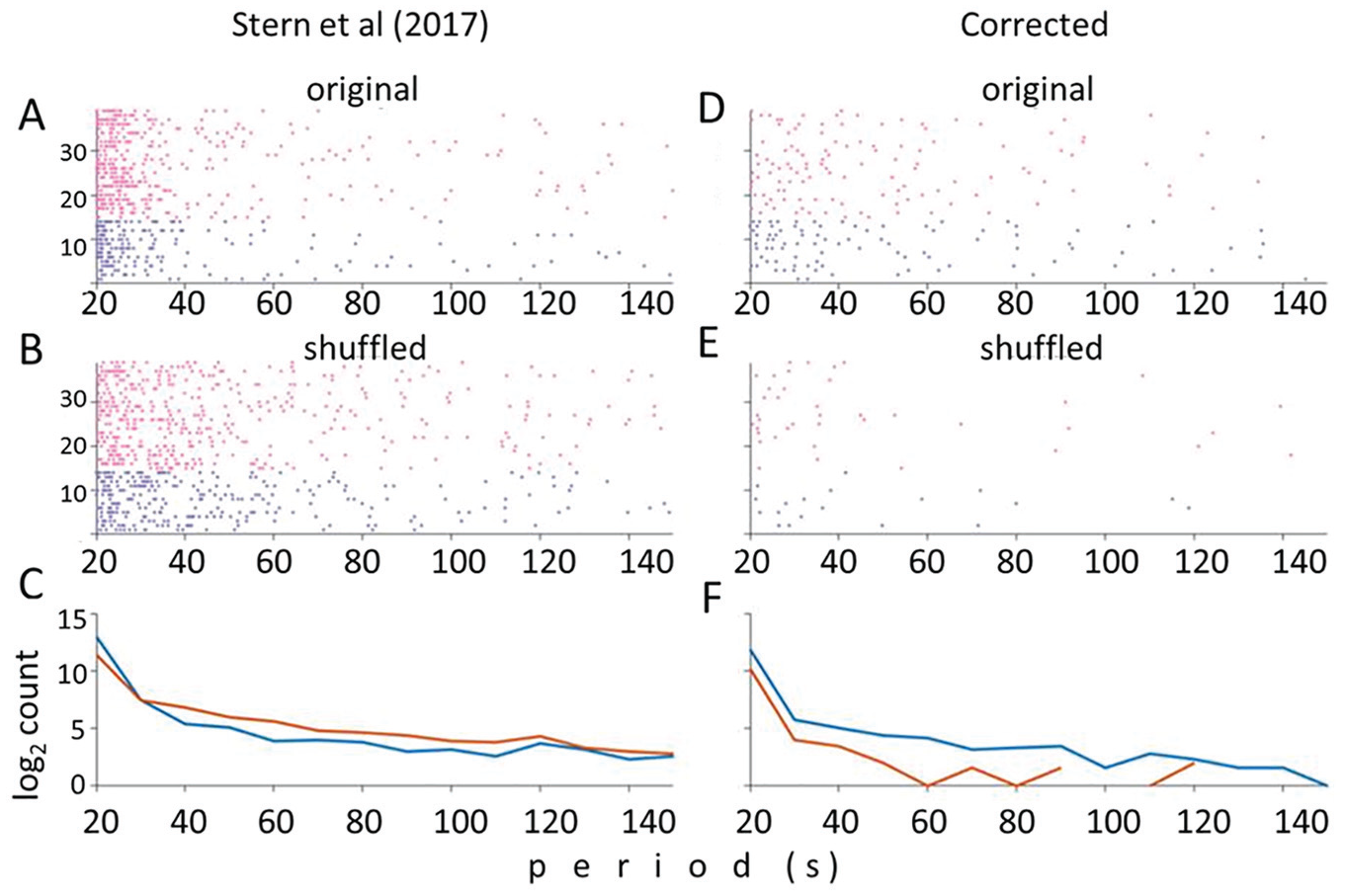
Stern et al. (2017) incorrectly implement the cosinor method. (A-C) Figure redrawn from Stern et al.’s figure S1. Each dot on each horizontal line represents the significant periods by cosinor for a different song: blue the 14 per^L songs and pink the 25 Canton-S songs. (A, B) Results of Stern et al.’s cosinor analysis of the manually annotated data by Kyriacou et al. Similar levels of significance for original (A) and shuffled data (B). (C) Log-scale distribution of significant periods. Note that the shuffled (randomized, brown) distributions are more frequently significant than the original (blue) data. (D-F) Reanalysis of the same data as in (A-C) but correcting Stern et al.’s cosinor coding error so that input period is in radians, not period (see text). (D, E) Many more significant periods are observed in the original data (D) than in the shuffled data (E). (F) Distribution of significant periods. For each period, there are more significant periods in the original than in the randomized data, particularly for longer periods.

We therefore scrutinized their ~2800 lines of code and discovered that their implementation of cosinor was indeed incorrect. Stern et al. (2017) used L-S to generate a series of potential frequencies and then tested each frequency using cosinor. The cosinor implementation used required the tested rhythm to be input as radians (2π/period). However Stern and colleagues had incorrectly imposed the period values into the cosinor algorithm (Figure S1) i.e. fitting corresponding periods from 0.314 to 0.042 s to the ~6 min of annotated song data instead of these values as radians. This will inevitably generate a large number of significant cosinor values for each song, whether the data are randomized or not. In fact, by scanning with such a tiny period range, it would be expected that randomized data, which will show more random fluctuations than real data, would be more likely to reveal significant cycles than real data. In fact, that is exactly what Stern et al. (2017) observed (Fig. 1C).

We corrected the line of code (Suppl. Fig. S1) and reran the cosinor analyses using their platform. Figure 1D-F illustrates that far fewer significant periods are observed in the randomized than in the real data, especially in the longer periods (>50 s), consistent with the results of Kyriacou and Hall (1989). Stern et al.’s (2017) critique of the use of cosinor is therefore simply the result of an error in their implementation of the method. Consequently, there is no valid statistical objection to using cosinor on the results from the studies of K&H and collaborators in the 1980s and early 1990s nor indeed to Kyriacou et al.’s cosinor reanalysis of the manually annotated binned mean IPIs from Stern (2014), in which period-dependent song phenotypes were also observed (Kyriacou et al., 2017). While it is important that the chronobiological community appreciates that cosinor is not flawed as Stern et al. (2017) have claimed, their main focus is on the unbinned data, to which we now turn.

L-S Is Conservative Compared with CLEAN, Cosinor, and Autocorrelation

In their song work of the late 1980s, K&H and colleagues also determined rhythmicity in songs using the CLEAN spectral method, which was developed specifically to analyze unequally spaced data (Roberts et al., 1987). This was a useful method for analyzing mean IPIs, because even though such data were collected every 10 s, there were inevitably gaps in the record when the male did not sing, so these IPI means were unevenly distributed. CLEAN was used to find an initial period for subsequent cosinor curve fitting, but this spectrally derived period was also used as an independent measure of the song cycle (Kyriacou and Hall, 1989; Wheeler et al., 1991). No attempt was made to generate significance levels with CLEAN given the very small number (20-40) of mean IPI data points. We therefore sought to use CLEAN to analyze the unbinned IPIs of songs. However, before embarking on this analysis, we sought to benchmark L-S and CLEAN against 2 other commonly used time-series analyses, autocorrelation and cosinor, using a more conventional circadian/tidal data set from E. pulchra in which locomotor data were collected in equidistant 30-min bins.

Figure 2A shows that L-S and CLEAN produce very similar spectral profiles with similar confidence limits when the 6 days of data, corresponding to ~12 tidal cycles, were robustly rhythmic (as evidenced from the histograms, the time-related period estimates generated from the Morlet wavelet analysis, actograms, autocorrelation, and cosinor). However, when analyzing activity data that were clearly rhythmic (by visual inspection of the histo-/actograms and the Morlet wavelet) but contained more noise or were collected over a shorter time frame, L-S identified nonsignificant peaks in the ~12- or 24-h domain, in sharp contrast to CLEAN, autocorrelation, and cosinor, which found these same cycles to be significant (Fig. 2B-D). Among 258 Eurydice activity records, we observed 91 in which all 4 time-series methods were in agreement but 134 that were significant by CLEAN, cosinor, and autocorrelation but not by L-S. We never observed the opposite, namely, that an activity pattern would be significant by L-S, cosinor, and autocorrelation but not by CLEAN (Suppl. Table S1). Consequently, it appears that L-S is relatively insensitive compared with the other 3 types of time-series analyses, at least for these data. We therefore recomputed L-S confidence limits using 1000 randomizations of each activity record rather than the theoretically derived values. We found that all of the 134 locomotor records that were judged to have significant rhythmicity by all analyses except L-S were now significant using the randomly derived confidence limits (Fig. 2).

Figure 2.

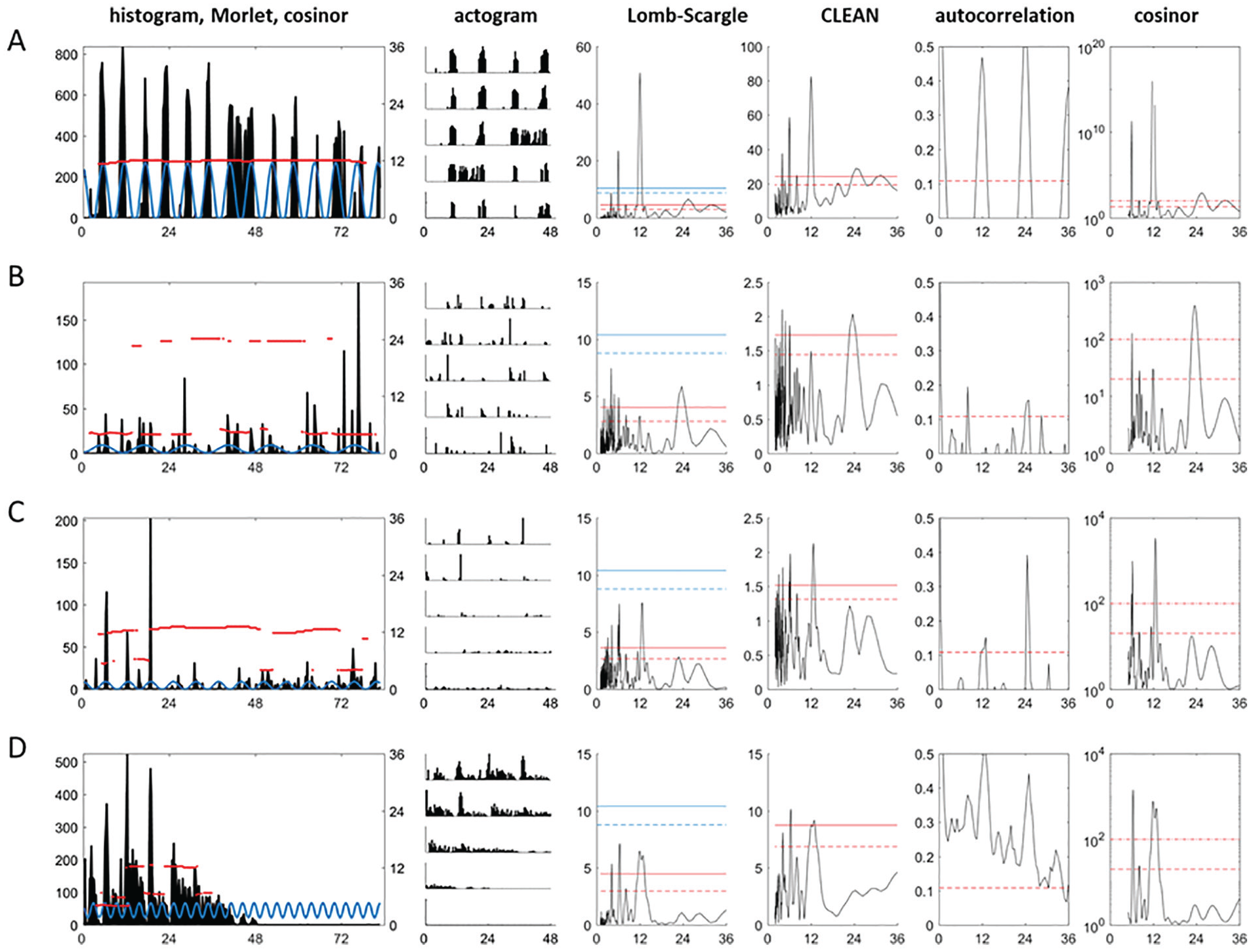
Lomb-Scargle is conservative compared with other time-series methods for locomotor rhythms analyses. (A-D) Analysis of 4 Eurydice pulchra activity patterns. Left-hand column: histogram of locomotor activity for a single animal, with Morlet wavelet shown as red lines corresponding to the right-hand y-axis. The best-fit cosinor is superimposed on the histogram in blue. Second column: double-plotted actogram of the same data. Third column: Lomb-Scargle (L-S) analysis with theoretically derived 95% and 99% confidence limits (blue) and those derived from randomization (red, see text). Fourth column: clean spectral analysis with 95% and 99% confidence limits. Fifth column: autocorrelation with 95% confidence limits; right-hand column. Sixth column: cosinor analysis; the y-axis represents 1/p, and the dotted lines give p values for 95% and 99%. The x-axes are hours. (A) Robust tidal cycles of behavior are significant by each time-series analyses. Confidence limits for L-S based on randomizations are less stringent than those based on theoretical assumptions and match those for CLEAN. (B) Record with noisier data in which Morlet picks out ~6- and ~24-h cycles. These are significant by CLEAN, autocorrelation, and cosinor but not by the standard L-S algorithm using the blue confidence limits. However, the 6- and 24-h cycles are significant by L-S when the confidence limits (red) based on randomizing the time series are used. (C, D) Similar situations to (B) are shown, in which L-S identifies the relevant cycles but assigns them as nonsignificant (arrhythmic) using the theoretically derived confidence limits (blue) in contrast to the other analyses. However, the L-S confidence limits based on randomization (red) render these periods significant.

CLEAN Analysis of Unbinned IPIs Confirms Rhythmicity

Consequently, we reanalyzed the unbinned IPIs for all the per^L and wild-type songs manually annotated by Kyriacou et al. (2017) using L-S with both conventional and randomization-based confidence limits as well as with CLEAN. For CLEAN, we used 2 levels of resolution: the first down to a minimum period of 80 ms (~twice an average IPI), and the second down to a period of 0.4 s. Figure 3 illustrates the song results for L-S using original (blue) and newly-derived (red) confidence limits, alongside those of CLEAN. Song CS14 provides an interesting example, with 3 prominent peaks generated by L-S (Fig. 3A). Stern et al. (2017) scored the peak period as 84.7 s (red arrow), whereas when we ran the same algorithm on the same data, we obtained 65.76 s (blue arrow). Inspection of these 2 peaks from the figure reveals that the 65.76-s peak is slightly higher, but Stern et al. (2017) used an interpolative step in their summarizing code, which generated the longer period of 84.7 s (D. Stern, personal communication). However, both peaks are well short of the theoretically derived confidence limits (blue), so Stern et al. (2017) classified this song as arrhythmic. However, these peaks fall above the L-S confidence limits calculated using randomizations (in red). The CLEAN analysis of CS14 shows again 3 prominent peaks, all above the confidence limits, but the most prominent is at 53.03 s (blue arrow), which was the third highest period found by L-S (Fig. 3A).

Figure 3.

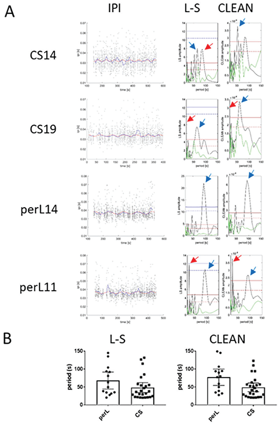
Song rhythms using Lomb-Scargle (L-S) and CLEAN. (A) The left-hand column shows the raw interpulse intervals (IPIs), on which is superimposed the mean IPI based on 10-s bins, and the best sinusoidal fit to the raw data by CLEAN for a selection of songs. The right-hand columns show the L-S periodogram with the corresponding CLEAN spectral analysis. The L-S periodogram has the conventional theoretically derived confidence limits in blue (dotted 95%, unbroken 99%) and those generated from randomly shuffling the data 1000 times in red. The green line represents the analysis of a single random trial. Colored arrows denote peaks (see text). Top row: Wild-type song (CS14) in which Stern et al. (2017; red arrow, 84.75 s) and Kyriacou et al. (2017; blue arrow, 65.8 s) selected different peaks as representing the period of the song cycle using the L-S algorithm. CLEAN distinguishes among the 3 peaks by selecting the third highest (53 s) from the L-S analysis (see text). Row 2: Song CS19. The red arrow denotes a peak period of 19.98 s in the L-S analysis (selected as 20 s by Stern et al., 2017) and the next highest peak at 62.4 s (blue arrow) selected as representing the period of this song by Kyriacou et al. (2017). CLEAN analysis shows the highest peak at 62.3 s (blue arrow); the position of the peak corresponding to 19.98 s (red arrow) is also shown. Row 3: perL14 song showing period at 93.8 s with both spectral analyses. Row 4: Song perL11 with an uncharacteristically short period of 27.6 s (red arrow) but with a highly significant second periodicity at 93.8 s. (B) L-S periods for per^L and Canton-S songs reported by Stern et al. (2017; p = 0.057) and those by CLEAN (this study; p = 0.008).

CS19 (Fig. 3A) provides another example in which Stern et al. (2017) obtained a peak at 19.98 s and rounded up, not unreasonably, to 20 s. The L-S analysis in our hands gave the same peak, but because it was <20 s (position depicted by red arrow), it was ignored, and the highest peak in the >20 s to <150 s range was taken: 62.38 s (blue arrow). The CLEAN analysis also found a peak at <20 s (red arrow) but an even higher peak at 62.34 s (blue arrow), so there is no debate about which is the best period. Song perL14 shows a prominent and significant peak at 93.5 s (blue arrow, Fig. 3A), and song perL11 shows the highest peak at 27 s (red arrow) but another significant peak at 94 s (blue arrow), irrespective of the analyses used. There were 5 per^L songs with L-S (4 with CLEAN) that showed uncharacteristically short-period primary peaks, but all of them had prominent and significant second highest peaks in the per^L range (Suppl. Table S2). For Canton-S, 10 songs had uncharacteristically shorter periods (<35 s), but half of these gave a prominent second highest period in the wild-type range (Suppl. Table S2). The L-S and CLEAN panels of Figure 3A also show the results of a single random trial (green), which reveals that randomized songs generally give nonsignificant or barely significant levels of rhythmicity as expected.

The L-S and CLEAN results for all of the songs can be found in Supplemental Table S2. Using a resolution down to periods of 80 ms, the mean wild-type song period for CLEAN is 49.0 s and for per^L is 76.9 s (p = 0.008, 1-tailed, Fig. 3B, Suppl. Table S2 column F), which can be contrasted with Stern et al.’s (2017) results using L-S (p = 0.057, Fig. 3B, Suppl. Table S2 column C) and our results using L-S, which also show a significant difference between the 2 genotypes (p = 0.028, Suppl. Table S2 column D). Furthermore, if we simply take those CLEAN songs that are significant beyond the 0.05 level, we obtain a very similar statistically significant result (p = 0.018, Suppl. Table S2 column G). At a lower resolution down to 0.4 s, the mean period for wild-type flies is 53.4 s and that for per^L is 79.6 s (p = 0.01, Suppl. Table S2 column I), which is almost identical to the initial results of K&H for these 2 genotypes when the mean IPIs per 10-s bins were analyzed (Kyriacou and Hall, 1980). We conclude that using CLEAN (and L-S with modified confidence limits) on the individual IPIs gives results that are consistent with those based on mean IPIs but with the additional feature that the great majority of the peak periods are statistically significant. Thus, as with the more traditional activity data set described above (Fig. 2), the conventional L-S periodogram would appear to be extremely conservative when analyzing song data.

While the CLEAN analysis focused on periods >20 s to <150 s to match the period range that was scrutinized for 10-s binned data, we also examined the highest peak in the unbinned IPI data for each CLEAN plot between 0.08 and 150 s. Usually, for each song, the highest peak was observed in the very high frequencies (Suppl. Table S2 columns W-Z). Only 1 song for each genotype gave the same peak period as that observed in the 20- to 150-s range (CS2 and perL14). All of the peak periods were significant, and two-thirds were <1 s. There were no significant differences between these peak high frequencies between genotypes by parametric or nonparametric tests (Suppl. Table S2). Similar results were observed with the L-S method as reported previously by Stern (2014) and Kyriacou et al. (2017), but a larger proportion of songs showed peaks <0.4 s with CLEAN. These very short periodicities may represent the interaction between the pattern of IPI within a burst and the interburst interval.

New Song Recordings of Stern et al. Show ~30% Error in the Automated Detection of IPIs

Although the original Stern (2014) CS and per^L data sets have been laboriously corrected using manual annotation (Kyriacou et al., 2017), Stern et al. (2017) have also recorded and analyzed a new set of songs in which they claim an improvement in their automated detection of IPIs from ~50% to ~80%. Their automated analysis using L-S again shows a marginal (p = 0.06) difference between per^L and wild-type song periods, which they dismiss as “noise” because individual songs are not significantly rhythmic. While manual annotation for song rhythm analysis of this new set of songs is out of the question in any reasonable time frame, we did manually examine the first ~100 to 300 IPIs for 30 songs. We observed a remarkable enhancement of the CS song vigor compared with the same strain examined earlier by Stern (2014; Suppl. Fig. S2), which is puzzling and suggests some uncontrolled variation in rearing or maintaining adult flies. We determined that song accuracy varied widely from ~10% to 90% for individual songs (Suppl. Table S3). Most of the errors were omissions, but spurious IPIs accounted for ~12% of the total errors. These were usually of the pulse-skipping type that were reported previously (Kyriacou et al., 2017), when an intervening pulse had been missed, generating a spuriously long IPI (but within the acceptable limits for the upper IPI cutoff) from the 2 flanking pulses. These would have a disproportionate effect on the accuracy of mean IPIs when the IPIs are placed in 10-s bins. The accuracy of the automated method was 73% for the >11,000 IPIs we manually scored (or 65% of the ~9000 IPIs automatically annotated), rather poorer than the figure claimed by Stern et al. and far worse than interobserver manual accuracy, which is 95% to 99% (Kyriacou et al., 2017).

Discussion

There has been considerable debate surrounding the existence of period-modulated rhythmic components in the Drosophila courtship song and the suitability of employing automated, high-throughput recording techniques for their detection (Stern, 2014). Following extensive manual curation of songs that were initially recorded by Stern (2014), these rhythms were detected in both binned and unbinned IPIs despite the experimental shortcomings of the Stern study (Kyriacou et al., 2017). Stern et al. (2017) rejected these conclusions, arguing that (1) the historically employed data-binning approach cannot identify any cycles faster than 20 s; (2) the cosinor method used to analyze IPI cycles in the 1980s generates as many, if not more, false positives in randomized as in real IPI data; and (3) the L-S time-series analysis does not generate significant periodicities for songs based on either binned mean or unbinned IPIs (Stern et al., 2017). While we obviously agree with their first criticism, the insistence that L-S must show significance for each song, even in only 30 to 40 mean IPI data points, is unrealistic (Logan and Rosenberg, 1989). We have demonstrated that Stern et al.’s (2017) objection to cosinor was based on a coding error made by them in implementing the analysis, so it follows that the results from the original studies of Kyriacou, Hall, and colleagues, which were based on cosinor, cannot be so easily disregarded. The correction of Stern et al.’s error will be of some relief to the authors of 1400 papers listed in PubMed that have used this method over the past 5 decades. Cosinor remains a useful method for time-series analysis, particularly for shorter-length data sets such as binned mean IPIs (Cornelissen, 2014).

Stern et al. (2017) therefore shifted their focus to individual IPIs, reporting similar, but less significant, genotype differences as Kyriacou et al. (2017) with the same manually annotated data set using L-S. We have seen that some of these differences depend not on the L-S output but on the way Stern et al. (2017) interpolated the output. However, their most important criticism is their insistence that every song cycle must be significant by L-S or otherwise it simply represents “noise.” Consequently, even though they found a marginal difference in mean song periods between per genotypes, they dismissed it. We therefore compared the L-S method used by Stern et al. (2017) to 3 other time-series analyses using a more conventional binned locomotor activity data set. We observed that L-S detected less than 50% of rhythms that were detected by all 3 other methods: CLEAN, autocorrelation, and cosinor. Clearly, L-S is overly stringent. Indeed, it has been noted previously that L-S underestimates the significance of periodogram peaks in equally spaced data (Frescura et al., 2008). This also holds for unevenly spaced data, partly because realistic theoretical confidence limits are extremely difficult to calculate and so more pragmatic randomization methods are preferred (Frescura et al., 2008).

These limitations of L-S were confirmed by our analysis of the circadian/tidal data set, which underlined the insensitivity of L-S compared with CLEAN, autocorrelation, cosinor, Morlet wavelet, or even visual inspection of histograms/actograms. When we recalculated confidence limits based on 1000 randomizations of each locomotor record, we observed that L-S now gave almost identical results to the other methods in terms of the significance of individual locomotor records. We then applied this modified L-S to the irregularly spaced song data and compared with CLEAN. With CLEAN, we observed statistically significant cycles in individual songs and significant genotypic differences between per^L and wild type, irrespective of the resolution used and with mean period lengths almost identical to K&H’s original findings based on mean binned IPIs (Kyriacou and Hall, 1980). In contrast to the conventional L-S used by Stern et al. (2017), most songs were also significantly rhythmic, with the modified L-S confidence limits generating similar genotypic differences as CLEAN. Even though L-S has been reported to be less robust than other time-series analyses when the data contain a large proportion of gaps such as song records (Munteanu et al., 2016), the new confidence limits appear to compensate for this problem.

Noisy data that are unevenly spaced create problems for time-series analyses, irrespective of the method employed. Both L-S and CLEAN have been developed to solve these problems. L-S is a “dirty” spectrum, whereas CLEAN was specifically designed to remove noise associated with the sampling frequency associated with unequally spaced data (Roberts et al., 1987). The consensus from several discourses on these methods is that data collected in this manner should be analyzed with a variety of methods (Hocke and Kampfer, 2009; Pardo-Iguzquiza and Rodriguez-Tovar, 2015; Schimmel, 2001). We have used 2 different spectral methods for unbinned IPIs (L-S and CLEAN) and 4 methods for binned mean IPIs (CLEAN, L-S, cosinor, autocorrelation; Kyriacou et al., 2017), whereas Stern and colleagues (2017) preferred to use only 1 overly stringent method, L-S, for both unbinned and very short-series binned data.

Finally, a manual annotation of short stretches of the new songs that Stern et al. (2017) recorded and that they claim ~80% accuracy compared with ~50% from Stern (2014) revealed an accuracy of ~70%, which, while a significant improvement, still leaves a ~30% error rate. These accuracy levels are still far lower than the interobserver accuracy from manual annotation, which reaches 99% and is not less than 95% (Kyriacou et al., 2017). To counter this obvious objection to automation, and to the 50% error rate detected in Stern’s (2014) original data, Stern et al. (2017) performed a series of simulations and power calculations in which they generated sinusoidal IPIs, manipulated the signal in various ways, and concluded that if there is a rhythm in individual IPIs, L-S will detect it (Stern et al., 2017). As the input signal is sinusoidal (or sawtooth), we are not surprised that the algorithm detects the sinusoid. However, it is telling that the real song data from Stern (2014) that was manually annotated and is as close as possible to 100% accuracy fails the conventional L-S significance levels yet passes those for CLEAN and the modified L-S. This suggests that simulated sinusoidal IPI data that are manipulated in these ways do not provide a realistic model of the song rhythms generated by the fly.

Nevertheless, Stern and colleagues (2017) have illustrated the enormous variability of IPI within a single song, which has not been appreciated before. This is in stark contrast to the early work on fly songs, in which it was implied that the IPIs are invariant and species specific, generating an unambiguous species signature (Ewing and Bennett-Clark, 1968). Given the variation in IPIs within a single song (from 15-100 ms), it does suggest that the female may average the signal to make any sense of it. If so, then the male may average his IPIs in a manner that may stimulate a female’s preferred range of IPIs, and a rhythmically varying mean IPI may provide a strategy for stimulating a greater number of females. In fact, playback experiments reveal that species-specific rhythmically varying IPIs optimally stimulate the female for mating (Kyriacou and Hall, 1982, 1986; Ritchie et al., 1999). As the variation in individual IPIs is high (see Fig. 3), the females must be averaging IPI over time frames of several seconds in order to respond preferentially to the different species-specific cycles (Kyriacou and Hall, 1982, 1986; Ritchie et al., 1999).

To conclude, although Stern and collaborators (2017) cannot replicate the song rhythm work, their analyses of the manually corrected data as well as of their uncorrected data from their new songs come tantalizingly close to revealing the wild-type/per^L differences, which is encouraging. The 3 main reasons they fail to replicate the K&H results are the following. (1) Their automated data-capture methods have a 30% to 50% error rate, which is not helpful (Stern, 2014; Stern et al., 2017). We appreciate that automation is the only way that high-throughput song analysis can be performed efficiently and would not wish to stand in the way of the considerable progress that has been achieved by Stern and colleagues on this front. However, our manual/automation comparisons do underline the fact that for short time frames of 10 s or less (the time of a song bin in K&H studies), automation may add considerable uncertainty to the song phenotype under study, mainly because of omission. (2) Stern et al. (2017) incorrectly implemented the cosinor method on which the original studies of K&H and collaborators were based. When cosinor was used appropriately on binned mean IPIs, period-dependent cycles were observed in Stern’s data (Kyriacou et al., 2017). (3) When Stern et al. (2017) extended the analysis to the manually annotated unbinned IPIs, they used only a single time-series method, L-S, which we show here is extremely conservative both for more traditional equidistant data sets and for the irregularly spaced unbinned IPI data. When L-S confidence limits are recalculated using randomizations, the results from the L-S algorithm are consistent with those from other methods for locomotor and song data. Both the modified L-S and the CLEAN methods generate significance in the unbinned IPIs of individual songs and produce period-specific phenotypes that match almost exactly those first identified in binned IPI means by K&H (Kyriacou and Hall, 1980).

Supplemental Material

Copy_of_TableS3newrevison – Supplemental material for A Computational Error and Restricted Use of Time-series Analyses Underlie the Failure to Replicate period-Dependent Song Rhythms in Drosophila

Supplemental material, Copy_of_TableS3newrevison for A Computational Error and Restricted Use of Time-series Analyses Underlie the Failure to Replicate period-Dependent Song Rhythms in Drosophila by Charalambos P. Kyriacou, Harold B. Dowse, Lin Zhang and Edward W. Green in Journal of Biological Rhythms

Supplemental Material

FinalSupplementary_Figures_and_References – Supplemental material for A Computational Error and Restricted Use of Time-series Analyses Underlie the Failure to Replicate period-Dependent Song Rhythms in Drosophila

Supplemental material, FinalSupplementary_Figures_and_References for A Computational Error and Restricted Use of Time-series Analyses Underlie the Failure to Replicate period-Dependent Song Rhythms in Drosophila by Charalambos P. Kyriacou, Harold B. Dowse, Lin Zhang and Edward W. Green in Journal of Biological Rhythms

Supplemental Material

TableS2revisedNov14 – Supplemental material for A Computational Error and Restricted Use of Time-series Analyses Underlie the Failure to Replicate period-Dependent Song Rhythms in Drosophila

Supplemental material, TableS2revisedNov14 for A Computational Error and Restricted Use of Time-series Analyses Underlie the Failure to Replicate period-Dependent Song Rhythms in Drosophila by Charalambos P. Kyriacou, Harold B. Dowse, Lin Zhang and Edward W. Green in Journal of Biological Rhythms

Supplemental Material

Table_S1 – Supplemental material for A Computational Error and Restricted Use of Time-series Analyses Underlie the Failure to Replicate period-Dependent Song Rhythms in Drosophila

Supplemental material, Table_S1 for A Computational Error and Restricted Use of Time-series Analyses Underlie the Failure to Replicate period-Dependent Song Rhythms in Drosophila by Charalambos P. Kyriacou, Harold B. Dowse, Lin Zhang and Edward W. Green in Journal of Biological Rhythms