An Exploration of the Temporal Dynamics of Circadian Resetting Responses to Short- and Long-Duration Light Exposures: Cross-Species Consistencies and Differences

Abstract

Light is the most effective environmental stimulus for shifting the mammalian circadian pacemaker. Numerous studies have been conducted across multiple species to delineate wavelength, intensity, duration, and timing contributions to the response of the circadian pacemaker to light. Recent studies have revealed a surprising sensitivity of the human circadian pacemaker to short pulses of light. Such responses have challenged photon counting–based theories of the temporal dynamics of the mammalian circadian system to both short- and long-duration light stimuli. Here, we collate published light exposure data from multiple species, including gerbil, hamster, mouse, and human, to investigate these temporal dynamics and explore how the circadian system integrates light information at both short- and long-duration time scales to produce phase shifts. Based on our investigation of these data sets, we propose 3 new interpretations: (1) intensity and duration are independent factors of total phase shift magnitude, (2) the possibility of a linear/log temporal function of light duration that is universal for all intensities for durations less than approximately 12 min, and (3) a potential universal minimum light duration of ~0.7 sec that describes a “dead zone” of light stimulus. We show that these properties appear to be consistent across mammalian species. These interpretations, if confirmed by further experiments, have important practical implications in terms of understanding the underlying physiology and for the design of lighting regimens to reset the mammalian circadian pacemaker.

Introduction

The phase of the mammalian circadian pacemaker can be shifted by environmental light. The size of the phase shift depends on the wavelength, intensity, duration, and timing of the light stimulus (Nelson and Takahashi, 1991; Czeisler, 1995; Zeitzer et al., 2000; Khalsa et al., 2003; Lockley et al., 2003; Comas et al., 2006; Czeisler and Gooley, 2007; Dkhissi-Benyahya et al., 2007; Gooley et al., 2010; Chang et al., 2012; St Hilaire et al., 2012; Rüger et al., 2013; Rahman et al., 2017). These responses have been extensively studied in both nocturnal and diurnal mammals, including humans. Understanding these responses is crucial for basic science and translation to applications. We focus here on light intensity and duration factors that influence these phase shifts by analyzing results from multiple mammalian species.

The circadian phase-resetting system has often been assumed to act like a “photon counter” (Nelson and Takahashi, 1991; Lall et al., 2010; Brown, 2016) that predicts linear increasing phase shift with increasing photons (from either intensity or duration). This assumption, however, is not consistent with observations in multiple species (Kronauer et al., 1999; Vidal and Morin, 2007; Zeitzer et al., 2011; Najjar and Zeitzer, 2016). For example, we recently published 2 articles (Chang et al., 2012; Rahman et al., 2017) summarizing the temporal dynamics of human delay phase shifts achieved for a range of light exposure durations, T, extending from 15 sec to 6.5 h, that show that the response is not linear, as would be expected for a system that counts photons. These results prompted us to analyze data to assess the temporal dynamics of photic resetting responses from multiple species.

The particular data sets on which we focus in the upcoming sections were chosen based on 2 factors: (1) responses were elicited by at least 3 different light stimulus durations and (2) data could be extracted directly from the publications (i.e., from figures or tables). Four data sets across 4 different mammalian species met our criteria. We begin our discussion with delay phase shifting in humans and c-fos induction in gerbils in response to different light durations to introduce our mathematical formulation for short-duration light stimuli. We then discuss the interaction between light intensity and duration in golden hamsters and phase shifting in mice before introducing a formal model.

Human Phase-Resetting Responses to Light: Differences Between Short- and Long-Duration Exposures

Our human phase-delay resetting data are summarized in Table 1 (Gronfier et al., 2004; Chang et al., 2012; Rahman et al., 2017). Targeted corneal illumination for all stimulus durations was ~9500 lux (>8 × 10⁶ µW/cm²) generated using ceiling-mounted 4100K fluorescent lamps. The first robust finding from this data set (Table 1; Figure. 1) is the monotonic decline of the yield or resetting rate ( $\frac{\mathit{y}}{\mathit{T}}$ , minutes of phase-delay shift per minute of light exposure) with increasing stimulus duration (T; note that T refers to stimulus duration, not time). Simply interpreted, for any light stimulus duration, it is the early photons that have the disproportionately largest effect. As the stimulus proceeds (i.e., longer duration), later photons have progressively less effect. We will now quantify this effect.

Table 1.

Phase-delay shifts and shift rate of the human duration response curve.

T: Duration of Light Exposure (min)	Y: Delay Shift (Median ± SD, min)	$\frac{\mathit{y}}{\mathit{T}}$ : Resetting Rate (i.e., Minute of Phase Shift per Minute of Light Exposure)
0.25	34.8 ± 47.2	139.2
2.00	45.4 ± 28.4	22.7
12.00	74.2 ± 35.2	6.2
60.00	102.6 ± 35.6	1.7
150.00	120.6 ± 37.2	0.8
240.00	134.5 ± 46.8	0.6
390.00	183.0 ± 27.0	0.5

Figure 1.

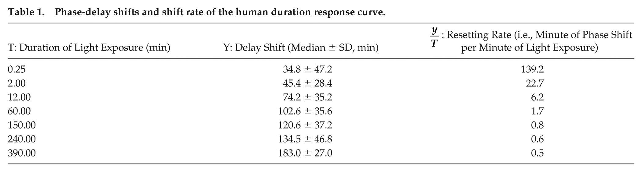
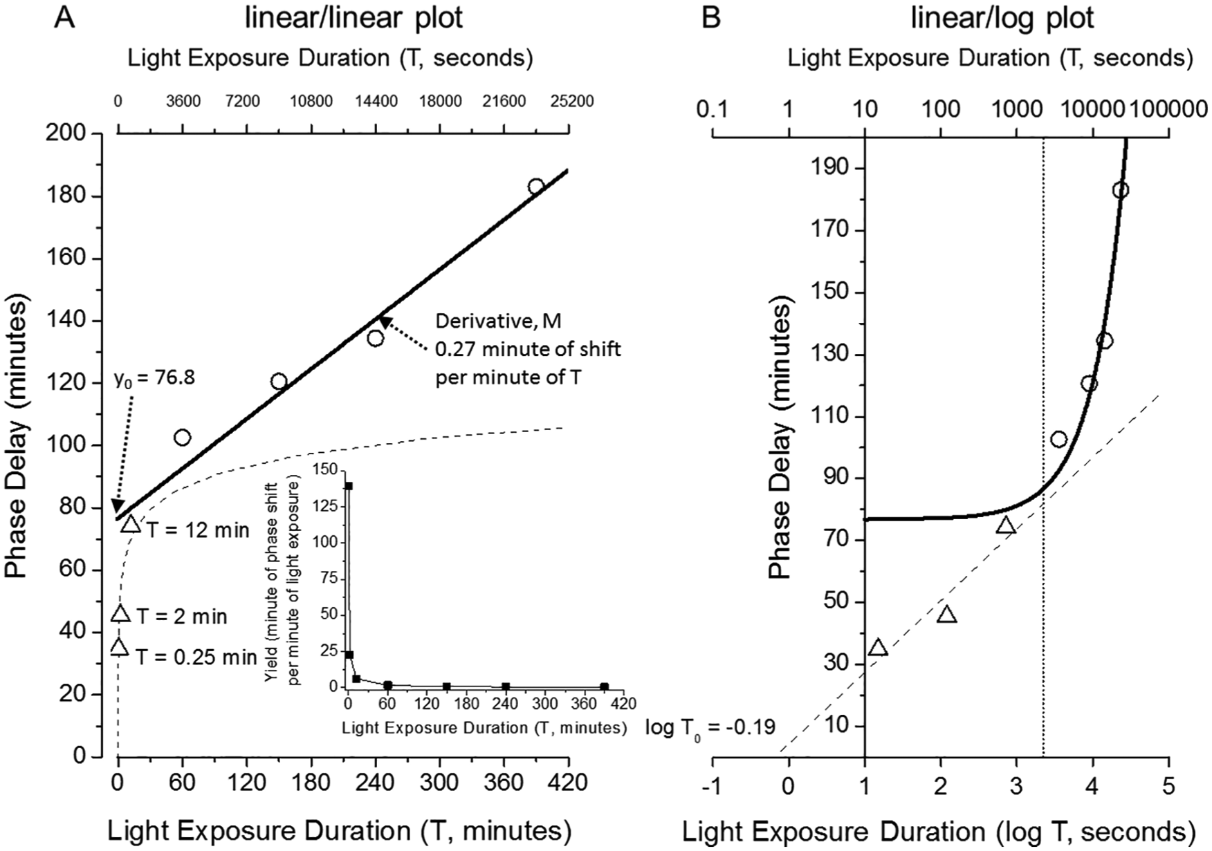
(A) The human duration response curve spanning very short (0.25 min) to long (390 min) light exposure durations reveals a nonlinear relationship with an approximately linear response for T > 60 min (omitting T = 60 min from the fit; circles, solid line) and approximately log response for T < 60 min (triangles, dashed line). The inset shows the yield (resetting rate, $\frac{\mathit{y}}{\mathit{T}}$ ) as a function of light exposure duration. (B) The same phase-delay shifts plotted on a log scale for T > 3600 sec (i.e., omitting T = 3600 seconds from the fit; circles, solid line) and T < 3600 sec (triangles, dashed line). The vertical line indicates the approximate light exposure duration at which a transition between asymptotic states occurs.

When these data are plotted (Figure. 1A), the rate at which the average phase shift is increasing with longer stimulus durations (T, in minutes) appears different for the 3 shortest duration stimuli (T ≤ 12 min ) as compared with the 3 longest duration stimuli (T ≥ 150 min), with the 3 longest duration stimuli appearing to be linear. We fit a linear regression through the resetting responses from the 3 longest duration stimuli, which results in an intercept (y₀) of 76.75 min and a slope of the resetting rate M = $\frac{\mathit{d}\mathit{y}}{\mathit{d}\mathit{T}}$ of 0.27 min of phase shift per minute of light exposure (adjusted R² = 0.95). The response elicited by T = 60 min to bright light is not included in the fit applied to either the short- or long-duration stimuli; in our description below of the leaky integrator model, we will discuss why T = 60 min (3600 sec) is not included in these first calculations.

To explore the phase-resetting responses from the 3 shortest-duration stimuli (T ≤ 12 min), we choose a strongly nonlinear transformation of T: x = log T, where the original unit of minutes has been converted to seconds (Figure. 1B). The relationship between phase shift and x = log T for the 3 longest-duration stimuli now appears exponential, and the relationship between phase shift and x = log T for the 3 shortest-duration stimuli appears to be linear (Figure. 1B). This linear fit is expressed mathematically as

$$y=m(x-x_0)$$

(1)

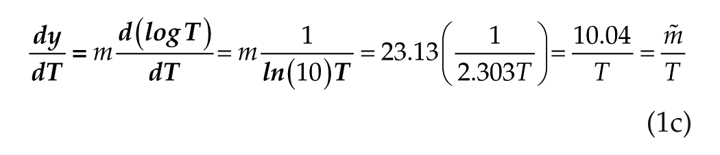
where m = $\frac{\mathit{d}\mathit{y}}{\mathit{d}\mathit{l}\mathit{o}\mathit{g}\mathit{T}}$ . Note that we use m for the short-T relationship and M for the long-T relationship.

We find m = 23.13 min and $x_0$ = −0.19. This value for $x_0$ translates into a stimulus duration of $T_0=10^{x_0}$ = 0.65 sec (n = 3, adjusted R² of 0.95), which represents the response onset of the system. We now write the short T (light duration ≤12 min) relationship in its primary form:

$$\mathrm{y}=\mathrm{m}\left(\log \mathrm{T}-{\log \mathrm{T}}_0\right)$$

(1a)

or equivalently,

$$\mathrm{y}=\mathrm{m}\log (\frac{T}{T_0})$$

(1b)

(Note: we are using log [base 10] rather than ln [base e] here since the data are in log units. We convert to ln later for ease of calculations.) This relationship embodies only 2 parameters, m and T₀. It has an elegant simplicity, and we refer to it as the linear/log function. Later in this article, we will analyze data from several mammalian species (gerbil, hamster, and mouse) that suggest their responses to short-duration light stimuli display this same linear/log functionality.

In Figure 1B, we now have 2 cases: linear/log for the 3 shortest-duration stimuli and linear/linear for the 3 longest-duration stimuli. It is immediately apparent from Figure 1B that the 2 cases do not intersect, although they come close. We undertake to calculate the stimulus duration T^* at the closest approach. We observe that at the closest approach, the 2 curves must show the same $\frac{\mathit{d}\mathit{y}}{\mathit{d}\mathit{x}}$ and therefore the same $\frac{\mathit{d}\mathit{y}}{\mathit{d}\mathit{T}}$ . For long T, $\frac{\mathit{d}\mathit{y}}{\mathit{d}\mathit{T}}$ = M. For the 3 shortest-duration stimuli, we have from equation 1b that

$$\frac{\mathit{d}\mathit{y}}{\mathit{d}\mathit{T}}=m\frac{\mathit{d}\left(\mathit{l}\mathit{o}\mathit{g}\mathit{T}\right)}{\mathit{d}\mathit{T}}=m\frac{1}{\mathit{l}\mathit{n}\left(10\right)\mathit{T}}=23.13\left(\frac{1}{2.303T}\right)=\frac{10.04}{T}=\frac{\tilde{m}}{T}$$

(1c)

where ln 10 = 2.303 when we convert from log to ln to analyze the derivative. Because, in this equation, T occurs in the denominators of both $\frac{\mathit{d}\mathit{y}}{\mathit{d}\mathit{T}}$ and $\frac{10.04}{T}$ , we are free to assign to T whatever units we choose; here, we choose minutes. Equating the derivatives M = 0.27 = $\frac{10.04}{T}$ (where 0.27 is derived from long-T stimuli and 10.04 is derived from short-T stimuli) gives T^* = $\frac{10.04}{0.27}$ = 37.19 min and ln T^* = 3.62.

At this point, we address several fundamental concepts. In the immediately preceding paragraph, we treated the linear/log and linear/linear cases as mathematical equals. One goal of this article is to show how the linear/log function, which is presented formally below in equation 3, is encountered across mammalian species; how it works for both advance and delay phase shifts; how it functions independently of the intensity of the light stimulus; and how time dependence is embodied in the single parameter T₀, which shows remarkable consistency across species. In contrast, the linear/linear function, which we discuss below in equation 11, is probably relevant solely to the delay region of induced phase shifting. This is because if the stimulus can produce a moderately strong continuous phase-delay shift, it can significantly counteract the intrinsic progression of the circadian pacemaker (due to the longer than 24-h intrinsic period), thus allowing the stimulus yet more time to persist in the peak delay region. In contrast, a stimulus that can produce a moderately strong continuous phase advance shift would enhance the intrinsic progression, moving phase away from the peak advance region.

We shall elaborate below on the richness of the linear/log function, but first we must comment on the paucity of data from which this function was extracted. The entire data set contains only 3 phase-shift values found for light durations from T = 15 sec (0.25 min) to T = 720 sec (12 min), representing a range of 1.7 log units, and 3 phase shift values from T = 150 to 390 min. The parameter T₀ = 0.65 sec (calculated above) is 1.4 log units shorter than the shortest stimulus duration for which we have data. To support our finding of the linear/log function, therefore, we digress in the next section to examine the stimulus response in gerbils.

Light Pulse Duration Studies Using C-Fos Induction in the Gerbil Suprachiasmatic Nucleus

In casting about for other reports against which to test our proposed linear/log representation of overt circadian response to brief light pulses (e.g., T < 1000 sec), we discovered the remarkable study by Dkhissi-Benyahya and colleagues (2000) that used c-fos induction to evaluate circadian phase shifts to light in gerbils. In Dkhissi-Benyahya et al., wild-caught gerbils (a diurnal species) previously acclimated to a 12:12 light:dark cycle were placed in constant darkness on test day and stimulated with 500-nm monochromatic light pulses (3.8 × 10⁻¹ µW/cm²) at CT16 (i.e., 16 h after normal lights-on and 4 h into the subjective night); this light stimulus is expected to produce a phase delay. A range of stimulus durations from T = 3 sec to T = 2850 sec was tested (n = 4 per stimulus). Following the light stimulus, animals were returned to total darkness. One hour after the start of light exposure, gerbils were sacrificed, and the optical density of c-fos–labeled cells in suprachiasmatic nucleus (SCN) sections was determined relative to background.

This experiment had at least 2 clear objectives. The first was to quantify, in terms of optical density of c-fos-labeled cells, the saturation of response with increasing light intensity (in units of photons/cm²/sec). Figure 1A of the Dkhissi-Benyahya et al. (2000) study, in which they report 3.74 × 10¹² photons/cm²/sec as the half-saturation intensity for a stimulus duration of 15 min, shows success with this objective. We compare this to the 1.4 × 10¹¹ photons/cm²/sec as the half-saturation intensity for a stimulus duration of 5 min in the most extensive saturation study completed by Nelson and Takahashi (1991) in the golden hamster; we discuss this study further below. The similarity of the 2 results and the underlying physiological relationship supports our hypothesis that the optical density of c-fos induction may be comparable with phase shifts in our investigation of the linear/log function; this relationship is also documented in Trávnícková et al. (1996) and Muscat and Morin (2005).

A second objective of the Dkhissi-Benyahya et al. (2000) experiment was to demonstrate that optical density of c-fos induction saturates with increasing stimulus duration from 3 to 2850 sec (their figure 1B). To convert their optical density data to values that we might compare to human phase-shift data, we measured numerical values for these densities (D) from a photo enlargement of their figure 1B and then subtracted the reference density (dark control, D₀). The values on the x-axis have been converted to log T in our Table 2 and Figure 2A.

Table 2.

c-fos induction in the suprachiasmatic nucleus in response to a range of stimulus durations.

T (sec)	x = log T	y = D − D0	Scaled y
3	0.48	7,450	19.67
9	0.95	6,020	15.89
15	1.18	12,400	32.74
28	1.45	14,930	39.42
90	1.95	18,810	49.66
285	2.46	22,910	80.48
900	2.95	21,040	55.55
2,850	3.46	34,030	89.84

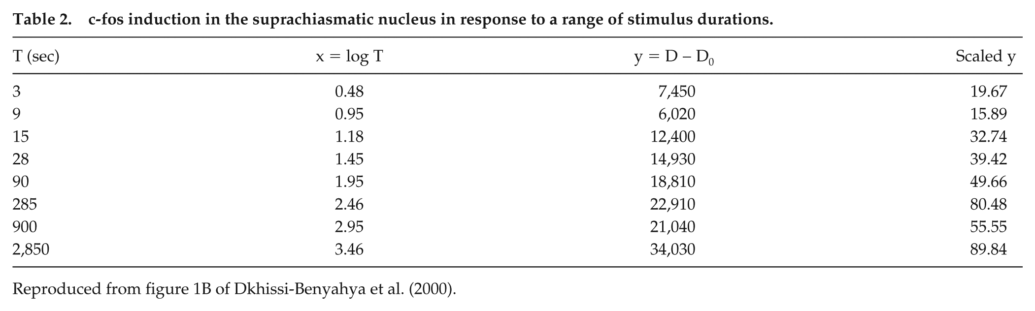
Reproduced from figure 1B of Dkhissi-Benyahya et al. (2000).

Figure 2.

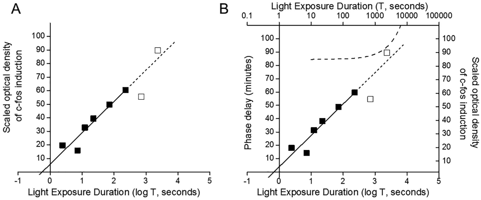
(A) Optical density of c-fos induction in the suprachiasmatic nucleus in response to a range of stimulus durations (log T, sec), as originally reported in Dkhissi-Benyahya et al. (2000), was scaled by the optical density in the dark control and divided by a factor of 1000 for ease of display. Data over the range of T = 3 sec to T = 285 sec (filled squares) were fit by a linear regression (solid line) with an extrapolation to T = 2850 sec (dashed line) for data for T > 300 sec (open squares). (B) Optical density of c-fos induction in gerbils (square symbols and solid line fit with dashed-line extrapolation to T = 2850 sec) and the linear/linear fit (dashed line) to long-T phase-delay shifts in humans (from Fig. 1B) are plotted on the same graph for comparison.

All 8 points of the gerbil data are plotted in Figure 2A. The first 6 points span the T-range of the data from Nelson and Takahashi (1991), which we discuss in further detail below. In Figure 2A, we also show the linear/log fit to these first 6 points as a solid line with extrapolation to the 2 points at longer T as a dashed line. The parameters of this linear/log fit are as follows: intercept T₀ = 0.69 sec, slope m = 8.76= $\frac{dy}{d\log T}$ , adjusted R² = 0.91. We compare these data with the human data, for which the linear/log parameters are T₀ = 0.65 sec, m = $\frac{dy}{d\log T}$ = 23.13, adjusted R² = 0.91. First, we regard the close match of the T₀ values for human and gerbil (0.65 vs. 0.69, respectively) to be remarkable. We propose rescaling the gerbil data by the multiplier $\frac{m_{human}}{m_{gerbil}}=\frac{23.13}{8.76}=2.64$ and then dividing this product by a factor of 1000, to bring the c-fos induction data to the same scale as human phase-shift data. These rescaled values are included in Table 2.

We next transfer the linear/linear function for humans from Figure 1B to Figure 2B. To this figure, we add the 8 scaled data points from gerbil. The slope of the first 6 gerbil data points (i.e., in the short T domain) match the slope of the human data (dashed line in Figure 1B) exactly, which is expected given our choice of scaling factor. From Figure 2, we observe that the final T in the gerbil data lies beyond T^* = 37.19 min (2230 sec), which represents the transition point to the linear/linear process in the human data. It is remarkable how close the data point at the longest T in the gerbil data comes to the human long-T function. The data point at the second longest T in the gerbil data (T = 900 sec) is perplexing, however. As shown in Figure 2B, not only does this data point lie 15 y-units below the linear/log fit, it also lies approximately 5 y-units below the data at T = 285 sec, which represents a difference in stimulus duration of only 10.25 min (615 sec).

In summary, the central 4 points of the gerbil data (from T = 15 to T = 285 sec) fit our proposed linear/log process extremely well, and the extension to the shortest 2 data points (T = 3 and 9 sec) is also satisfactory. The data at T = 2850 sec, which was the longest possible stimulus duration within the experimental framework, suggests a transition out of the linear/log process, not unlike that observed in the human data.

Implications of the Linear/Log Function

We have now presented 2 mammalian species for which a response measure (phase-delay shifts for humans and generation of c-fos–labeled cells in the SCN for gerbils) shows an apparent linear/log process (an increase in phase shift proportional to the logarithm of the duration of light stimulus) of photic stimulation for a relatively short stimulus durations. The mathematics of the linear/log function were discussed in equation 1 and in the 2 equivalent forms introduced in equations 1a and 1b. To understand the process that occurs at short duration stimuli, we use the concept of yield, $\frac{dy}{dT}$ : the ratio of incremental output to incremental “drive,” that is, the incremental phase shift per incremental light stimulus duration. In equation 1c, we noted that yield = $\frac{dy}{dT}$ = $\frac{\tilde{m}}{T}$ . The interesting features of this result are, first, that yield is not simply declining but being driven down inversely with increasing T and, second, that the relevant time is measured from light onset (T = 0) rather than the response onset, T₀.

In their introduction, Dkhissi-Benyahya and colleagues (2000) stated, “A single short pulse of light (<1 sec) fails to induce a phase shift of locomotor activity, which generally requires longer durations of light exposure.” No reference to this statement is given, but by projecting the linear/log function back to T₀, which is <1 sec in both our human phase-delay data and their gerbil c-fos induction data, we can quantify the limit hinted at in their statement. At the same time, this backward projection reveals a remarkable finding: yield attains its maximum value, $\frac{\tilde{m}}{T_0}$ at T₀ since T₀ is the shortest possible response onset time. Therefore, T₀ has 2 possible interpretations: (1) the stimulus duration at which response can first be detected and/or (2) the shortest single stimulus duration for which the response can be sustained.

We note that in equation 1, y could increase without limit (i.e., never saturate). Human phase-delay shift data show, however, that this linear/log relationship morphs into a linear/linear relationship (Figure. 1A) beginning at approximately T = 1000 sec (log T = 3.00 log sec) and is complete by approximately T = 7000 sec (log T = 3.85 log sec). The process that ultimately limits the circadian phase-delay shift is complicated, which we approach in our discussion of the leaky integrator model later in this paper.

A Trove of Hamster Responses to Brief Light Pulses: Separating Brightness and Duration

Throughout our analysis of the effect of stimulus duration so far, the character of the stimulus (e.g., the intensity or the spectrum) was held constant. The coefficient, $\tilde{m}$ , however, would also be expected to be an increasing (and probably saturating) function of brightness.

We now turn to the remarkable and comprehensive article of Nelson and Takahashi (1991) that includes both advance and delay shifts in the nocturnal golden hamster over a stimulus duration (T) range of several log units as well as an intensity (I) range of several log units. From this plethora of riches, we have selected the results shown in their figures 4 and 5, which are in the phase-advance region of the phase-response curve (PRC). The timing of these pulses (CT19) is in a regime in which the response is large but the decline of the response rate with time is also strong (e.g., see the PRC in their figure 2). The data range that is useful to us for the purposes of understanding the short T regime is T ≤300 sec (5 min). Intensity, I, is reported in terms of photon flux density (photons per cm² per second). We use labels of E11 to E14 to designate 10¹¹ to 10¹⁴ photons per cm² per second. Light pulses in this study were generated from a tungsten-halogen lamp (λ_max = 503 nm).

Nelson and Takahashi (1991) arranged the experiment by selecting duration, T, on a coarse grid and varying light intensity, I, in small steps. The durations were arranged in a decimal series (T = 3, 30, and 300 sec). Raw phase-shift data (phase advances, in minutes) for T = 300 sec were extensively sampled (i.e., multiple animals at more than 12 intensity values), whereas at T = 30 sec, only 4 intensity values were sampled. Similarly, at T = 3 sec, only 6 intensity values were sampled and only at 4 intensity values were multiple animals studied. In Figure 3, we show these ranges (E11-E14).

Figure 3.

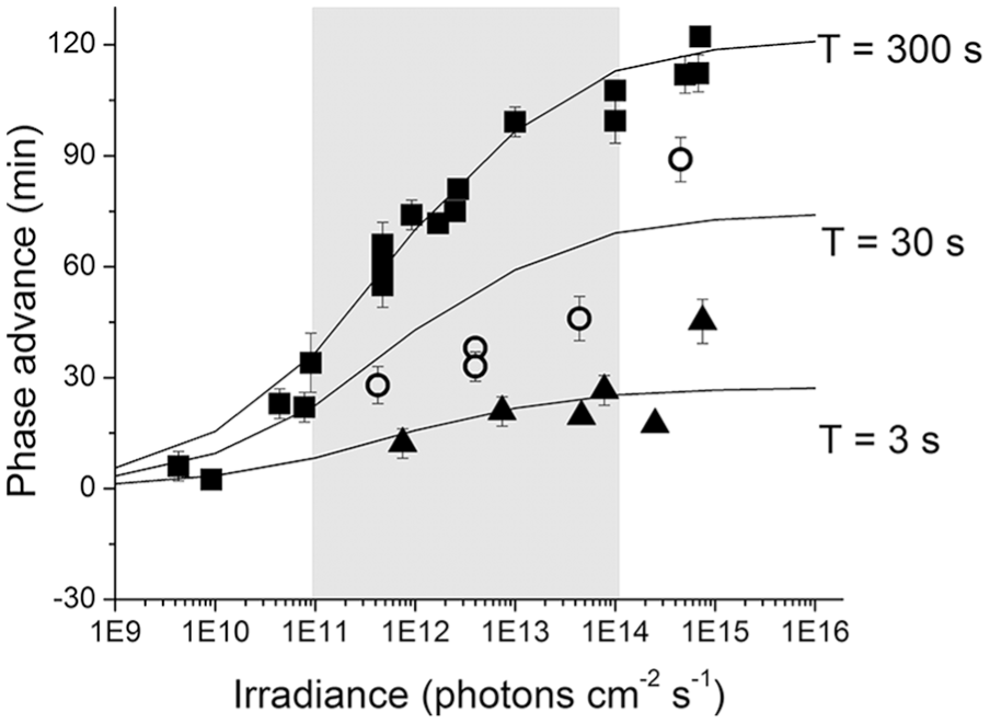
A comparison of the raw golden hamster phase advance data (mean ± SEM) as originally reported in Nelson and Takahashi (1991; filled triangles, T = 3 sec; open circles, T = 30 sec; filled squares, T = 300 sec) with estimates of our linear/log model (solid lines, model as reported in equation 3). The light gray bar denotes the irradiance range over which our analysis was focused.

Nelson and Takahashi (1991) fit a 4-parameter Naka-Rushton function to each T:

$$y=\frac{y_{max}-y_{min}}{1+{\frac{\sigma }{I}}^n}+y_{min}$$

(2)

where y is the phase-shift response in minutes, σ is the stimulus required to achieve the half-maximal response, and n is the steepness or slope of the function. y_max represents the asymptotic fit as I → ∞ and y_min represents the asymptotic fit as I → 0. For T = 300 sec, the raw data are plentiful, and the asymptotes were first fixed by the data (see the figure 4 caption in Nelson and Takahashi for details). For I → 0, the calculated asymptotic shift was −6 min, which Nelson and Takahashi indicated was “not significantly different from zero,” whereas for I → ∞, the calculated asymptotic shift was 114 min, which was then used as the maximum possible phase shift for stimulus durations of 3, 30, and 300 sec. Note that (1) the alteration of y₀ from −6 min to 0 min for T = 300 sec gives us a criterion of ±6 min from which we can assess the relative range for subsequent data manipulation, and (2) contrary to their assumption, a constant maximum shift of y = 114 min that was calculated for T = 300 sec may not be appropriate for T = 3 or 30 sec; they do not have data at higher intensities for these durations to confirm whether a similar constant maximum shift is achieved.

Figure 4.

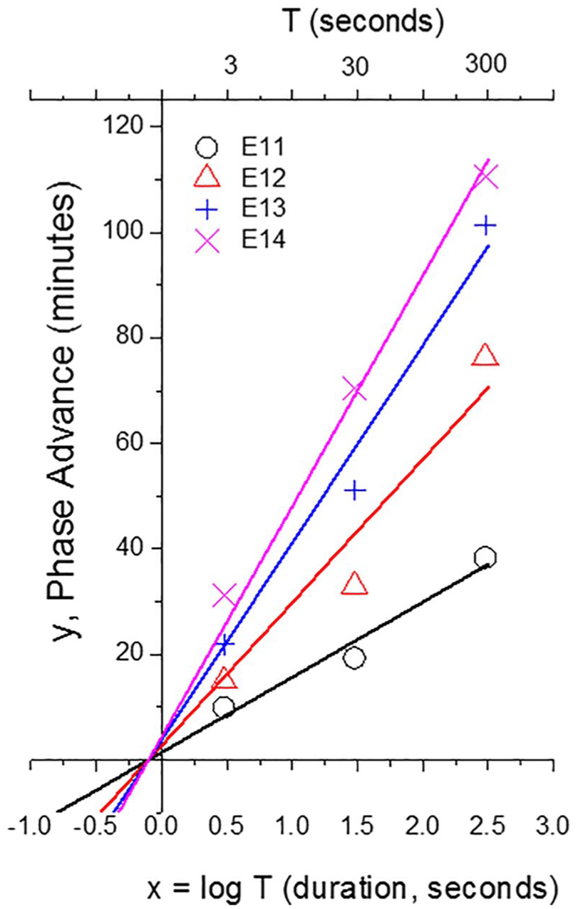
Fits to golden hamster phase advance data (minutes) as a function of stimulus duration (T, sec) transformed into x = log T (reproduced from Nelson and Takahashi, 1991). Constrained linear/log fits (with a universal ${\widehat{T}}_0$ = 0.79 sec).

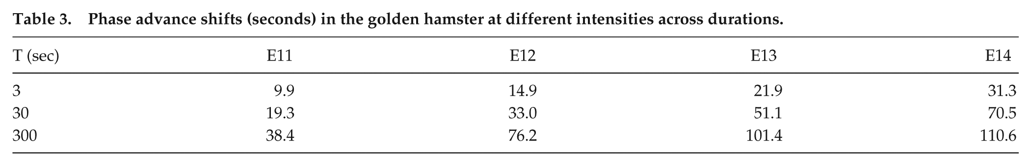
The Naka-Rushton functions allow calculating the shift, y, for any I and any T; we chose their 4 intensities (I) (E11, E12, E13, and E14) and 3 durations (T) (Table 3). We switch the emphasis from the original study (i.e., effect of different intensities at each duration) to the effects of different durations at each intensity. Therefore, our first use was to test whether for intensity I, the linear/log dependence for short T as described above for humans would also be observed in hamster phase-advance shifts. We conducted an unconstrained linear fit of phase shift, y, versus log T to determine the slope, m(I), and intercept T₀(I) for each intensity (I) from Table 3, with results as reported in Table 4. Overall, for the full range of I, the average root mean square deviation (RMSD) was 4.04 min (which is within the 6-min range); we return to this RMSD value below.

Table 3.

Phase advance shifts (seconds) in the golden hamster at different intensities across durations.

T (sec)	E11	E12	E13	E14
3	9.9	14.9	21.9	31.3
30	19.3	33.0	51.1	70.5
300	38.4	76.2	101.4	110.6

Table 4.

Results of unconstrained and constrained linear/log fits to golden hamster phase advance data.

	Unconstrained Fits				Constrained Fits
I	m	x0	T0	RMSD	m	x0	${\widehat{T}}_0$	RMSD
E11	14.2	−0.11	0.79	2.26	14.3	−0.10	0.79	2.26
E12	30.7	0.13	1.34	5.94	27.2	−0.10	0.79	6.75
E13	39.7	0.01	1.03	4.98	37.5	−0.10	0.79	5.40
E14	39.6	−0.31	0.49	0.20	43.8	−0.10	0.79	3.78
Mean ± SD		−0.07 ± 0.19	0.91 ± 0.36

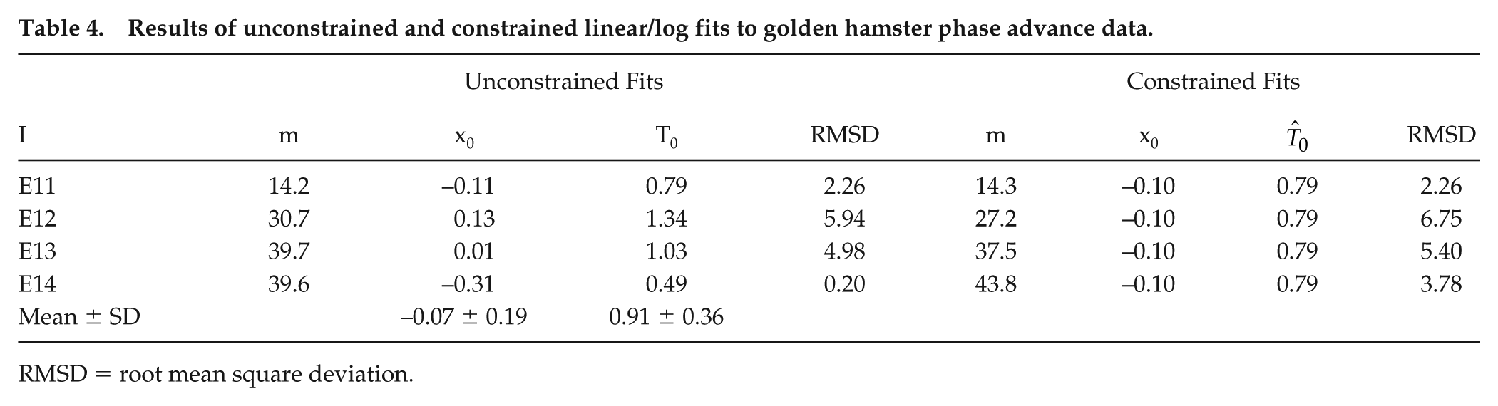
RMSD = root mean square deviation.

Each linear/log fit is characterized by the time parameter, T₀. Over the selected I range of 1000:1, T₀ ranges from 0.49 to 1.34 sec, which leads us to an important conjecture: perhaps there is an underlying ${\widehat{T}}_0$ independent of I such that the observed range in T₀ arises solely from noise in the data. This conjecture set us on a search for a suitable constraining ${\widehat{T}}_0$ . We realized that imposing any such constraint on T₀ across the 1000:1 range of I must necessarily increase the RMSD; therefore, our aim was to find a ${\widehat{T}}_0$ that minimizes RMSD from the data and maintains an overall RMSD of 6 min or less. We therefore conducted a single linear regression using the data across all intensities (rather than individual fits to each light intensity), which resulted in an overall ${\widehat{T}}_0$ = 0.79 sec (Figure 4) and an overall RMSD value of 4.85 min, which is within our imposed 6-min range.

With the sole parameter of the linear/log function, T₀, constrained to a single ${\widehat{T}}_0$ over the entire intensity range, m(I), the influence that light intensity I has on phase shift is contained within the multiplying coefficient, m(I) (Table 4, constrained fits). Using this, we discover that the values of m(I) follow a simple logistic function (Figure 5). For comparison, Figure 5 also includes the original m(I) values for the unconstrained linear fits as reported in Table 4. Imposing a constraining $T_0$ cleans up the presentation of m(I), revealing the innate character of the primary data.

Figure 5.

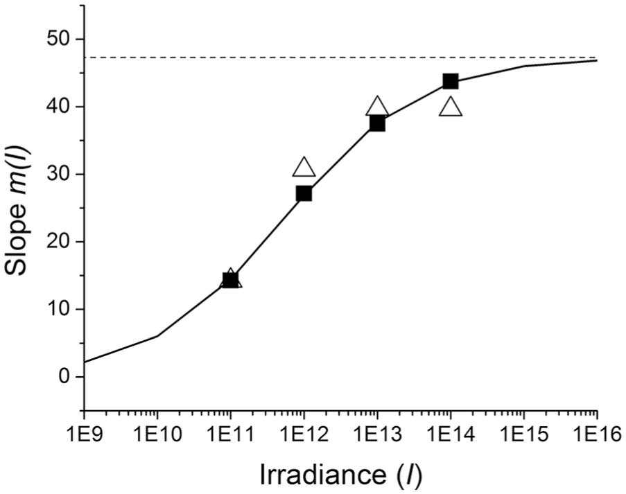
Relationship between intensity (or irradiance, I) and slope m(I) using values from Table 4 (derived from linear fits with universal ${\widehat{T}}_0$ ). The solid line is a logistic fit to these values; the horizontal dashed line denotes the asymptote of this fit. Slope values derived from the unconstrained fits (Table 4) are included for comparison (open triangles).

We now rewrite equation 1 in a more powerful way:

$$y\left(I,T\right)=m\left(I\right)\left(\log T-\log {\widehat{T}}_0\right)$$

(3)

Equation 3 suggests that the dependence of shift on stimulus intensity, m(I), and stimulus duration T₀ can be factored into 2 independent functions, which is known as product separability. We have already discussed earlier that the duration (time) function embodied in equation 1b (which is linear/log) shows no saturation. In contrast, Figure 5 indicates that the intensity function m(I) does indeed saturate for (intensity) I → ∞ when m(I) = 47.5 min, supporting our claim in equation 3 that duration (time) and intensity factors are independent influences on yield.

We are now able to compare our model predictions (equation 3, using the constrained fit values of $m\left(I\right)$ and ${\widehat{T}}_0$ as reported in Table 4) to the raw data from Nelson and Takahashi (1991) that we have reproduced in our Figure 3. Our model predictions (equation 3) reveal that the asymptotic shift values for T = 3, 30, and 300 sec are 27.4, 74.9, and 122.4 min, respectively. Note that while our product-separable representation fits the Nelson and Takahashi data quite well for T = 3 and 300 sec, the data for T = 30 sec consistently lie below model predictions. The original Naka-Rushton fit to T = 30 sec in figure 5 of Nelson and Takahashi is better than our fit, but it appears in that paper that the upper asymptote has been constrained to equal the upper asymptote found for T = 3600 sec (discussed above), whereas we do not constrain the upper asymptote in our fit for T = 30 sec.

In summary, using this data set, we were able to demonstrate the following:

• A linear/log relationship can represent the relationship between response (phase-advance shift, y) and duration, T, for each intensity, I, individually.

• The sole time parameters, T₀, of the individual linear/log processes could be constrained to a single value, ${\widehat{T}}_0$ , that is independent of stimulus intensity, I.

• The response, y, can be represented as the product of an intensity function, m(I), and a duration function, $\log T-\log {\widehat{T}}_0$ .

Short and Long Stimulus Duration Phase Shifting in Mouse

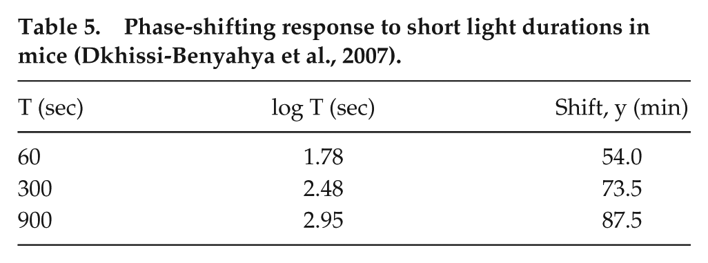
For a long time, we despaired of finding studies of nonhuman phase shifting by light that could be compared with our human short-duration and long-duration stimuli data. Then, we discovered the data of Comas et al. (2006). Because Comas et al. used no stimulus shorter than T = 60 min, we additionally sought a data source that could confirm and quantify the linear/log (short T) behavior for the mouse, and found one in the 2007 report by Dkhissi-Benyahya et al. (2007); a report by the same group (Dollet et al., 2010) mostly duplicates these data points and is not included here. These short T data are sparse, as they were intended to provide a baseline validation of their experimental protocol, which primarily addressed phase shifting in mice lacking mid-wavelength cones. The stimulus durations tested were 1-, 5-, and 15-min light exposures (480-nm monochromatic light at 2.8 × 10¹⁴ photons/cm²/s). We scaled the delay shifts from their figure 5 to generate our Table 5. These points generate an excellent linear/log fit with T₀ = 0.79 sec and m = 28.6 min, with an adjusted R² = 0.99, as observed in Figure 6B. We compare these parameters to our human data, where T₀ = 0.65 sec (0.011 min) and m = 23.13 min.

Table 5.

Phase-shifting response to short light durations in mice (Dkhissi-Benyahya et al., 2007).

T (sec)	log T (sec)	Shift, y (min)
60	1.78	54.0
300	2.48	73.5
900	2.95	87.5

Figure 6.

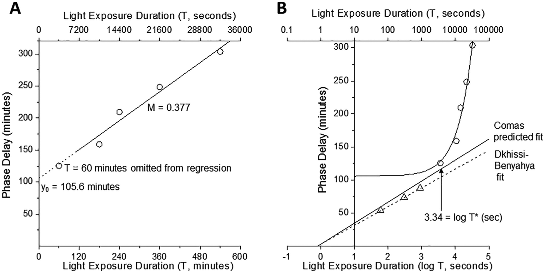
(A) Phase-delay shifts in mouse (open circles; from Comas et al., 2006) in response to long-duration stimuli. The solid line indicates a linear/linear fit to the long-duration data. The data point at T = 60 min was omitted from the fit, as indicated by the extrapolated dashed line. (B) The phase-delay data over long-duration stimuli (open circles) are plotted in a linear/log manner against phase-delay shifts in mouse in response to short-duration stimuli (open triangles; from Dkhissi-Benyahya et al., 2007). The solid line to long duration represents the same fit as plotted in panel A. The dashed line represents the fit of the short-duration data, and the solid line fit over this same range represents the fit that would be predicted by the long-duration data.

Now we are prepared to address the torrent of data in Comas et al. (2006). As shown in their figure 1, they selected 7 stimulus durations of 1, 3, 4, 6, 9, 12, and 18 h. Light pulses were generated by white fluorescent tubes and achieved an intensity of ~100 lux (~145 mW/m² at the cage floor level). We report in our Table 6 the maximum delay shifts (in minutes) for the relevant T durations (also in minutes) as taken from their table 1 (Comas et al., 2006). We have added the values for log T (in seconds) for use in our Figure 6B. We treated these data in the same way we treated the human long-duration stimuli data above: we ignored the data at T = 60 min (considering it to be transitional, as we discuss further below) and fitted a linear regression to the remaining 4 points, obtaining y₀ = 105.6 min and M = $\frac{dy}{dT}$ = 0.38 with an adjusted R² = 0.94. This fit is shown in Figure 6A, which is comparable to Figure 1A for the human data. We recall that a similar regression fit to the human data yielded y₀ = 76.8 min and M = $\frac{dy}{dT}$ = 0.24 with an adjusted R² = 0.95.

Table 6.

Phase-Shifting Response to Long Light Durations in Mice (Comas et al., 2006).

T (min)	log T (sec)	Shift, y (min)
60	3.56	125.4
180	4.03	159.0
240	4.16	209.4
360	4.33	248.4
540	4.51	303.6

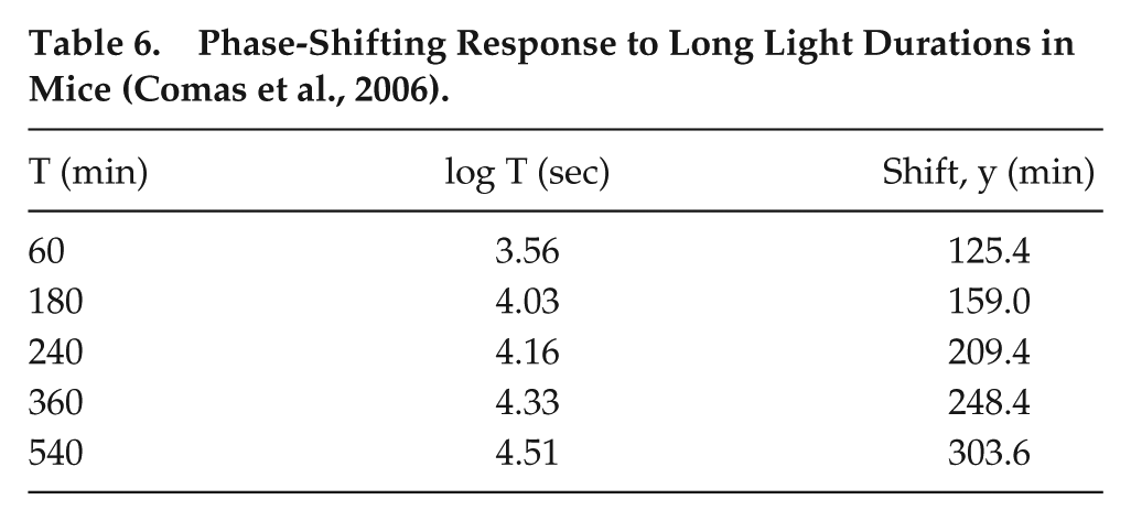
At this point, we audaciously try to predict short-stimulus duration data for Comas et al., if they had undertaken such studies using the same handling and lighting procedures as they did for their long stimulus duration data. The key to such prediction is y₀, which is a window into short T from long T. The short T parameter we seek to predict is m = $\frac{dy}{d\log T}$ .

The data we have in hand that transcends the short-T to long-T transition is the human phase-delay shift data. We propose that

$$m_{Comasmouse}=m_{human}\frac{y_{0,Comasmouse}}{y_{0,human}}$$

From the values for human and mouse that we have derived, we obtain

$$m_{Comasmouse}=23.13\frac{105.6}{76.8}=31.8\min$$

For $T_{0,Comasmouse}$ , we would expect T₀ = 0.78 sec as derived from the Dkhissi-Benyahya et al. (2007) mouse data to apply directly. We have added to Figure 6B this short-T estimate for the Comas et al. (2006) data and note that the predicted slope m = 31.8 is close to the slope m = 28.4 observed in the Dkhissi-Benyahya et al. (2007) data.

We are now in a position to estimate the characteristic stimulus duration, T^*, for the transition in mouse from the linear/log function to the linear/linear function. Using the predicted short-T slope m = 31.8 min and the observed long-T slope M = 0.38 from the Comas et al. (2006) data, we find that

$$T^{*}=\frac{\tilde{m}}{M}=\frac{\raisebox{1ex}{$m$}\!\left/ \!\raisebox{-1ex}{$2.303$}\right.}{M}=\frac{13.81}{0.38}=36.6\min$$

which is remarkably close to T^* = 37.2 min predicted for humans.

The Leaky Integrator Model: A Bridge Between Extremes of Responses

The data that we have just analyzed in multiple species appear to have a discontinuity: for short light pulses (i.e., on the order of a few minutes), there is the linear/log process with a declining yield, while for long pulses, the resetting response is a linearly increasing function of T but with a small yield. An essential feature of the Figure 1B presentation is that the 2 curves do not intersect. Although prior discussions of the data in Figure 1B have modeled the dynamics using a single 4-parameter logistic function (Chang et al., 2012; Rahman et al., 2017), in the leaky integrator analysis formulated below, we propose to embrace these disparate behaviors as limiting cases of a single first-order dynamical system defined by a time constant, B⁻¹, as an alternative model. Before we can develop the leaky integrator model, however, we need to address a fundamental question that we deferred to this section: in defining the long-T linear incremental function, may we use all 4 data points, T ≥ 60 min, or should we restrict the range to the 3 data points T >60 min (corresponding to T ≥ 150 min in our data set)?

• In case 1 (3 data points, T ≥ 150 min), y₀ (intercept) = 76.8 min, adjusted R² = 0.95, M (slope or yield) = 0.27 min of phase shift per minute of light exposure.

• In case 2 (4 data points, T ≥ 60 min), y₀ (intercept) = 84.4 min, adjusted R² = 0.96, M (slope or yield) = 0.24 min of phase shift per minute of light exposure.

Thus, although the addition of the data point T = 60 min changes both the intercept and yield, we cannot choose one over the other on statistical grounds. A decision can be made only when the linear/log curve for short T is considered.

In our discussion of the human data, we described the linear/log function in equation 1b as $y=m\left(I\right)\log \frac{T}{T_0}$ . The fit to the 3 short-T data points (T = 15, 120, and 720 sec ) yields m = 23.13 min and T₀ = 0.65 sec with an adjusted R² = 0.82. We can now convert equation 1a to the natural logarithm:

$$y=\tilde{m}\left(I\right)\left(\ln T-\ln T_0\right)$$

(1d)

where $\tilde{m}\left(I\right)=\frac{m\left(I\right)}{2.303}=10.04$ min (where ln 10 = 2.303 when we convert from log to ln). Now, as Figure 1B shows and as noted above, the short-T and long-T processes do not intersect, but they come close. Earlier, we undertook to quantify the stimulus duration for which they are closest. This is the value of T for which the functions have matching time derivations. For equation 1d, the matching time derivation is

$$\frac{dy}{dT}=\frac{\tilde{m}\left(I\right)}{T}$$

(4)

where both y and $\tilde{m}\left(I\right)$ have dimensions in minutes. We chose the dimension for T to be minutes so that $\frac{dy}{dT}$ matches M (i.e., for long T) dimensionally. We then designated the closest approach for the 2 functions as T^* in minutes. Now, for case 1 (3 points):

$$M=\frac{\tilde{m}\left(I\right)}{T^{*}}\mathrm{or}{T}^{*}=\frac{\tilde{m}\left(I\right)}{M}=\frac{10.04}{0.27}=37.19\min$$

For case 2 (4 points):

$$T^{*}=\frac{\tilde{m}\left(I\right)}{M}=\frac{10.04}{0.24}=41.83\min$$

The message here is that this parameter T^*, which characterizes the transition process, is surprisingly close to 60 min, which places that data point in the transition zone. Therefore, case 2 (with 1 point at ~60 min) was rejected from the long-T fit.

It is with these findings in hand, therefore, that we elected in Figure 1B to show the case 1 (3 points) representation for the long-T function and added a marker for T^* = 37.19 min (T^* = 2260 sec, x = log T = 3.35). In the leaky integrator analysis below, we suggest that T^* is equivalent to the leaky integrator time constant.

We now focus on this transition between behaviors for short T and long T.

Origins

There are some key points to suggest a leaky integrator type of physiology:

• For short T, there is a linear/log response, for which yield (phase shift per unit of stimulus duration) is initially very high (139.2 min of phase shift for each minute of light exposure in humans, as noted above) and then declines inversely as the stimulus duration (T) increases (see inset of Figure 1A). This decline is continuous and approaches zero.

• For long T (T >60 min), however, the yield does not asymptote to 0 but instead maintains a steady nonzero yield with increasing light exposure duration (about 0.27 min [~16 sec] of phase shift per minute of light exposure in humans). Although the yield resulting from long stimulus durations is much lower than for short stimulus durations, when the stimulus duration is long, the sum of the resulting incremental phase shifts can be substantial.

• Between the “inverse T” linear/log relationship of short-duration light pulses to the steady yield linear/linear relationship of long-duration stimuli, there appears to exist a transition.

The transition to a steady yield implies that the integrator process is imperfect. For a perfect integrator, yield would continue to decrease over time as the duration of the stimulus (T) increases. Our results show that the integrator reaches a steady state at some finite value (i.e., the yield fails to decline with the inverse of T as T increases). Therefore, we chose to model the process as a “leaky” integrator. The example of a leaky integrator taught in mathematics classes is a reservoir with in-flowing water. If the reservoir is a perfect integrator, the total (i.e., integrated) amount of water in it will continue to rise indefinitely. If the reservoir leaks, then the total amount of water may (in some circumstances) reach a fixed level. The analogy to phase resetting would be the sum of the photons as measured by stimulus duration (T; instead of in-flowing water) being inversely related to the rate of the change of the phase shift (instead of amount of water). Note that a strict photon counter-type physiologic response cannot produce this observed behavior. The yield is inversely related to the rise of the total amount of water in the reservoir. For a perfect integrator, the yield will decrease because the total amount of water in the reservoir increases. For a leaky integrator, the amount of the leak is related to the amount of water in the reservoir, and therefore the yield will reach a steady state (which may be zero if it reaches a fixed level) as water flows both in and out.

The Imperfect “Leaky” Integrator

To keep the mathematics simple, we envision that the process begins at the onset of integration, T = 0. Let R be the output of the (defective) integrator and consider

$$\frac{\mathit{d}\mathit{R}}{\mathit{d}\mathit{T}}=1-\mathrm{BR}$$

(5)

If B = 0, then $\frac{\mathit{d}\mathit{R}}{\mathit{d}\mathit{T}}$ = 1 and R is simply T itself, that is, a perfect integrator. A positive value for B implies outflow from the reservoir, R (i.e., a “leak”). As R increases, so does outflow. Finally, a balance ( $\frac{\mathit{d}\mathit{R}}{\mathit{d}\mathit{T}}$ = 0) is reached when BR = 1: outflow matches inflow. The entire transient process is described by a particular integral of equation 5:

$$R=B^{-1}\left(1-e^{-BT}\right)$$

(6)

Note that at T = 0, R = 0 and that R = B⁻¹ is the asymptotic value for R as T increases. Both R and B⁻¹ are time parameters, and B is therefore a rate parameter. As we approach the asymptote, the value of B characterizes the rate of approach. For what is to follow, we comment that, parameters aside, the functional dependence of R on T is simply $1-e^{-BT}$ .

In describing the linear/log process, we wrote the yield function in equation 4 as $\frac{dy}{dT}=\frac{\tilde{m}\left(I\right)}{T}$ , where $\tilde{m}\left(I\right)$ = $\frac{m\left(I\right)}{2.303}$ and T is the perfect integrator. For the leaky integrator, we replace T by R(T):

$$\frac{1}{\tilde{m}\left(I\right)}\frac{dy}{dT}=\frac{1}{R\left(T\right)}=\frac{B}{1-e^{-BT}}$$

(7)

The open integral of equation 7 is

$$\frac{\mathit{y}}{\tilde{\mathit{m}}\left(\mathit{I}\right)}=ln\left(e^{BT}-1\right)$$

(8)

We observe that for BT >> 1, $\frac{\mathit{y}}{\tilde{\mathit{m}}\left(\mathit{I}\right)}\to BT$ , which is the linear/linear (long T) process.

We understand that the linear/log process (short T) originates at T₀. Consequently, we convert equation 8 to a definite integral originating at T₀:

$$\frac{\mathit{y}}{\tilde{\mathit{m}}\left(\mathit{I}\right)}=ln\left(e^{BT}-1\right)-ln\left(e^{B{T}_0}-1\right)$$

(8a)

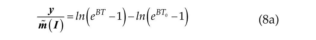
Equation 8a represents the complete leaky integrator solution and introduces a single parameter, the rate constant B. It is easier to interpret this model in terms of the time constant, B⁻¹, which we will now do.

Limiting Cases

Note that B⁻¹ establishes a time scale for the transition between the linear/log process (short T) and the linear/linear process (long T). We look at equation 8a for these 2 limiting cases. In the context of human data, B⁻¹ lies somewhere between T = 12 and T = 60 min (Figure. 1).

Limiting case 1, at short T, where T<< B⁻¹ and T₀ << B⁻¹: in this case, $(e^{BT}-1)\to BT$ and equation 8a becomes

$$\frac{\mathit{y}}{\tilde{\mathit{m}}\left(\mathit{I}\right)}=ln\left(BT\right)-ln\left(B{T}_0\right)$$

(9a)

$$=ln\left(T\right)-ln\left(T_0\right)=\ln (\frac{\mathit{T}}{{\mathit{T}}_0})$$

(9b)

which is simply the linear/log relationship as in equation 1c.

Limiting case 2, at long T, where T >> B⁻¹ or BT >> 1: in this case, $ln\left(e^{BT}-1\right)\to BT$ . Since BT₀ << 1, however, $ln\left(e^{B{T}_0}-1\right)\mathrm{remains}\ln \left(B{T}_0\right)$ , as in the short T case.

Now, equation 8a becomes

$$\frac{y}{\tilde{m}\left(I\right)}=BT+ln\left(\frac{1}{B{T}_0}\right)$$

(10)

or

$$y=\left(\tilde{m}\left(I\right)B\right)T-\tilde{m}\left(I\right)\ln \left(B{T}_0\right)$$

(10a)

which we rewrite simply as

$$y=AT+y_0$$

(11)

the familiar linear/linear function.

Evaluating the “Leak” Time Constant

Since A (the slope in equation 11) is now seen simply as $\tilde{m}\left(I\right)B$ , we can evaluate B⁻¹ as

$$\frac{1}{B}=\frac{\tilde{m}\left(I\right)}{M}=\frac{10.04}{0.27}=37.19$$

(11a)

using values derived from the human data. This is exactly the stimulus duration, T^*, for which the linear/log and linear/linear functions had their closest approach (i.e., matching time derivatives) in the human phase-delay data.

We must note that the paired equations 10 and 11 also embody a second equivalence:

$$y_0=-\tilde{m}\left(I\right)\ln \left(B{T}_0\right)=\tilde{m}\left(I\right)\ln \left(\frac{B^{-1}}{T_0}\right)$$

(11b)

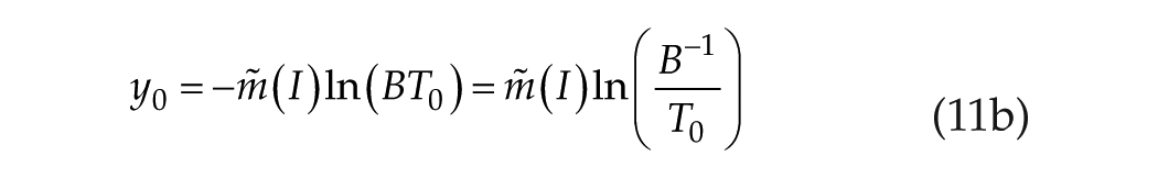
which may be solved for B⁻¹ as follows:

$$B^{-1}=T_0{e}^{\frac{y_0}{\tilde{m}(I)}}$$

(11c)

Just as equation 11a provides an estimate of B⁻¹ from the time derivatives embodied in the asymptotic functions, equation 11b incorporates the data provided by the intercept y₀. We now examine equation 11b further.

In equation 11b, the units of B⁻¹ and T₀ must match. We choose units of minutes, in which case T₀ becomes T₀ = 0.011 min (0.65 sec). Since we already have a solid estimate of B⁻¹ = 37.19 min from equation 11a, we use this along with T₀ and $\tilde{m}\left(I\right)$ = 10.04 min to calculate an estimate of y₀ (i.e., the phase shift at T₀) via equation 11b. We find this to be y₀ = 81.5 min. The original linear regression to the 3 longest-duration stimuli derived from the human data gave y₀ = 76.8 min, which is 7% less than this estimate. If y₀ is 76.8 min (from the human data rather than from equation 11a,b), then B⁻¹ is 22.7 min (equation 11c), which is a 40% reduction over the estimate from equation 11a. Thus, as expected from a log or exponential (not linear) function, a 7% reduction in y₀ results in a 40% reduction of B⁻¹.

We understood when y₀ was first recognized in the human phase delay data that it was an embodiment of all the high-response sensitivity to early photons. Equation 11b contains the 2 parameters T₀ and $\tilde{m}\left(I\right)$ that characterize the early (short-T) linear/log process. That equation 11b predicts y₀ to within 7% is quite remarkable. Equation 11c, however, proves to be a very inaccurate tool for evaluating B⁻¹. We must rely solely on equation 11a for evaluating B⁻¹ until more data are available.

Discussion

Summary

We have undertaken to describe the responsiveness of the circadian pacemaker in several mammalian species with data that include the wide range of stimulus duration from 15 sec to 6.5 h within a single experimental protocol. We have made several observations from these data. First, in the first few minutes of light exposure, the circadian system is maximally responsive. Second, the system continues to be responsive to longer-duration light stimuli, although at a reduced phase-resetting yield. Third, these properties are common across several mammalian species. Finally, the impact of intensity and duration on the resetting response appears to be functionally separable; that is to say, the temporal dynamics of the phase-resetting response to light stimulus duration are independent of intensity. These findings, if confirmed by further experiments, have important practical implications in terms of the design of lighting regimens to reset the mammalian circadian pacemaker.

Let us once again summarize the assumptions embedded within the linear/log concept. First, the entire duration dependence of shift response within the short-T linear/log regime (be it delay or advance shift) appears to be well described by a single parameter, T₀. We find the value of T₀ of ~0.7 sec to be remarkably similar across mammalian species. Second, extrapolation of data downward to T₀ suggests that no overt shift response will be observed for a single light stimulus when T < T₀. Third, yield (added shift per element of added stimulus duration) is very high for T of approximately 1 sec but decreases dramatically as T is extended. Yield does not decline gracefully (exponentially) in this regime but is actually driven downward inversely with T. Finally, based on the remarkable data from Nelson and Takahashi (1991), spanning both 3 log units of stimulus duration T and 4 log units of intensity I, we suggest that shift response can be factored into the product of distinct functions for duration T and intensity I, where the duration function is linear/log and the intensity function follows a traditional Naka-Rushton relationship.

Our findings on the long-T linear/linear response to stimuli in excess of 1 h, as observed in both human and mouse data, is somewhat protocol dependent. First, this linear/linear response depends on operating within the phase-delay region of the traditional PRC. Second, the light stimulus should be sufficiently strong, such that the natural progression of the circadian pacemaker can be reversed (“shifted”) by the light stimulus, as occurs during a phase delay. The linear/linear relationship also requires that such reversal be achieved promptly, as the “prompt” data of Dkhissi-Benyahya et al. (2000) imply. Consider, for example, the consequence of a prompt realization of a 45-min phase delay (which we have measured on a subsequent circadian cycle) to a 2-min light pulse (Rahman et al., 2017). At the end of the light pulse, the pacemaker has been driven backward 45 min. In contrast, at the end of our 390-min light exposure, the pacemaker has been driven backward by only 183 min. These responses act to keep the pacemaker at, or near, the peak delay response of the PRC. In fact, the mouse data we take from Comas et al. (2006) are from a column they correctly labeled as “maximum delay,” indicating that these responses are indeed near the peak sensitive region of the PRC.

The wonderful phase-shift data resource of Nelson and Takahashi (1991) have led to several remarkable interpretations. First, we found evidence for a saturating logistic function of intensity, m(I), that supplies a multiplicative rate parameter to the temporal function (Figure 5). Second, we found evidence for a linear/log temporal function of duration T that appears to be universal for all intensities. For reasons that we laid out early in our analysis of the Nelson and Takahashi data, these principles extend to durations of 5 min and perhaps several minutes beyond but certainly not to 60 min. The linear/log function is characterized by a start time of T₀ = 0.79 sec independent of light intensity over the range of intensities available. By imposing a universal T₀ constraint on the entire Nelson and Takahashi data set (Figure 4), the overall response function y(I,T) is decomposed into a simple product of an intensity function, m(I), and a temporal function, (log T − log T₀). The intensity function saturates for large I (see Figure 5). The temporal function shows that the incremental response decreases inexorably for large T, but the accumulated response does not saturate over the range of durations studied.

The linear/log temporal function that we extracted from the Nelson and Takahashi (1991) data has proven to be extraordinarily useful. Both the gerbil data (for 3 sec ≤ T ≤ 285 sec) from Dkhissi-Benyahya et al. (2000) and our human data (for 15 sec ≤ T ≤ 720 sec) from Chang et al. (2012) and Rahman et al. (2017) were well fit by this function and gave T₀ values of 0.69 sec and 0.65 sec, respectively, which compare well to the universal T₀ = 0.79 sec derived from the Nelson and Takahashi (1991) data set.

Our central challenge is understanding human phase-delay shift data. We already knew that for T >60 min, the phase shift increases linearly with T up to T = 390 min (i.e., 6.5 h). When this linear function was projected back to T = 0 (giving an impossible phase shift of y₀ = 76.75 min for a light stimulus of 0 sec), it was clear that a significant shift had occurred before T = 60 min. This led us to initiate experiments for shorter-duration T (Chang et al., 2012; Rahman et al., 2017). These data revealed that there was a linear/log relationship for T < 60 min, similar to data that have been observed in other species. Now, we had 2 limiting behaviors: linear/log for T < 3600 sec (<1 h) and linear/linear for T > 3600 sec (>1 h). The mechanism that we proposed to approximate these limiting behaviors was the leaky integrator. The leaky integrator introduced only 1 new parameter (other than those already observed in the limiting cases): the rate constant, B, or what is more easily understood, the time constant B⁻¹.

The full leaky integrator solution, which embraces both limit cases, is defined in equation 8a. We have simplified equation 8a for the limit cases. The interesting feature is that these limit cases do not intersect; there is always a gap between the linear/log and the linear/linear portions for which the full leaky integrator equation must be used. We also have calculated the exact value for this gap as T = B⁻¹ as 37.2 min. In humans, we observe that the phase shift estimated by equation 8a at T = 37.2 min is ~87 min, whereas the extrapolation of the linear/log function to T = 37.2 min yields a phase shift of ~82 min. The difference is within the error limits, given the relatively small data sets.

In their figure 2B, Dkhissi-Benyahya et al. (2000) tried to fit a saturating Naka-Rushton equation to the c-fos–labeled cell density versus T. There is a widespread belief that response to increasing T must saturate, just as the response to increasing I does. The leaky integrator model is based on the concept that an incremental response saturates with increasing T, while a cumulative response does not until a different part of the PRC is reached. The leak rate, B, is also a purely temporal concept, and so we might expect that it, like T₀, will prove to be independent of I. As we cited above, the values of T₀ lie in a variation range of 7% across hamster, gerbil, and human. We look forward to learning whether the various B⁻¹ will be close to our estimate of 37.2 min, as more species are studied over a range of T that includes both the linear/log and linear/linear behaviors.

Caveats and Future Work

There is much work to be done to extend and validate the work presented here. First, given the small number of data points and variability in data, no one fit or model can currently be chosen as the most appropriate. Each mathematical fit has different physiological implications; presenting more than 1 possible physiological basis for the observed results can be used to develop new experiments to better define the physiology, since each will have different predictions under specific conditions. There is a paucity of phase-resetting data in the stimulus duration regime between 12 and 60 min for humans, between 15 and 60 min for mice, and between 5 and 60 min for hamsters. This regime is where we have predicted the transition from linear/log to linear/linear to occur. Specifically, we predict this transition to occur at T* = ~37.2 min. Future experiments in humans, mice, hamsters, and other species should therefore focus on light-stimulus durations within this regime using the same experimental protocols as in the existing studies to confirm the leaky integrator concept. In addition, experiments with light durations less than 3 seconds should be conducted in multiple species.

We have not considered here the physiological mechanism underlying the leaky integrator concept. We note, however, that the prompt resetting response observed in the short-duration linear/log regime may reflect a contribution of the cone photoreceptors in the retina. For example, a prior study from our group (in humans) observed that melatonin was more strongly suppressed during the first 30 min of exposure to monochromatic 555-nm light (a stimulus expected to activate primarily the cone photoreceptors) compared with monochromatic 460-nm light (a stimulus expected to activate primarily the melanopsin-expressing intrinsically photosensitive retinal ganglion cells [ipRGCs]), whereas melatonin was more strongly suppressed for stimulus durations longer than 30 min by the monochromatic 460-nm light (Gooley et al., 2010). A prompt response to stimulation of the cone photoreceptors and a sluggish but sustained response to stimulation of the melanopsin-expressing ipRGCs have also been observed in the pupillary light reflex (Alpern and Campbell, 1962; Bouma, 1962; Lucas et al., 2003; Gamlin et al., 2007; Mure et al., 2009; Gooley et al., 2012) and phase resetting (Panda et al., 2002; Hattar et al., 2003; Do and Yau, 2010; Gooley et al., 2010). Duration-response experiments that span both the short-T and long-T regimes are needed in both animals (i.e., rod/cone and melanopsin knockouts) and humans (monochromatic blue versus monochromatic green light exposures and/or in blind individuals with intact ipRGCs) to understand the contributions of the different photoreceptor systems to our leaky integrator concept.

In prior works, we have proposed other mathematical formulations to describe the phase-resetting effects of light (Kronauer et al., 1999; Kronauer et al., 2000; St Hilaire et al., 2007; Chang et al., 2012; Rahman et al., 2017). For example, the light preprocessor (Process L) of our mathematical model of the effects of light on the human circadian pacemaker (e.g., Kronauer et al., 1999; Kronauer et al., 2000; St Hilaire et al., 2007) was formulated as a nonlinear process in which the first 5 to 10 min of a light stimulus elicited a rapid increase in phase-resetting response followed by a slower increase in the rate of phase resetting after a critical light stimulus duration was released. The principles of the leaky integrator model introduced here are similar to this Process L formulation. Indeed, the distinctive shape of the leaky integrator model—logarithmic for short T, linear for long T—is similar to what is observed with integration of (1 − n(t)) from 0 to T, where n(t) is taken from Process L. However, the leaky integrator model incorporates new properties that have emerged from the available data since Process L was proposed, including (1) strong phase resetting in response to short stimulus durations (e.g., T = 15 sec and 2 min) in humans, (2) identification of the critical duration window within which the response transitions from a rapid increase in phase resetting to a slower rate of increase (i.e., between T = 12 and 60 min), and (3) discovery of the minimal stimulus duration T₀ at ~0.65 sec. In addition, (1) Process L does not have the property of the 2 regimes (log/linear and linear/linear) that we have identified, which is an important feature at short T that emerges from the data we have analyzed here, and (2) Process L would need significant reparameterization to generate the phase shifts observed at short T, and this reparameterization then fails to reproduce other properties of the effects of light on the circadian pacemaker (unpublished work). We have also previously used a 4-parameter logistic function to describe the relationship between the stimulus duration and phase-resetting response (Chang et al., 2012; Rahman et al., 2017). All 3 of these mathematical formulations provide a reasonable fit to the data, but given the sparsity of the data sets, it is not possible to distinguish statistically which one is the best. A comparison of these models to determine which model best represents the physiology should be done after additional experiments are performed.

Finally, here we have considered only the resetting response to a single light stimulus. In a prior study in humans, we reported that a single sequence of intermittent light (six 15-min bright-light pulses separated by 60 min of very dim light; 6.5 h total) yielded a phase shift that was 73% of the phase shift induced by a 6.5-h continuous bright-light stimulus despite representing only 23% of the continuous stimulus duration (Gronfier et al., 2004). Similar findings have also been reported in mice (Comas et al., 2007). More recently, Zeitzer and colleagues have demonstrated that sequences of 2-msec light flashes can elicit significant phase-resetting responses (Zeitzer et al., 2011; Najjar and Zeitzer, 2016). These findings suggest that the system is capable of integrating a series of consecutive light stimuli, even if they are very brief (i.e., shorter than our estimated T₀ value). The current version of our leaky integrator model cannot address the integration of the light input signal over intermittent exposures; further work is needed to understand this phenomenon. We further note that while our estimated T₀ value of ~0.7 sec, which represents the minimal stimulus duration at which a response is elicited, is not consistent with the findings of multiple millisecond flashes, it is consistent with the finding from Nelson and Takahashi (1991) that a single 3-msec pulse elicits no measurable response; to our knowledge, single millisecond flashes have not been tested in humans.

Conclusion

These findings highlight consistencies in the temporal dynamics of circadian resetting responses to single-duration light exposures across species and further challenge the notion of the circadian phase-resetting system as a photon counter. We look forward to the results of future experiments and modeling work.