Tau-independent Phase Analysis: A Novel Method for Accurately Determining Phase Shifts

Abstract

Estimations of period and phase are essential in circadian biology. While many techniques exist for estimating period, comparatively few methods are available for estimating phase. Current approaches to analyzing phase often vary between studies and are sensitive to coincident changes in period and the stage of the circadian cycle at which the stimulus occurs. Here we propose a new technique, tau-independent phase analysis (TIPA), for quantifying phase shifts in multiple types of circadian time-course data. Through comprehensive simulations, we show that TIPA is both more accurate and more precise than the standard actogram approach. TIPA is computationally simple and therefore will enable accurate and reproducible quantification of phase shifts across multiple subfields of chronobiology.

Accurate quantification of period, τ, and phase, φ, is a critical component of many studies of circadian rhythms. While multiple methods exist to quantify period (Dowse, 2009; Levine et al., 2002), ranging from relatively simple (linear regression of onset time, cosinor analysis) to more complex (chi-square periodogram, autocorrelation [Sokolove and Bushell, 1978]; discrete wavelet transformation, maximum entropy spectral analysis [Dowse, 2013; Leise, 2013; Leise and Harrington, 2011]), there are fewer options for estimating changes in phase. Phase analysis suffers from two large issues. First, methods to quantify changes in phase are less standardized, and thus potentially less reproducible, than those used for period analysis. Second, because phase shifts often coincide with changes in period (Comas et al., 2006; Pittendrigh and Daan, 1976), measurements of phase change can be affected by the magnitude of the coincident period change. Here we seek to address both of these issues by proposing a computationally simple but rigorous strategy for measuring phase shifts in multiple types of circadian data.

The measurement of a change in phase of a circadian pacemaker typically involves assessing how a pacemaker would have progressed if unperturbed (a null model) compared with how it actually progressed (Fig. 1). Within rhythmic data are overt phase reference points, such as onsets in actigraphy (Fig. 1A) or peaks in bioluminescence imaging (Fig. 1B). Phase reference points are a valuable property in the estimation of phase and period, as they represent a way to assess the progression of the pacemaker over time. Two successive phase reference points are assumed to occur one circadian cycle apart, and at those phase reference points the pacemaker is assumed to be at the same phase. Phase reference points are chosen for their recognizability and for the likelihood that their timing will remain consistent across changes to the overt, measured rhythm. For example, acrophase, the peak of a cosine fit to a circadian wave, is assumed to remain consistent even if the waveform broadens. In an experiment in which a pacemaker undergoes a potentially phase-shifting stimulus, a null model indicates the expected timing of these phase reference points after the stimulus, assuming no period or phase change (Fig. 1, A and B, dashed lines). The difference between the expected and observed timing of the poststimulus phase reference points can then be used to estimate the phase shift (Fig. 1, A and B, black arrows). If the stimulus also changes the period, however, the phase relationship between the observed poststimulus phase reference points and those of the null model is not consistent, and as such the difference between the real progression of the pacemaker and the null model varies by cycle, producing different measurements of the phase shift (Suppl. Fig. S1). One strategy for calculating phase shifts in the presence of period changes, most frequently used in actigraphy, involves altering the null model to include the change in period (Fig. 2). The original progression of the pacemaker, as well as the null model with the changed period, is depicted on the actogram as lines. The phase shift, Δφ, is then calculated as the distance between the 2 lines on the cycle after the stimulus occurs. This difference is represented in either circadian hours (relative to the period of the pacemaker after the stimulus) or in degrees. Using these units ensures that changes in phase can be compared across experiments.

Figure 1.

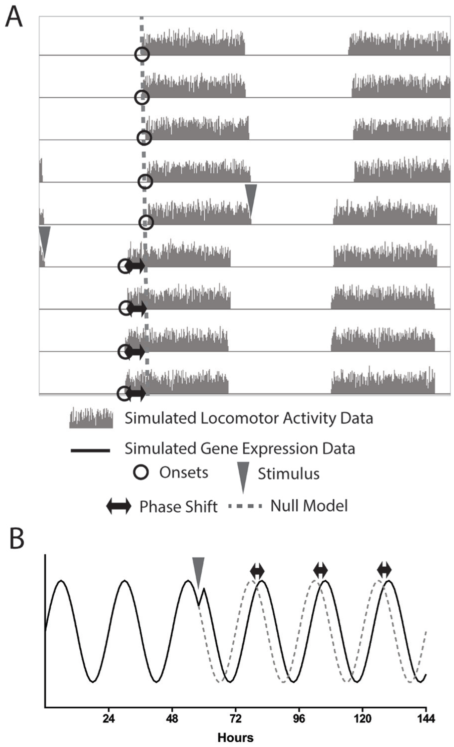
Schematic view of phase shift estimation. (A) A simulated actogram depicting a phase shift. Onsets before the shift are projected (dashed line) and the difference between the poststimulation onsets and the projection is taken to be the phase shift. (B) A simulated circadian waveform. A stimulus induces a phase delay, and the original trajectory of the wave is projected (dashed line). In both cases, the phase shift (black arrows) is calculated as the difference between the projected and the actual data.

Figure 2.

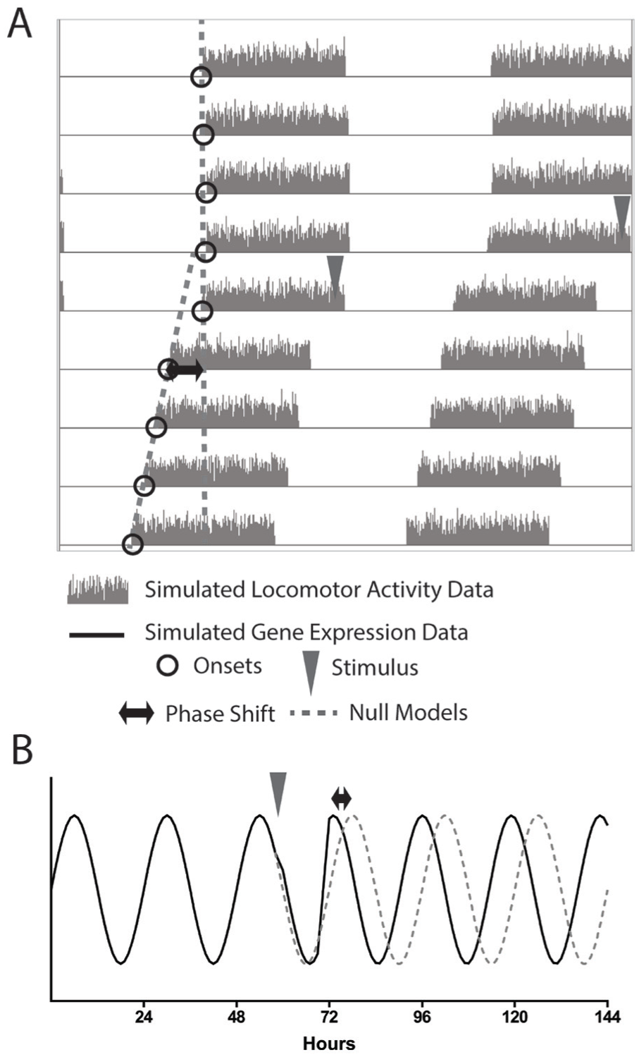
Period changes affect phase shift measurements. When a stimulus induces a period change along with a phase shift, the calculation must be adjusted. The phase relationship between the poststimulus phase reference points and the projected null model is not consistent from cycle to cycle (see Suppl. Fig. S1). To account for this, the phase shift is calculated as the difference between the projection of the prestimulus phase reference points and the linear fit of the poststimulus phase reference points. In this way, the change in period is included in the analysis.

Measuring the difference between the null model and the real data on the first cycle after the stimulus can be visualized as an altered version of the null model (Suppl. Fig. S2). In this view, the null model is projected 1 cycle, and then beyond that first cycle the slope of the model is altered to take into account the poststimulus period. Because this poststimulus null has the same period as the real poststimulus pacemaker, it maintains a stable phase relationship with the poststimulus phase reference points but is anchored to the prestimulus null model. The difference between the null model and the data on the first poststimulus cycle, which represents the phase shift (Fig. 2), is now recapitulated on every cycle (Suppl. Fig. S2). These representations are 2 depictions of the same phase shift estimation.

Because the prestimulus and poststimulus data are used to fit linear regression models, the respective periods are represented in the slope of the lines. This estimation therefore attempts to account for changes in period. In theory, if there were no change in phase, these pre- and poststimulus linear fits would intersect at the point of comparison (or, in the case of the altered visualization, the lines would overlap), and the estimated phase shift would be 0. In practice, however, changes in period between the pre- and poststimulus cause systematic error in the measurement of the phase change (Fig. 3). When using this strategy, which we term the “actogram approach,” the estimated phase shift becomes more negative (i.e., toward a delay) as the period decreases and more positive (advance) as the period increases, regardless of whether the actual phase shift is a delay (Fig. 3, left) or an advance (Fig. 3, right) or whether there is no shift at all (Fig. 3, middle). The average magnitude of the error in the phase shift estimate is about half the magnitude of the change in period (e.g., a typical error of –0.5 h for a period change of –1 h).

Figure 3.

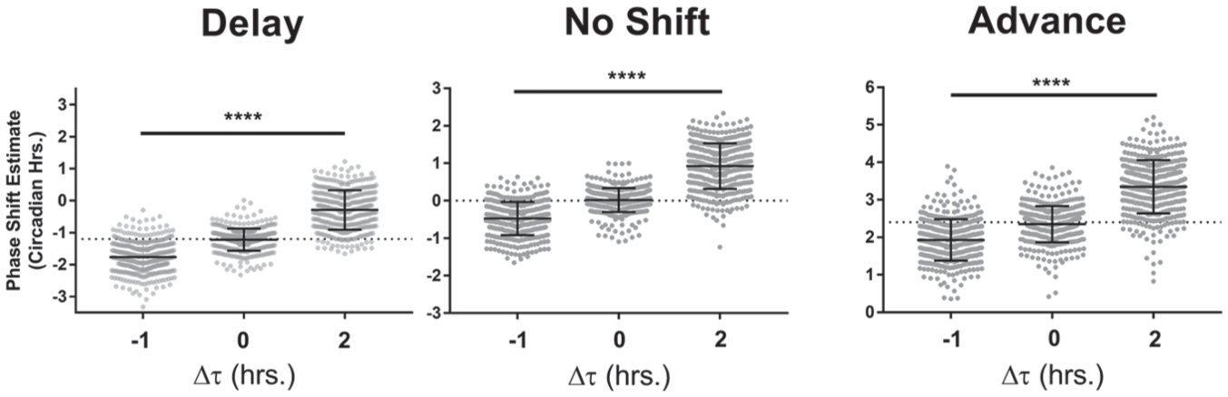
Period change affects phase shift estimates using the actogram approach. The phase shift estimate in circadian hours using the “actogram approach” is plotted against the magnitude of the period change in simulations with a phase delay (left, Δϕ = −1.2), no phase change (middle, Δϕ = 0), or a phase advance (right, Δϕ = +2.4). Each point represents 1 simulation of a circadian time-course. The dotted line represents the actual shift for that group of simulations. In all cases, period shortening produces a more delayed phase shift estimate and period lengthening produces a more advanced phase shift estimate. One-way ANOVA: **** corresponds to p < 0.0001. Δϕ values are represented in circadian hours. Error bars represent the standard deviation.

These inaccuracies are caused by an improper assumption about the relative time that the pacemaker undergoes a change in period, phase, or both. When measuring the difference between the 2 regression lines on the stimulus cycle, the actogram approach assumes that if the pacemaker’s phase and/or period was altered, that change occurred 1 full circadian cycle after the last prestimulus phase reference point. This assumption is made whether the stimulus occurs at the last prestimulus phase reference point, hours later, or nearly at the time of the next cycle’s phase reference point (Suppl. Fig. S2). The slope of the line for the null model begins operating under the poststimulus period parameter only at the first projected poststimulus phase reference point.

This assumption explains why, if the stimulus changes the pacemaker’s period, the actogram approach’s phase shift estimates are biased. The actogram approach does not account for the speed with which the pacemaker resets after a phase-shifting stimulus. This speed is a fundamental property of circadian pacemakers that has been measured experimentally. Classic experiments by Chandrashekaran (1967) and later by Pittendrigh (1981) established that the phase of the pacemaker resets within 1 h, at most. Since that time, the field has made substantial progress in establishing the molecular underpinnings of the clock in multiple organisms, including the molecular basis for the phase shift response (Shigeyoshi et al., 1997). While much remains unknown about the mechanism of the phase shift response, the work by Chandrashekaran and Pittendrigh demonstrates the timeframe within which the molecular resetting must occur. Because the expected phase response in the clock is achieved within at most 1 h, the molecular changes within the pacemaker that are required for that response are then known to occur within this window. The rapid induction of Per1 has been established as a portion of the molecular mechanism for pacemaker resetting within this timeframe (Shigeyoshi et al., 1997). This fast resetting is critical to accurately measuring phase shifts. If we assume that any changes in period and phase occur within an hour of the time of the stimulus (for stimulus lengths ≤1 h; for longer stimuli, see below), we can see a source of error in the actogram approach. The estimated phase shift includes not only the actual phase shift but also the change in period, weighted by the percentage of the cycle that occurs prior to the next phase reference point. Figure 4 illustrates this schematically, with 2 circadian waveforms with prestimulus periods (τ_pre) of 24 h undergoing an instantaneous period change (a period shortening of 2 h, poststimulus period τ_post of 22 h) but no phase change. The projection begins operating with the τ_post period parameter at the first projected poststimulus peak regardless of the stimulus time, which creates gaps between the projection and the poststimulus data that would be interpreted as phase shifts (dashed and solid lines, respectively; Fig. 4).

Figure 4.

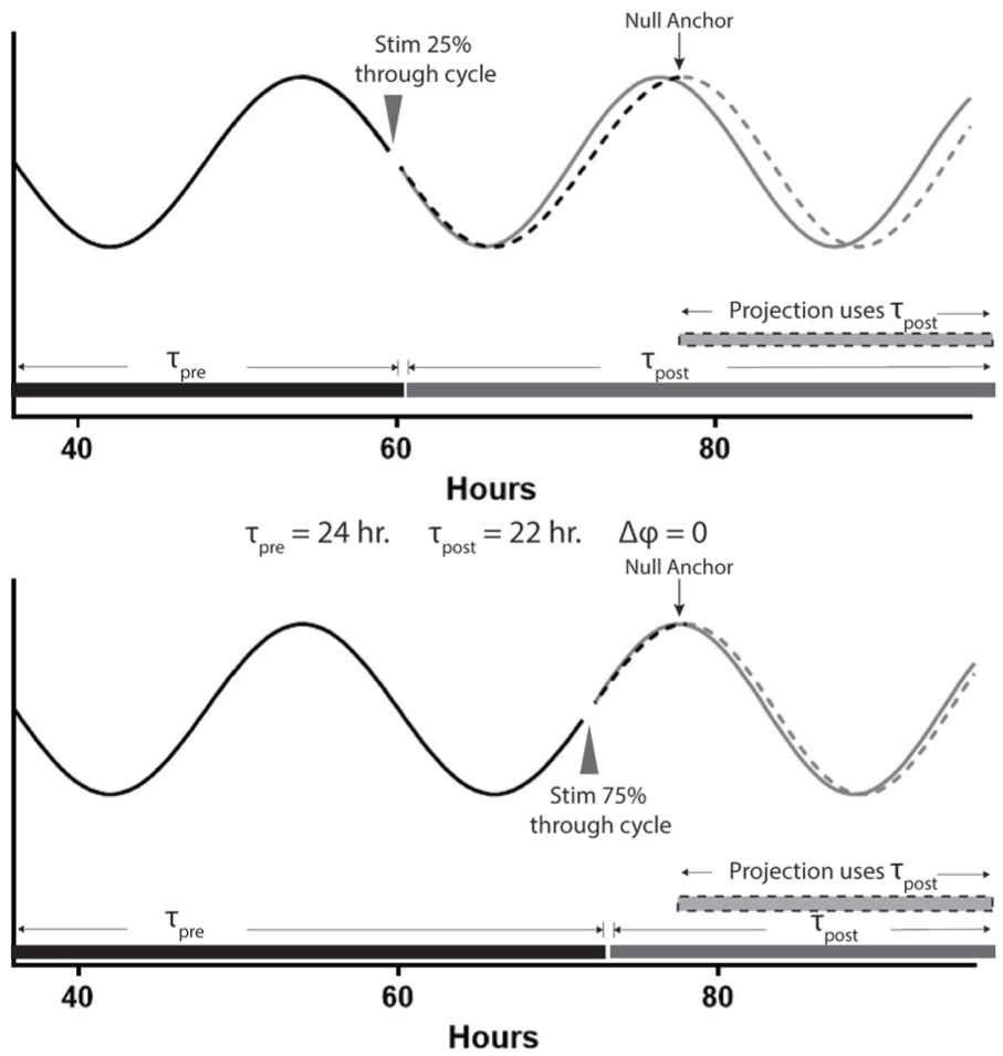
Schematic view of null model anchoring. When the poststimulus projection is anchored to the first projected poststimulus phase reference point (the “null anchor”), the projection begins operating under the τ_post parameter 1 full cycle after the last prestimulus phase reference point. This is the case whether the stimulus occurs early (top) or late (bottom) in the circadian cycle. In both examples, the stimulus does not cause a phase shift, but the period is shortened from 24 h to 22 h. Using the difference between the projected peak and the actual first poststimulus peak, the phase shift estimate is different between the 2 conditions. In top, the estimated phase shift would equal –1.5 h (0.75 * Δτ) and in bottom, –0.5 h (0.25 * Δτ), despite no phase shift having occurred.

To more accurately quantify the error in the actogram approach and to adjust for it, we assessed the relationship between the phase shift estimate and the time of stimulus relative to the last prestimulus phase reference point in a series of simulated phase shifts. In each simulation, the stimulus time is represented as the fraction of the circadian cycle that has elapsed when the stimulus occurred. We examined the error in the actogram approach’s phase shift estimate as a function of the stimulus time across 9 different conditions covering phase advances, delays, and no phase shift, as well as period lengthening, shortening, and no change in period (Fig. 5). We observed a clear relationship between the phase shift estimate and the stimulus time that was dependent on the change in period. When the period remained constant between the pre- and poststimulus conditions, using the actogram approach produced an accurate estimation of the phase shift (Fig. 5, middle row). When the period changed, the actogram approach was least accurate when the stimulus time was near the last prestimulus phase reference point and most accurate when the stimulus time approached 1 full circadian cycle later.

Figure 5.

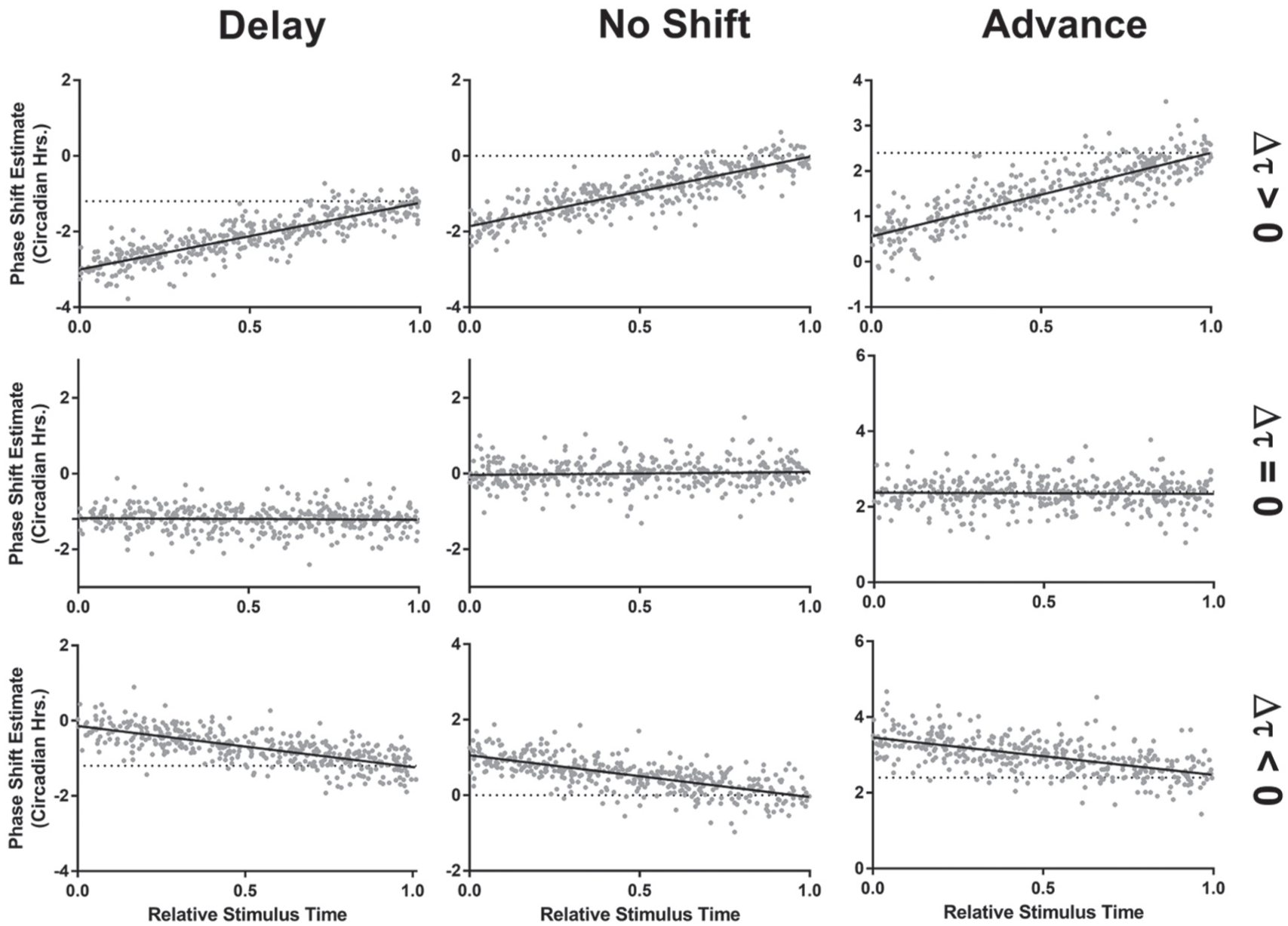
Relative stimulus time has systematic effects on the phase shift estimate using the actogram approach. Using the actogram approach, the relative time of the stimulus compared with the last prestimulus phase reference point has a predictable effect on the phase shift estimate, depending on the size and direction of the period change. When there is a period change (top and bottom rows), the estimate is least accurate when the stimulus occurs at or near the time of the last prestimulus phase reference point. This occurs whether there is a phase delay (left column, Δϕ = −1.2), no phase shift (center column, Δϕ = 0), or a phase advance (right column, Δϕ = +2.4). The direction of the error is dependent on the period change, with lengthening (top row, Δτ = +2) producing more negative (delayed) estimates and shortening (bottom row, Δτ = −1) producing more positive (advanced) estimates. When there is no period change, the actogram approach is generally accurate (middle row, Δτ = 0). Each point represents 1 simulation, and each black line shows a linear fit of estimated phase shift vs. relative stimulus time. Δϕ values are represented in circadian hours, Δτ values are represented in hours.

Methods

Tau-independent Phase Analysis (TIPA)

An ideal method for calculating phase shifts should be accurate regardless of the stimulus time and period change. We therefore sought to develop a method that would address the deficiencies of the actogram approach. The basis of tau-independent phase analysis (TIPA) is the creation of a null model of the pacemaker’s progression (represented by the time of occurrence of a chosen phase reference point) anchored appropriately to the actual time of phase and/or period change using the stimulus time described above (Fig. 6). This null model is based on the assumption that the pacemaker has undergone a change in period but no change in phase and that the change occurred exactly at the stimulus time. The differences between the observed times and the expected times according to the null model are then used to calculate the phase shift (Fig. 6, black arrows).

Figure 6.

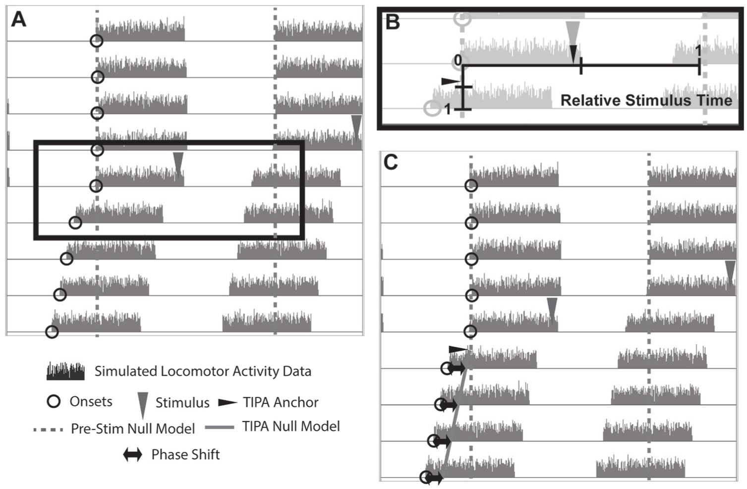
Schematic of tau-independent phase analysis. (A) A simulated actogram displaying a phase advance and a period shortening. (B and C) Using TIPA, the poststimulus null model (solid gray line) operates under the assumption that there is a period change but no phase change and that the period change occurred instantaneously at the time of the stimulus (gray triangle). The horizontal position of the stimulus is transposed vertically to show the TIPA anchor (black arrowhead in panel B). The sloped line representing the poststimulus null model is therefore anchored to a position along the prestimulus null model (gray dashed line) corresponding to the time of the stimulus. In panel C, the phase shift estimate (black arrows) for each cycle is shown as the difference in hours between the phase reference point (open circles) and the position of the TIPA null model (solid gray line) for that cycle.

The setup to this calculation is similar to the altered version of the actogram approach described above (Suppl. Fig. S2). Whereas the actogram approach anchors the poststimulus linear regression to the final prestimulus phase reference point, TIPA anchors its poststimulus null model to the stimulus time (Fig. 6, black arrowhead). The vertical position of the TIPA anchor can be determined by establishing the fraction of the circadian cycle that has elapsed by the time the stimulus occurs. In an actogram, time is represented both horizontally and vertically. Figure 6B shows the fraction of the circadian cycle horizontally from 0 to 1, with the stimulus occurring just before half the cycle is complete. The same 0 to 1 scale is then shown vertically as the height of a single actogram day. Again, the stimulus is represented, occurring just before half the cycle is complete. This is where the TIPA anchor is located, at the vertical position of the stimulus. The position of the anchor is intended to coincide with the instant of the period and phase change. For stimuli shorter than 1 h, the anchor is placed at the end of the stimulus. While maximum phase resetting occurs within 1 h of the onset of a stimulus (Shigeyoshi et al., 1997), period changes have been shown to align with the midpoint of the stimulus (Comas et al., 2006). For stimuli longer than 1 h, the TIPA anchor is therefore placed at the midpoint of the stimulus. Using this anchor, TIPA null estimates are then produced for each poststimulus cycle based on this origin at the time of stimulation, the fraction of the stimulus cycle that is operating under the poststimulus period parameter, and the poststimulus period. For each cycle, the difference between the actual poststimulus phase reference point and the TIPA null for that cycle is determined. The circular mean of these differences is the estimate of the phase shift (see below).

Simulations

To compare TIPA to the standard actogram approach, we simulated time-courses of circadian oscillations before and after a stimulus. Rather than simulating the full waveform, we directly simulated the times of phase reference points (e.g., activity onset times or peaks in bioluminescence). We varied multiple parameters of the simulated time-courses: the period of the oscillator before the stimulus, the number of cycles observed before and after the stimulus, the standard deviation of interreference point times, and the phase shift induced by the stimulus (Suppl. Table S1). For each combination of parameter values, we generated 100 simulations. The period of the oscillator prior to the stimulus was fixed at 24 h. In each simulation, phase-reference point intervals (produced separately for pre- and poststimulus epochs) were drawn from a Gaussian distribution with mean corresponding to the period of the oscillator and the given standard deviation. The fraction of the cycle elapsed at the time of the stimulus was drawn from a uniform distribution between 0 and 1. Any changes in period or phase induced by the stimulus were modeled as occurring instantly.

The simulations were imported into MATLAB where they were parsed into pre- and poststimulus subsets, with each subset being fit with a linear regression. The parameters from these regressions were used to make a set of predicted phase reference points for each simulation. For the phase shift estimate by the actogram approach, prestimulus and poststimulus predictions were compared on the cycle after, or the cycle of, the stimulus, as indicated.

TIPA Calculations

The phase-shift estimate of TIPA is calculated by measuring the difference, in circadian hours or degrees, between the observed poststimulus phase reference points and a set of poststimulus null estimates that we term TIPA_null. The times of the phase reference points and the TIPA_null points are represented in the elapsed time of the experiment, such that phase reference points that occur at projected ZT 12 each day would be represented as 12, 36, 60, 84 . . . . The TIPA_null for each poststimulus cycle i is calculated as follows:

$$TIP{A}_{null}\left(i\right)=t_s+{\tau }_{post}\cdot \left(i+f_s\right),i=0,1,2,\dots$$

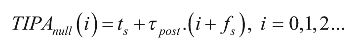
where t_s is the time of the stimulus and f_s is the fraction of the cycle that remains at the time of the stimulus. The difference (Δφ) between the observed poststimulus phase reference points (φ_{R, post}) and TIPA_null for each poststimulus cycle i is calculated as

$$\Delta \varphi \left(i\right)=TIP{A}_{null}\left(i\right)-{\varphi }_{R,post}\left(i\right).$$

The phase-shift estimate of TIPA is calculated as the circular mean of Δφ(i) for all values of i.

For values reported in this study, circular means were calculated using the CircStat MATLAB toolbox (Berens, 2009). Period parameters were estimated using linear fits of the phase reference points for the actogram approach and mean phase reference point intervals for TIPA. Because of the limitations of linear regression, it may be more suitable to estimate the period of the pre- and poststimulus data subsets using an external method, such as chi-square periodogram or autocorrelation, and then fixing the τ_pre and τ_post parameters to those values. In cases where limited numbers of cycles are available in the data, we recommend estimating the period as the mean interval between phase reference points.

Actogram Figure Generation and Data Availability

Actogram figures were simulated using sets of phase reference points selected from the simulations generated to test TIPA. The actograms values were created in MATLAB by creating a 10-day, 14,400-bin array with 12-h runs of randomly generated numbers 1 to 100 starting on each cycle with that cycle’s simulated onset time. Actograms were then formatted as TriKinetics monitor files and visualized using the ImageJ plugin ActogramJ (Schmid et al., 2011). Schematics of gene expression data were made using the curve generation function within Prism (GraphPad). Markings were then added in Adobe Illustrator. A spreadsheet for calculating the TIPA phase shift for all 3600 simulations generated for this analysis and the R code used to generate the simulations are available online at https://doi.org/10.6084/m9.figshare.5484916. An R package for calculating phase shifts using TIPA is available at https://github.com/hugheylab/tipa.

Results

To verify the accuracy and precision of the TIPA method, we analyzed the phase shift of 3600 simulations with known phase shift parameters (Suppl. Table S1). Two specific weaknesses of the actogram approach described above are the influence of a change in period (Fig. 3) and the relative time of stimulus (Fig. 5). Compared with the actogram approach, TIPA was robust against changes in period (Fig. 7A) and remained consistently accurate regardless of the time of stimulus (Fig. 7B). We also assessed the precision of the two methods in the case of no period change, where the relative stimulus time has no significant effect on the phase shift estimate of the actogram approach (Fig. 8). We found that TIPA was significantly more precise across phase delays (Fig. 8A), advances (Fig. 8C), and cases in which there was no phase shift (Fig. 8B). We further tested the precision of the two methods in cases where there was no change in period using simulations with various levels of noise and numbers of cycles (Suppl. Fig. S3). While both TIPA and the actogram approach showed lower precision in high noise simulations, the variance of TIPA’s estimates was significantly lower (Suppl. Fig. S3A). Neither the actogram approach nor TIPA showed reduced accuracy in simulations of 4 versus 5 poststimulus cycles, although TIPA had lower variance in each condition (Suppl. Fig. S3B).

Figure 7.

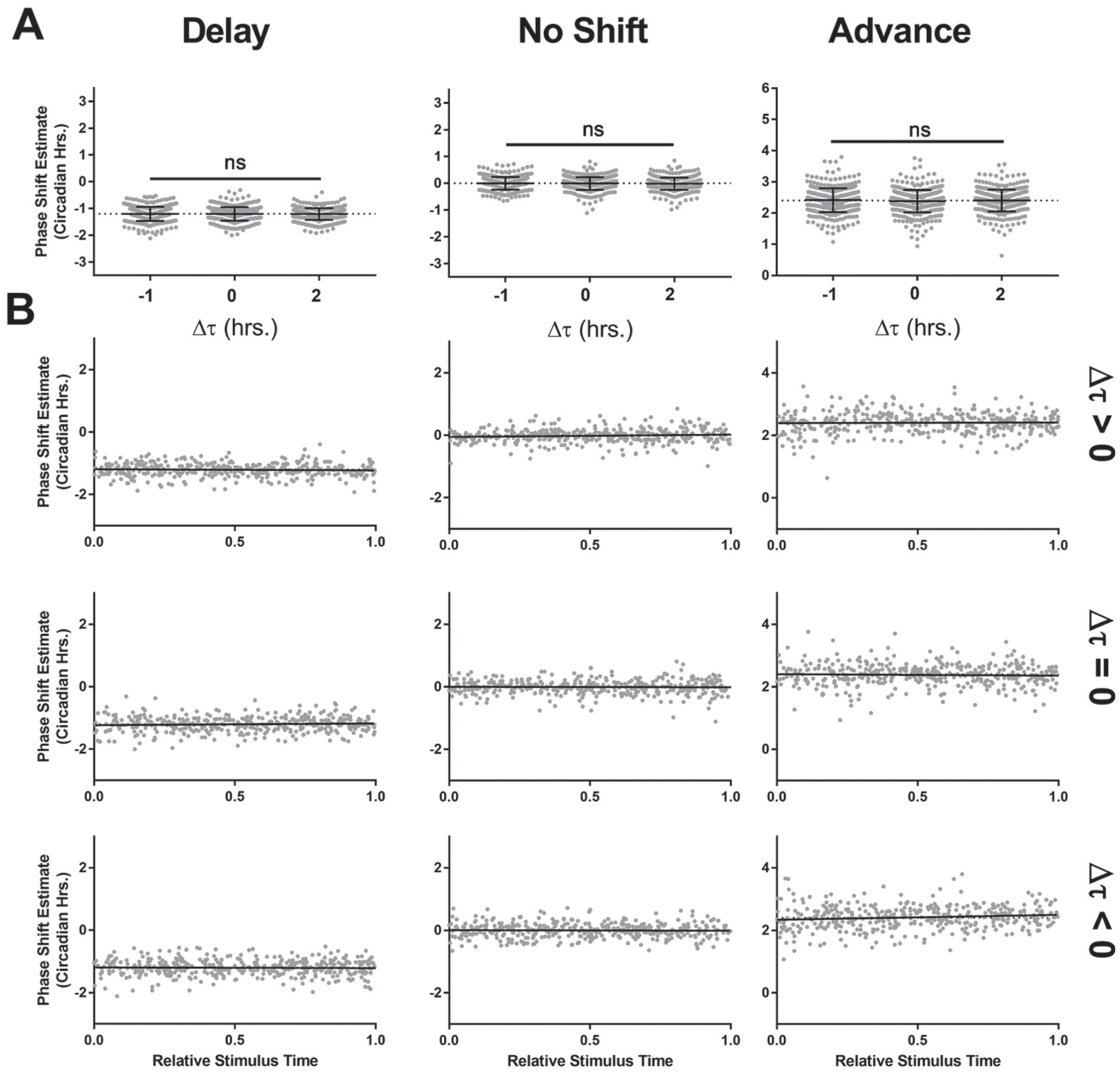
TIPA eliminates the effect of period changes and stimulus time on the phase shift estimate. (A) The estimate of the phase shift using TIPA is plotted against the period change for phase delays (left, Δϕ = −1.2), no phase shift (middle, Δϕ = 0), and phase advances (right, Δϕ = +2.4). One-way ANOVA: ns corresponds to p > 0.05. (B) The TIPA estimate of phase shift is independent of the relative stimulus time, across phase delays (left column, Δϕ = −1.2), phase advances (right column, Δϕ = +2.4), and no phase change (middle column, Δϕ = 0), as well as across period lengthening (top row, Δτ = +2), shortening (bottom row, Δτ = −1), and no period change (middle row, Δτ = 0). Each point represents 1 simulation, and each black line shows a linear fit of estimated phase shift vs. relative stimulus time. Δϕ values are represented in circadian hours.

Figure 8.

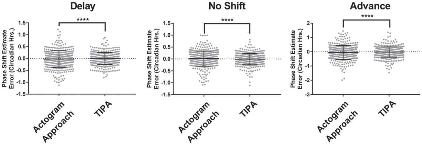
TIPA is more precise even when there is no change in period. In delay (left, Δϕ = −1.2), advance (right, Δϕ = +2.4), and no phase shift (middle Δϕ = 0) simulation groups, TIPA’s estimates of phase shift had lower variance than the actogram approach. Brown-Forsythe test for unequal variances: **** corresponds to p < 0.0001. Error bars represent standard deviation.

The actogram approach is sometimes modified for early-cycle stimulus times by anchoring the poststimulus null model to the last prestimulus phase reference point (Suppl. Fig. S4). We found that this version of the actogram approach produces a trend with a similar pattern to that of the previously described approach but with the estimate being most accurate as the relative stimulus time approaches 0 (Suppl. Fig. S4, green) rather than 1 (Suppl. Fig. S4, magenta). Using a hybrid of the two approaches, in which the phase reference point before the stimulus is used as an anchor for relative stimulus times of <0.5 and the predicted point τ_pre hours afterward is used as an anchor for relative stimulus times >0.5, results in estimates that surround the true phase shift parameter of the simulations (Suppl. Fig. S5, blue). The hybrid approach is most accurate when the stimulus time is close to either the last prestimulus phase reference point or 1 full cycle later but is less accurate when the stimulus time is between these 2 points in the cycle. Although the hybrid version improves the accuracy of the actogram approach, this accuracy is due to counteracting errors in opposite directions that only cancel each other out if relative stimulus times are evenly distributed below and above 0.5 (Suppl. Fig. S5, green, magenta). Even with this increase in accuracy, we found that the precision of TIPA significantly exceeded that of the hybrid actogram approach (Suppl. Fig. S5).

Discussion

Accurately quantifying changes in phase in circadian data sets is a critical aspect of many circadian analyses but has received less attention than quantification of period. The typical actogram approach described here is not the only strategy used to measure phase shifts, but in using linear fits of pre- and postshifted data, it is one of the only approaches that accounts for period changes (see description of cross-correlation in Dowse, 2009). Although we have used actograms as examples, the underlying strategy for measuring phase shifts using the progression of phase reference points is the same across virtually all data types and fits. As described above, the estimation of phase shifts must involve the comparison of how the pacemaker would have progressed and how it actually progressed. Making that comparison, whether by distilling full locomotor activity or gene expression rhythms down to identifiable phase reference points or by analyzing the entire wave through cosinor analysis, requires assumptions about how the pacemaker will progress after the stimulus. Previous applications of these methods are biased by assumptions regarding the change in period of the pacemaker after the stimulus. We show here that TIPA is an accurate and versatile approach to determining phase shifts in circadian data by remaining consistent across changes in period and relative time of stimulus. TIPA can be applied to any type of circadian data with multiple cycles and identifiable phase reference points, while maintaining precision throughout differing noise levels and cycle numbers.

In our study, TIPA and the actogram approach were used to estimate the phase shift in simulations, which enabled us to compare the values estimated by each method against the known phase shift parameter for that simulation group. This differs from experimental biology where the true phase shift values are unknown. TIPA, like any method designed to summarize a biological phenomenon into a single number, will have a range of error. Based upon our results, this range of error likely surrounds the true phase shift value regardless of period changes or the relative time of stimulus, in contrast to the actogram approach where the typical range of error is compounded by baseline changes dependent on those two factors. Comparing TIPA to the hybrid version of the actogram approach where the range of error surrounds the true phase shift value, TIPA’s range of error is significantly narrower.

Like all phase shift estimation methods based on phase reference points, TIPA assumes that the identified phase reference points represent the same phase of the pacemaker from cycle to cycle, even if the period of the pacemaker changes. Although this assumption is likely valid if the period changes are relatively small, it may break down as period changes become large. TIPA also assumes that the poststimulus period is stable. In many circadian experiments in which a period and/or phase change occurs, there are transient cycles poststimulus in which the rhythmic output being measured lags behind the underlying pacemaker and therefore does not reflect the pacemaker’s true phase. If applying TIPA to a dataset with transients, we recommend limiting the window of comparison to poststimulus cycles that have a stable period.

Finally, TIPA assumes that any potential phase and period changes occur nearly instantaneously. While there is experimental evidence to support the instantaneous resetting of the pacemaker’s phase (Shigeyoshi et al., 1997), the assumption that period changes occur instantaneously has not been conclusively verified. The concept of an instantaneously changed period serves as an improvement over other methods, however, which ignore the specific timing of the period change by bluntly anchoring period changes to phase reference points. This anchoring leads to inconsistent poststimulus modeling (see Fig. 4).

While many aspects of circadian data collection vary (e.g., number of cycles, sampling resolution, signal-to-noise level), the strategy of estimating phase shifts by comparing prestimulus and poststimulus models remains the same. Our results suggest that provided the data have a phase reference point and at least 3 cycles with a stable period, TIPA’s estimates are both accurate and precise. TIPA thus offers an opportunity for standardized and reproducible phase shift estimates across chronobiology.

Supplementary Material

Supplementary Material, Fig._S1 – Tau-independent Phase Analysis: A Novel Method for Accurately Determining Phase Shifts

Supplementary Material, Fig._S1 for Tau-independent Phase Analysis: A Novel Method for Accurately Determining Phase Shifts by Michael C. Tackenberg, Jeff R. Jones, Terry L. Page and Jacob J. Hughey in Journal of Biological Rhythms

Supplementary Material

Supplementary Material, Fig._S2 – Tau-independent Phase Analysis: A Novel Method for Accurately Determining Phase Shifts

Supplementary Material, Fig._S2 for Tau-independent Phase Analysis: A Novel Method for Accurately Determining Phase Shifts by Michael C. Tackenberg, Jeff R. Jones, Terry L. Page and Jacob J. Hughey in Journal of Biological Rhythms

Supplementary Material

Supplementary Material, Fig._S3 – Tau-independent Phase Analysis: A Novel Method for Accurately Determining Phase Shifts

Supplementary Material, Fig._S3 for Tau-independent Phase Analysis: A Novel Method for Accurately Determining Phase Shifts by Michael C. Tackenberg, Jeff R. Jones, Terry L. Page and Jacob J. Hughey in Journal of Biological Rhythms

Supplementary Material

Supplementary Material, Fig._S4 – Tau-independent Phase Analysis: A Novel Method for Accurately Determining Phase Shifts

Supplementary Material, Fig._S4 for Tau-independent Phase Analysis: A Novel Method for Accurately Determining Phase Shifts by Michael C. Tackenberg, Jeff R. Jones, Terry L. Page and Jacob J. Hughey in Journal of Biological Rhythms

Supplementary Material

Supplementary Material, Fig._S5 – Tau-independent Phase Analysis: A Novel Method for Accurately Determining Phase Shifts

Supplementary Material, Fig._S5 for Tau-independent Phase Analysis: A Novel Method for Accurately Determining Phase Shifts by Michael C. Tackenberg, Jeff R. Jones, Terry L. Page and Jacob J. Hughey in Journal of Biological Rhythms

Supplementary Material

Supplementary Material, TIPA_Supplementary_Figures_Revised – Tau-independent Phase Analysis: A Novel Method for Accurately Determining Phase Shifts

Supplementary Material, TIPA_Supplementary_Figures_Revised for Tau-independent Phase Analysis: A Novel Method for Accurately Determining Phase Shifts by Michael C. Tackenberg, Jeff R. Jones, Terry L. Page and Jacob J. Hughey in Journal of Biological Rhythms