Sage Journals: Discover world-class research

Abstract

A model of arousal dynamics is applied to predict objective performance and subjective sleepiness measures, including lapses and reaction time on a visual Performance Vigilance Test (vPVT), performance on a mathematical addition task (ADD), and the Karolinska Sleepiness Scale (KSS). The arousal dynamics model is comprised of a physiologically based flip-flop switch between the wake- and sleep-active neuronal populations and a dynamic circadian oscillator, thus allowing prediction of sleep propensity. Published group-level experimental constant routine (CR) and forced desynchrony (FD) data are used to calibrate the model to predict performance and sleepiness. Only the studies using dim light (<15 lux) during alertness measurements and controlling for sleep and entrainment before the start of the protocol are selected for modeling. This is done to avoid the direct alerting effects of light and effects of prior sleep debt and circadian misalignment on the data. The results show that linear combination of circadian and homeostatic drives is sufficient to predict dynamics of a variety of sleepiness and performance measures during CR and FD protocols, with sleep-wake cycles ranging from 20 to 42.85 h and a 2:1 wake-to-sleep ratio. New metrics relating model outputs to performance and sleepiness data are developed and tested against group average outcomes from 7 (vPVT lapses), 5 (ADD), and 8 (KSS) experimental protocols, showing good quantitative and qualitative agreement with the data (root mean squared error of 0.38, 0.19, and 0.35, respectively). The weights of the homeostatic and circadian effects are found to be different between the measures, with KSS having stronger homeostatic influence compared with the objective measures of performance. Using FD data in addition to CR data allows us to challenge the model in conditions of both acute sleep deprivation and structured circadian misalignment, ensuring that the role of the circadian and homeostatic drives in performance is properly captured.

Keywords

performance sleepiness alertness circadian homeostatic model prediction

In the modern 24/7 society, reduced alertness due to irregular work hours and insufficient sleep has become a major safety and productivity issue in occupational settings, on the roads, and for general health and well-being (Rajaratnam et al., 2013; Rajaratnam and Arendt, 2001). A physically based mathematical model that could predict alertness in wide variety of complicated operational settings would be of high practical utility. Alertness is affected by multiple physiological and environmental factors, including prior sleep history, chronic and acute sleep restriction, circadian phase, light exposure, use of stimulants and sedatives, work schedules, and the task being performed. So far, none of the existing models account for the complex interaction among these factors. In this study we enable prediction of most commonly used subjective sleepiness and objective performance measures in our arousal dynamics model and lay the groundwork for incorporation of these various additional factors.

Multiple models have been developed to predict alertness, sleepiness, and performance (Achermann and Borbély, 1994; Akerstedt et al., 2008; Akerstedt and Folkard, 1995, 1997; Belyavin and Spencer, 2004; Borbély, 1982; Daan et al., 1984; Folkard et al., 1999; Fulcher et al., 2010; Hursh et al., 2004; Ingre et al., 2014; Jewett and Kronauer, 1999; Johnson et al., 2004; McCauley et al., 2013; Phillips et al., 2017; Rajdev et al., 2013; Ratcliff and Van Dongen, 2011; St. Hilaire et al., 2017). Collectively, these models have been applied to predict group-level subjective sleepiness and objective performance during acute sleep deprivation, chronic sleep restriction, jet-lag, and some types of shiftwork. Despite these advances, there are several limitations: Most of the above models (1) focused on only one experimentally observed measure of alertness, which limits future testing to studies reporting that measure, and (2) used data sets with high illuminance of different levels (often >150 lux) to fit alertness parameters but did not correct for those differences. The use of experimental data obtained under different light conditions is undesirable for model development because light has been shown to directly increase alertness independent of its phase-shifting effects (Cajochen et al., 2000; Chang et al., 2013; Phipps-Nelson et al., 2003; Rahman et al., 2014; Rüger et al., 2006); thus, light must be controlled during alertness measurements if models are to be correctly calibrated.

In this study we apply our model of arousal dynamics that accounts for sleep propensity (Postnova et al., 2016) to predict sleepiness and performance and to account for the above limitations. In particular, (1) our arousal dynamics model predicts sleep times as calibrated and tested against laboratory sleep deprivation and forced desynchrony data and does not require them as an input; (2) we develop and test a variety of alertness measures against 10 published experimental studies reporting sleepiness as well as performance during controlled constant routine (CR) and forced desynchrony (FD) protocols; and (3) we select only studies that use dim light exposure (<15 lux) during wakefulness to avoid the direct alerting effects of light. We focus on FD and CR data, because FD data allow us to investigate the effects of the circadian and homeostatic drives separately on performance and sleepiness, whereas CR data demonstrate their combined effect at one particular phase relationship (Lockley et al., 2008).

Methods

A schematic of our model of arousal dynamics is shown in Figure 1. It incorporates mutually inhibitory interactions between the monoaminergic (MA) wake-active neuronal populations and the sleep-active ventrolateral preoptic nucleus (VLPO) (Phillips and Robinson, 2007; Saper et al., 2010). Activity of these populations is regulated by the homeostatic (H) and circadian (C) drives, which collectively introduce a sleep drive to the VLPO depending on the time awake and circadian phase. The phase of the drive C, in turn, depends on the prior light exposure according to the human phase- and dose-response curves (Forger et al., 1999; Jewett and Kronauer, 1999; Kronauer et al., 1999; St. Hilaire et al., 2007, 2012). The model has been used previously to examine the effects of shiftwork, sleep deprivation, caffeine, and other conditions (Fulcher et al., 2010; Phillips et al., 2011; Postnova et al., 2012, 2013; Puckeridge et al., 2011; Robinson et al., 2015) and was recently improved to account for the circadian profile of sleep propensity (Postnova et al., 2016). The model and methods for simulation of experimental protocols have been described previously in great detail (Phillips et al., 2011; Postnova et al., 2014, 2016) but we provide all equations and parameter values in Table 1 for completeness.

Figure 1.

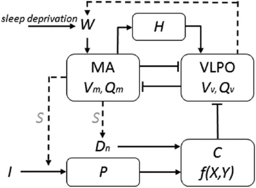
Schematic of the key model components. Illuminance of the environmental light, I, is gated by the sleep-wake state, S, and processed by the photic drive, P, which simulates the activation-deactivation dynamics of photoreceptors in the eye. Nonphotic drive, D_n, is modulated by S and, together with P, affects the circadian drive, C, which is represented by a nonlinear combination of the circadian variables X and Y. Drive C suppresses the activity of the sleep-active neurons in the ventrolateral preoptic nucleus (VLPO), reducing its mean voltage V_v and mean firing rate Q_v. The VLPO has a mutually inhibitory connection with the wake-active monoaminergic nuclei (MA), thus constituting the so-called sleep-wake switch. Activation of the MA (wake) leads to increase of the homeostatic drive H, which together with the drive C provides for a total sleep drive to the VLPO, which controls the switch between the arousal states. When sleep deprivation is simulated, a wake effort, W, is introduced to keep MA in a wake state with V_m ≥ V_WE. For further detail, see Table 1 and Postnova et al. (2016).

Table 1.

Model equations and parameter values.

Equations	Parameter Values
Differential Equations Mean voltages, V_v and V_m of the VLPO and MA $τ_{v} \frac{d V_{v}}{d t} = ν_{v m} Q_{m} - V_{v} + D_{v} (1)$ $τ_{m} \frac{d V_{m}}{d t} = ν_{m v} Q_{v} - V_{m} + D_{m} + W (2)$ Homeostatic drive $τ_{H} \frac{d H}{d t} = ν_{H m} Q_{m} - H (3)$ Circadian variables $τ_{X} \frac{d X}{d t} = Y + γ (\frac{1}{3} X + \frac{4}{3} X^{3} - \frac{256}{105} X^{7}) + ν_{X p} D_{p} + ν_{X n} D_{n} (4)$ $τ_{Y} \frac{d Y}{d t} = D_{p} (ν_{Y Y} Y - ν_{Y X} X) - {(\frac{δ}{τ_{c}})}^{2} X (5)$ Photoreceptor activity $\frac{d P}{d t} = α (1 - P) - β P (6)$	Time constants $τ_{v} = τ_{m} = 50 s;$ $τ_{H} = 59 \times 3600 s;$ $τ_{X} = τ_{Y} = 24 \times 3600 / 2 π s;$ $τ_{C} = 24.2 \times 3600 s;$ Coupling strengths $ν_{v m} = - 2.1 mV;$ $ν_{m v} = - 1.8 mV;$ $ν_{H m} = 4.57 s;$ $ν_{X p} = 37 \times 60 s;$ $ν_{X n} = 0.032;$ $ν_{Y Y} = 1 / 3 ν_{X p} s;$ $ν_{Y X} = 0.55 ν_{X p} s;$ $ν_{v H} = 1;$ $ν_{v C} = - 0.5 mV;$ External neuronal drives $A_{v} = - 10.3 mV$ ; $D_{m} = A_{m} = 1.3 mV$ ; Circadian $γ = 0.13;$ $δ = 24 \times 3600 / 0.99729 s;$ $β = 0.007 / 60 s^{- 1};$ Nonphotic drive $r = 10;$ Photic drive $ϵ = 0.4;$ $I_{0} = 100 lx;$ $I_{1} = 9500 lx;$ $α_{0} = 0.1 / 60 s^{- 1};$ Firing rate $Q_{m a x} = 100 s^{- 1}$ ; $θ = 10 mV;$ $σ^{'} = 3 mV;$ Wake effort $V_{W E} = - 0.07 mV;$ $V_{t h} = - 2 mV;$ $F_{W} = 1$ if forced wake and 0 otherwise Circadian phase MELpeak $t_{0} = 0.7 \times 3600 s$ ; CBTmin $t_{0} = 2.7 \times 3600 s$ ;
Complementary Functions Mean population firing rate $Q_{i} = \frac{Q_{\max}}{1 + \exp ([θ - V_{i}] / σ^{'})}, i = v, m (7)$ Wake effort $W = F_{W} \max {0, V_{W E} - ν_{m v} Q_{v} - D_{m}}$ (8) Total sleep drive $D_{v} = ν_{v H} H + ν_{v C} C + A_{v} (9)$ Circadian drive, sleep propensity model (Postnova et al., 2016) $C = 0.1 (\frac{1 + X}{2}) + {(\frac{3.1 X - 2.5 Y + 4.2}{3.7 (X + 2)})}^{2} (10)$ Nonphotic drive to the circadian $D_{n} = (S - \frac{2}{3}) [1 - \tanh (r X)] (11)$ Photic drive to the circadian $D_{p} = α (1 - P) (1 - ε X) (1 - ε Y) (12)$ $α = α_{0} \frac{I}{I + I_{1}} \sqrt{\frac{I}{I_{0}}} (13)$ $I = I S (14)$ State function $S = {\begin{matrix} 1, V_{m} > V_{t h} (w a k e) \\ 0, V_{m} \leq V_{t h} (s l e e p) \end{matrix} (15)$
Circadian Phase Calculation $t_{c r i t} = t_{φ c r i t} + t_{0} (16)$ $φ_{c r i t} = - 2.98 = a t a n (\frac{Y}{X}) (17)$

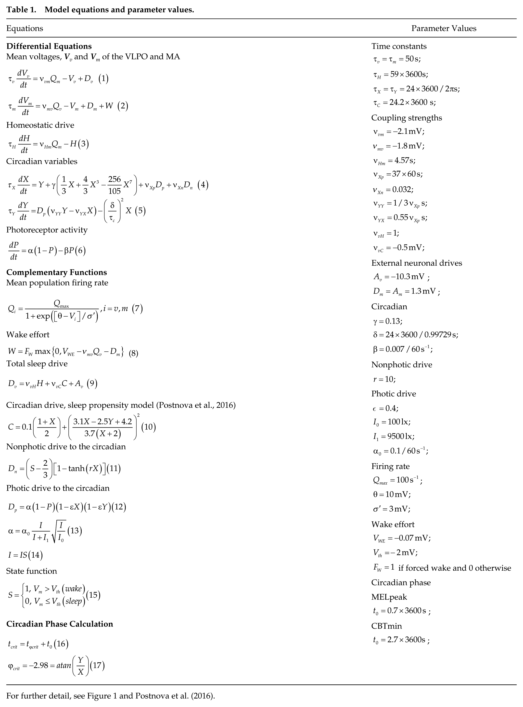
For further detail, see Figure 1 and Postnova et al. (2016).

At the start of each simulation, the model is in an entrained state with sleep appearing between 2330 and 0800 h. Ambient light conditions for entrainment are 250 lux between 0800 h and 2000 h, 40 lux outside of these hours if awake, and 0 lux during sleep.

Studies Modeled

From the experimental literature on alertness, sleepiness, and performance, we select laboratory sleep studies that described alertness dynamics in healthy participants either during acute sleep deprivation (CR) or during FD protocols and that (1) used dim light levels below 15 photopic lux during wakefulness to avoid direct alerting effects of light; (2) reported results for visual Performance Vigilance Test (vPVT) and/or Karolinska Sleepiness Scale (KSS) among other measures (vPVT and KSS were selected because they were most commonly reported in literature); (3) measured performance and sleepiness multiple times during wakefulness with protocol duration and sampling rate sufficient to illustrate the underlying circadian dynamics (typically <4 h step size for ≥24 h protocols); and (4) controlled for sleep and circadian entrainment via prestudy screening of sleep and measurement of the circadian phase at the baseline to reduce the potential effects of circadian misalignment and sleep debt on alertness. For FD protocols, we choose only those that had a 2:1 wake-to-sleep ratio to minimize effects of chronic sleep restriction because these are not yet incorporated into our model. We also do not include studies reporting results for different chronotypes, as this is beyond the aim of the current work. The resulting list of studies is shown in Table 2 with the corresponding objective and subjective measures of performance and sleepiness that were reported and are being predicted in this study.

Table 2.

Experimental studies used for model fitting and testing.

				vPVTRT
Study^a	vPVTL	ADD	KSS	Mean	Median	Fast 10%	Slow 10%	DSST
Constant Routine Data
Ftouni N = 10, CR_dur = 40 h			✓*
ShekletonN = 31, CR_dur = 50 h	✓*		✓*	✓*				✓*
ChuaN = 24, CR_dur = 40 h	✓*		✓*	✓*
JungN = 40, CR_dur = 40 h	✓*			✓*	✓*	✓*	✓*
Forced Desynchrony Data
SilvaN = 10, T = 20 h	✓*	✓*	✓*
LeeN = 11, T = 28 h	✓*	✓*		✓*		✓*
BurkeN = 6, T = 28 h		✓*	✓*					✓*
Wyatt 1999N = 6, T = 20 h	✓m	✓*m	✓m		✓m			✓*m
Wyatt 2004N = 16, T = 42.85 h			✓b					✓*b
GradyN = 18, T = 42.85 h	✓*	✓*b	✓b		✓*		✓*

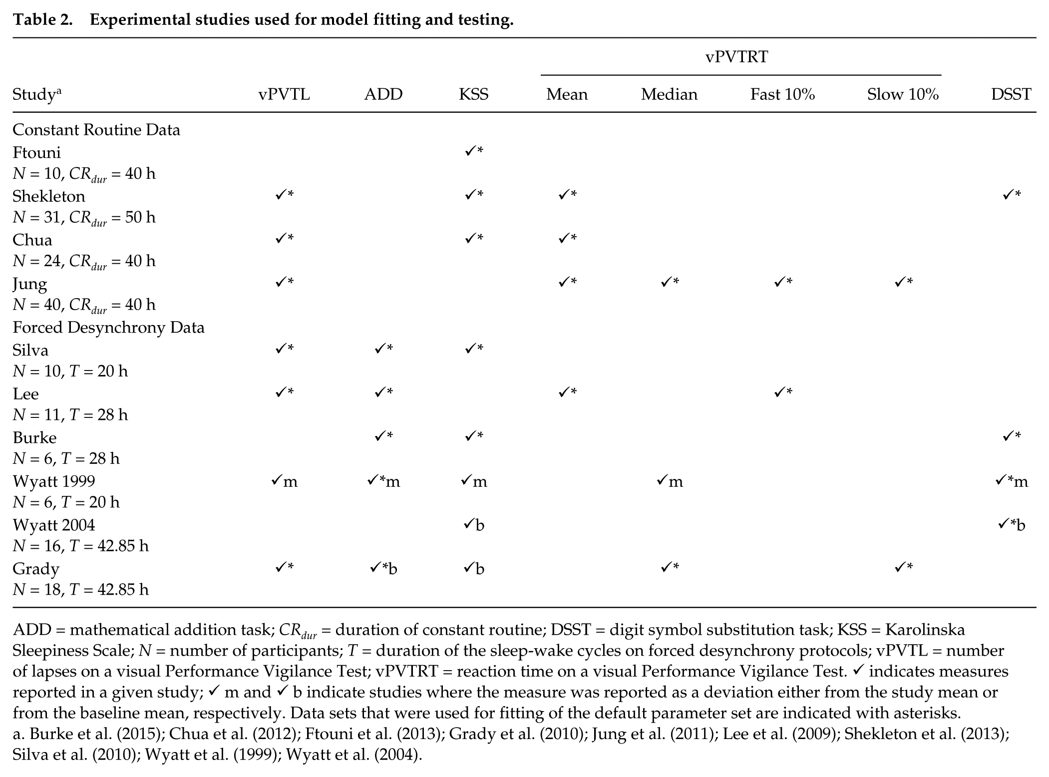
ADD = mathematical addition task; CR_dur = duration of constant routine; DSST = digit symbol substitution task; KSS = Karolinska Sleepiness Scale; N = number of participants; T = duration of the sleep-wake cycles on forced desynchrony protocols; vPVTL = number of lapses on a visual Performance Vigilance Test; vPVTRT = reaction time on a visual Performance Vigilance Test. ✓ indicates measures reported in a given study; ✓ m and ✓ b indicate studies where the measure was reported as a deviation either from the study mean or from the baseline mean, respectively. Data sets that were used for fitting of the default parameter set are indicated with asterisks.

Burke et al. (2015); Chua et al. (2012); Ftouni et al. (2013); Grady et al. (2010); Jung et al. (2011); Lee et al. (2009); Shekleton et al. (2013); Silva et al. (2010); Wyatt et al. (1999); Wyatt et al. (2004).

The CR studies in Table 2 reported dynamics over time awake in conditions of dim light and constant posture for up to 40 h of wakefulness (Chua et al., 2012; Ftouni et al., 2013; Jung et al., 2011; Shekleton et al., 2013). These reflect the interplay of the circadian and homeostatic drives in their control of sleepiness and performance at one phase relationship. Conversely, FD studies are designed to uncouple the C and H drives to study their effects separately and their interactions at all phase relationships. This is done by introducing sleep-wake cycles of durations (T) that are sufficiently different from 24 h to prevent circadian entrainment (i.e., outside the range of entrainment) and have sleep scheduled at different circadian phases. Studies considered here had T = 20 h (Silva et al., 2010; Wyatt et al., 1999), T = 28 h (Burke et al., 2015; Lee et al., 2009), and T = 42.85 h (Grady et al., 2010; Wyatt et al., 2004). These protocols lasted for about a month to collect sufficient amount of data with waking time spent in dim lighting with typical illuminance during wakefulness of 3.3 lux and never above 15 lux. Performance and sleepiness measures were collected at 1- to 3-h intervals during scheduled wake episodes.

To extract the data values from figures in publications, a java-based shareware program was used (DataThief III; http://datathief.org/). This allowed for digital estimation of data values and enabled quantitative comparison with simulated data.

Additional Processing of Experimental Data

Three measures of performance and sleepiness were most commonly reported across the above studies. (1) The first measure entailed objective measurements derived from reaction time on a visual Performance Vigilance Test (vPVTRT). All studies used a 10-min vPVT test, and the derived measurements included total number of lapses (vPVTL) during the test (a lapse is counted when vPVTRT is >500 ms), mean and median vPVTRT, and mean fastest and slowest 10% vPVTRT. (2) The second measure consisted of number of correct answers on cognitive tasks such as a mathematical addition task (ADD) and digit symbol substitution task (DSST). Duration of these tests varied across the studies from 2 to 4 min for ADD and from 1.5 to 3 min for DSST. (3) The third measure was the subjective score on the KSS, which ranges from 1 = “Extremely alert” to 9 = “Extremely sleepy, fighting sleep.”

Most experimental studies reported absolute (nonrelative) values for vPVT and KSS, with some reporting relative (e.g., to baseline or study mean) and/or otherwise transformed data. Some types of transformations, such as logarithmic transformation for vPVTRT or square root transformation for vPVTL (e.g., Anderson et al. 2013; Ftouni et al. 2013), cannot be recalculated back to absolute values from published group mean data because the transformations were done on individual data before averaging. Thus, these types of transformed data cannot be compared with nontransformed data and are not used here. We aim to predict absolute values of vPVT and KSS, so only nontransformed data are used for model calibration for these measures, while data reported as relative to baseline/study mean are used for additional testing.

Unlike vPVT and KSS, both ADD and DSST have a learning component; that is, the number of correct responses is affected not only by alertness and test duration but also by how many times the test was repeated, which varies significantly across the protocols. As a result, these data are not directly comparable between the studies. Thus, to enable comparison and modeling of ADD and DSST measures, we (1) recalculate all experimental ADD and DSST data as a mean number of correct tasks per 1 min and (2) calculate deviation from study mean, which minimizes learning effects when the data are averaged according to time after wake or to circadian phase. These processed cognitive measures, ΔADD_m and ΔDSST_m, demonstrate the overall trend of changes in performance depending on time since wake or the circadian phase but not the actual values.

Additional processing of experimental data includes removal of data that might be affected by sleep inertia, as most of the studies did not provide enough data during the first 3.5 h after awakening. Thus, sleep inertia is not modeled here, and the first 3.5 h of data are removed from all times after wake data sets to avoid the potential effects of sleep inertia on the model fitting parameters (Jewett et al., 1999).

Processing of Simulated Data

We simulate each of the experimental protocols in Table 2 with the arousal dynamics model. The outputs used to model sleepiness and performance measures are processed in the same way as reported in the respective CR and FD experiments. In particular, to align with experimental data in CR studies, values of the model variables are selected at the same times as data reported in experiments. In FD protocols for data reported versus time awake, each model variable is averaged across all wake episodes to obtain averaged time series versus time awake for that variable, and the data points at times reported in the experiments are selected. For the circadian phase dependency, the variable values observed during wakefulness are averaged within 60° circadian bins relative to core body temperature minimum (CBTmin) for all studies except Wyatt et al. (2004), where the phase is reported relative to melatonin peak (MELpeak). These processed variables are then used to predict performance and sleepiness.

Modeling Performance and Sleepiness

We use multivariate linear regression to predict temporal dynamics of performance and sleepiness measures from variables of the arousal dynamics model. A general form for linear regression is

A = Θ F = Θ_{0} + Θ_{1} F_{1} + Θ_{2} F_{2} + \dots + Θ_{n} F_{n},

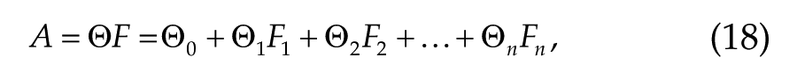
where A is the desired alertness measure, n is the number of input variables, and F is the matrix of input variables with each variable represented by a vector of values F_j. Equation 18 is directly applied for prediction of KSS and vPVT measures. Prediction of ΔADD_m and ΔDSST_m requires adjustment, however, as deviations from the study mean rather than absolute values are predicted to avoid learning effect. In this case, Equation 1 is modified as

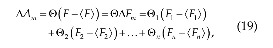
\begin{array}{l} Δ A_{m} = Θ (F - 〈 F 〉) = Θ Δ F_{m} = Θ_{1} (F_{1} - 〈 F_{1} 〉) \\ + Θ_{2} (F_{2} - 〈 F_{2} 〉) + \dots + Θ_{n} (F_{n} - 〈 F_{n} 〉), \end{array}

with m denoting deviation from the study mean. Equation 19 has one less parameter than Equation 18 because the bias term is zero.

Calibration and Resulting Default Parameter Set

To determine the default parameter set, Θ, that should be used in future predictions of performance and sleepiness where no information except a protocol is available, we calibrate the model by fitting it to all suitable data at the same time. The studies used for fitting the default parameter set for different measures are indicated with an asterisk in Table 2. The vector of parameters Θ that gives the best fit to experimental observations E is found by solving the normal equation:

Θ = {(F^{T} F)}^{- 1} F^{T} E .

For the fitting of deviations from the mean, this is represented by

Θ = {(Δ F_{m}^{T} Δ F_{m})}^{- 1} Δ F_{m}^{T} Δ E_{m} .

The same formula is used for fitting deviations from the baseline mean (b). In Table 2, the studies reporting deviation from the study and baseline means are indicated with m and b, respectively.

We use leave-one-out cross-validation to estimate how well this default model would generalize to an independent data set for each of the sleepiness and performance measures. To do so, we iteratively choose one test study for each of the modeled measures and fit the model in Equations 18 or 19 to the remaining data. The goodness of fit is then calculated for the test data using normalized root mean squared error (NRMSE):

N R M S E = \frac{\sqrt{\sum_{i = 1}^{N} {(A_{i} - E_{i})}^{2}}}{\sqrt{N} [\max (E) - \min (E)]},

where N is the number of data points. The final prediction error, 〈NRMSE〉, was calculated as the mean of the errors (NRMSE) across all test data sets. We also calculated prediction error including studies reporting data relative to mean or baseline, 〈NRMSE_mb〉. This is the same as 〈NRMSE〉 for relative measures (ΔADD_m and ΔDSST_m) but different for vPVT and KSS, because for them the relative data were not used in calibrating the default parameter set.

The goodness of fit is best when NRMSE = 0, indicating that predicted data fully coincides with experimental data (A = E). NRMSE > 1 indicates that on average, the difference between predictions and data is larger than the experimental data range. Overall, lower NRMSE indicates better agreement between the model and the data.

Results

Of the measures reported in the experimental studies in Table 2, we focus on vPVTL, ΔADD_m, and KSS, because they had the most available data. We also demonstrate default parameter sets and prediction error for the remaining measures, ΔDSST_m and vPVTRT, but note that those should be revisited when more data are available.

Since both the homeostatic and circadian drives are known to affect alertness measures, we test different homeostatic and circadian input variable combinations. The physiological mechanisms of various alertness measures are still not known. Thus, it is important to test different input combinations to (1) examine whether the same inputs can predict different outputs (e.g., both objective and subjective measures) and (2) identify the smallest number of inputs allowing for a good quantitative fit. Circadian variables include C, X, Y and W (wake effort), and the homeostatic variables are H and W. Note that the wake effort, W (not to be confused with the Process W describing sleep inertia in Akerstedt and Folkard, 1995), is affected by both H and C and thus appears in both sets. We find that (1) linear combinations with 2 input variables (one homeostatic and one circadian) demonstrate similar 〈NRMSE〉 compared with combinations with 3 or more input variables despite their having a higher number of fitting parameters; (2) use of W alone, as done by Fulcher et al. (2010), provides a good overall fit but underpredicts circadian influence during prolonged wakefulness; (3) most of the 2-variable combinations demonstrate similar prediction error but combinations H,X, and H,Y show worse overall performance with an average of 33% higher 〈NRMSE〉 across the sleepiness and performance measures; (4) the remaining five 2-variable combinations all showed good predictions with mean 〈NRMSE〉 across vPVTL, ΔADD_m, and KSS of 0.37 ± 0.06. As such, there is not enough evidence to clearly select one of these linear combinations over the other on the basis of their performance on the available data set.

We show detailed results for a linear combination of H and C, because this (1) allows us to study the ratio of the homeostatic and circadian influence on performance and sleepiness directly and (2) is commonly used in other models based on the two-process concept. Equation 18 for prediction of sleepiness/performance measures, A, is thus modified as

A = Θ_{0} + Θ_{H} H + Θ_{C} C .

Calibrated Model and Default Parameter Set

Table 3 shows the parameters Θ₀, Θ_H, Θ_C, for the different performance and sleepiness measures obtained by simultaneously fitting the linear combination of H and C produced by simulation of the experimental protocols with the arousal dynamics model to all eligible data (see Methods). These are the default parameters that should be used for prediction of performance and sleepiness when there is no prior knowledge of participants’ dynamics. The prediction errors 〈NRMSE〉 and 〈NRMSE_mb〉 in Table 3 show how well the model would be expected to perform against an independent data set as calculated with a standard leave-one-out cross-validation approach and, in case of PVT and KSS, addition of independent testing data sets reporting values relative to study and baseline mean. As seen from the table, the prediction error for ΔADD_m (〈NRMSE〉 = 0.19) is lower than for vPVTL or KSS (0.4 and 0.23). This is explained by subtraction of the study mean from the ADD values, which minimizes individuals’ inherent variation in ADD levels and learning rates, leaving only the dynamic response to the protocols. The error calculated across all available data for vPVTL and KSS including the testing data sets reported as relative to study/baseline mean 〈NRMSE_mb〉, however, indicates improved prediction for vPVTL and worsened predictions for KSS (0.38 vs. 0.4).

Table 3.

Default parameters and model prediction error.

				vPVTRT, ms
	vPVTL	ΔADD_m	KSS	Mean	Median	Fast 10%	Slow 10%	ΔDSST_m
$Θ_{0}$	−137.49 (–66.21)	—	−24.34 (22.43)	−12787 (–1768)	−1736	−4.99	−12473	—
$Θ_{H}$	11.77 (6.20)	−1.35	2.28 (2.13)	1055 (180)	168	17.77	1096	−6.29 (–5.88)
$Θ_{C}$	−12.47 (–11.13)	1.42	−1.74 (–1.74)	−1144 (–363)	−214	−18.75	−1830	6.97 (6.50)
\| $Θ_{H} / Θ_{C} \|$	0.94 (0.56)	0.95	1.30 (1.22)	0.92 (0.50)	0.79	0.95	0.60	0.90 (0.90)
$〈 N R M S E 〉$	0.40 (0.31)	0.19	0.23 (0.29)	1.48 (0.43)	0.26	0.71	0.24	0.20 (0.24)
$〈 N R M S E_{m b} 〉$	0.38 (0.30)	0.19	0.35 (0.40)	—	0.63	—	—	0.20 (0.24)

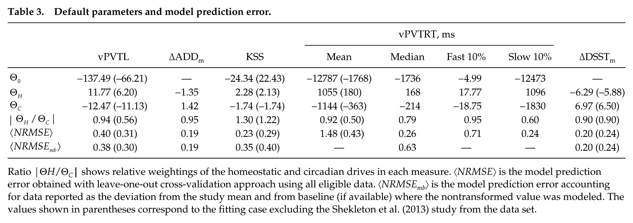
Ratio |Θ_H/Θ_C| shows relative weightings of the homeostatic and circadian drives in each measure. 〈NRMSE〉 is the model prediction error obtained with leave-one-out cross-validation approach using all eligible data. 〈NRMSE_mb〉 is the model prediction error accounting for data reported as the deviation from the study mean and from baseline (if available) where the nontransformed value was modeled. The values shown in parentheses correspond to the fitting case excluding the Shekleton et al. (2013) study from the data set.

The higher 〈NRMSE〉 for vPVTL compared with KSS is largely explained by the differences in the PVT data reported in the study by Shekleton et al. (2013) compared with the others as demonstrated in Figure 2. Conversely, KSS values reported by Shekleton et al. are similar to the other studies. The protocols and measurements in these studies are nearly identical, so the differences in vPVT are expected to be mainly due to individual variability and small numbers of subjects in all studies (n < 20). To demonstrate this, we also fit the model and run cross-validation for all studies excluding the Shekleton et al. data, which leads to a lower 〈NRMSE〉 = 0.31 for vPVTL but a slightly higher 〈NRMSE〉 = 0.28 for KSS.

Figure 2.

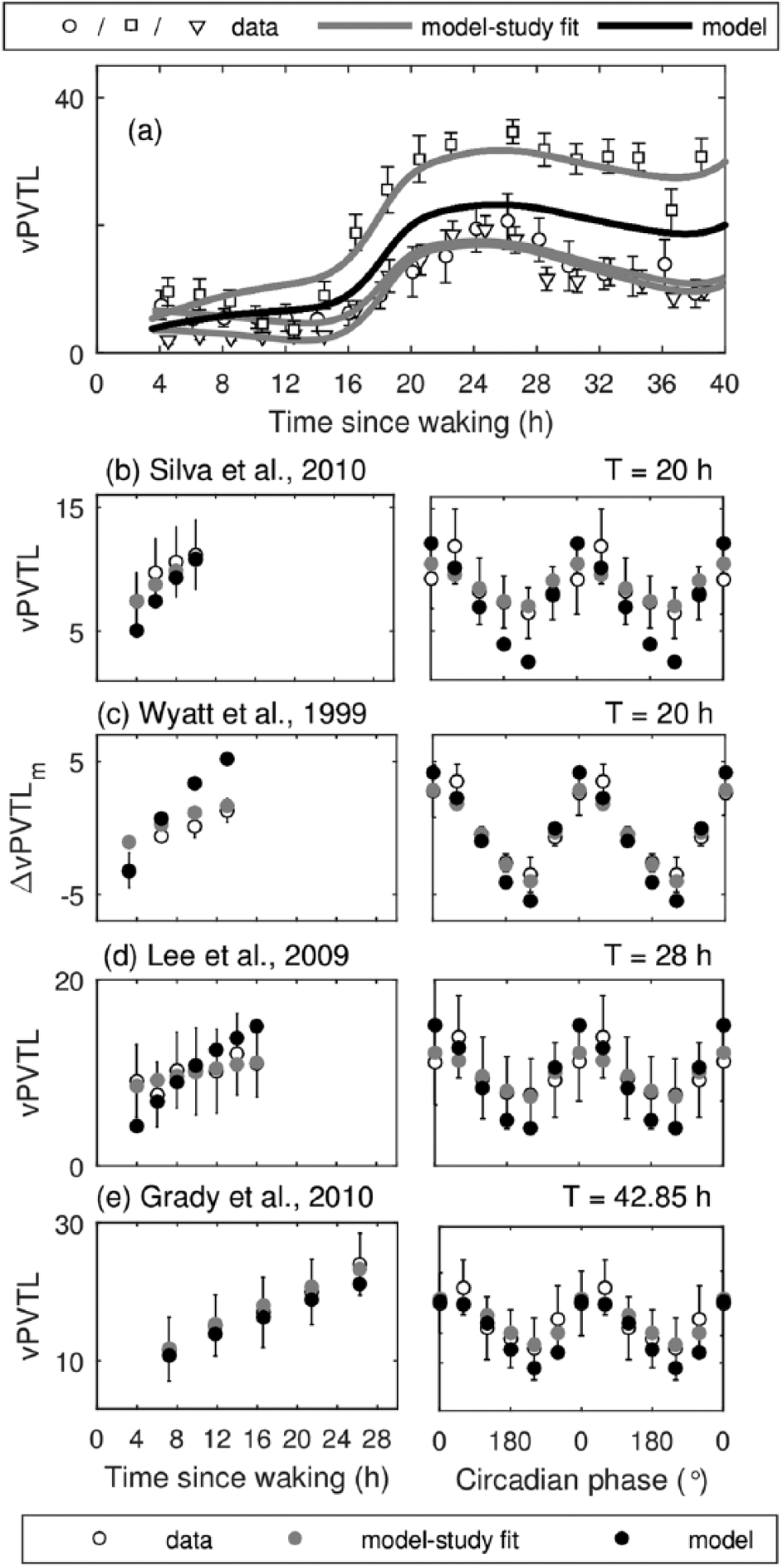
Model predictions for the number of visual PVT lapses (vPVTL) compared with experimental data obtained during constant routine (CR) and forced desynchrony (FD) protocols. Model predictions with nominal data set are shown with solid black line for CR and filled black circles for FD protocols. Best model fits to individual studies are shown in gray and data are shown with open symbols. (a) vPVTL versus time awake during CR. Experimental data are from Jung et al. (2011) (○), Shekleton et al. (2013) (□), and Chua et al. (2012) (∇). (b) vPVTL dynamics on T = 20 h protocol by Silva et al. (2010). (c) dynamics of vPVTL relative to study mean on T = 20 h protocol by Wyatt et al. (1999). (d) vPVTL dynamics on T = 28 h protocol by Lee et al. (2009) and (e) on T = 42.85 h protocol by Grady et al. (2010). Left panels show data versus time awake. Right panels show data versus circadian phase relative to CBT minimum, which are averaged within 60° circadian bins.

To estimate how good the obtained 〈NRMSE〉 values are, we also calculate NRMSE between experimental studies to estimate variability in experimental data. We find that NRMSE comparing experimental data on similar protocols ranges from 0.103 for ΔADD_m to 0.87 for vPVTL and 0.419 for KSS. This shows that our model prediction error falls in the range of between-study variability.

The goodness of fit obtained with the default parameter set for the specific studies is shown in Table 4 and the dynamics are shown in Figures 2 through 4. In addition, we demonstrate the dynamics and goodness of fit for best fits to individual studies, where Equation 6 is fitted to each data set separately, to examine variability in fitted parameters among the studies in Figure 5 and compare to the default model.

Table 4.

Goodness of fit for default parameters compared with best study fit in specific studies.

Measure	Study^a	Constant Routine		Forced Desynchrony
		Constant Routine		Time Since Waking		Circadian Phase
		NRMSE Default	NRMSE Study Fit	NRMSE Default	NRMSE Study Fit	NRMSE Default	NRMSE Study Fit
vPVTL	Shekleton	0.23	0.11	—	—	—	—
	Chua	0.37	0.09	—	—	—	—
	Jung	0.35	0.10	—	—	—	—
	Silva	—	—	0.48	0.17	0.49	0.22
	Lee	—	—	0.62	0.18	0.45	0.18
	Grady	—	—	0.13	0.07	0.27	0.16
ΔvPVTL_m	Wyatt 1999	—	—	0.58	0.28	0.19	0.10
ΔADD_m	Silva	—	—	—	—	0.21	0.10
	Burke	—	—	0.14	0.14	0.14	0.14
	Lee	—	—	0.35	0.20	0.14	0.15
	Wyatt 1999	—	—	0.28	0.24	0.19	0.16
	Grady	—	—	0.11	0.08	0.21	0.20
KSS	Ftouni	0.14	0.08	—	—	—	—
	Shekleton	0.09	0.08	—	—	—	—
	Chua	0.21	0.12	—	—	—	—
	Silva	—	—	1.4	0.24	0.14	0.09
	Burke	—	—	0.42	0.17	0.53	0.23
ΔKSS_b	Wyatt 2004	—	—	0.97	0.29	1.77	0.15
ΔKSS_b	Grady	—	—	0.48	0.15	0.62	0.12
ΔKSS_m	Wyatt 1999	—	—	1.10	0.29	0.13	0.10
vPVTRT	Shekleton	0.21	0.12	—	—	—	—
	Chua	2.74	0.11	—	—	—	—
	Jung	0.66	0.15	—	—	—	—
	Lee	—	—	2.3	0.23	1.07	0.26
vPVTRT, median	Jung	0.22	0.22	—	—	—	—
vPVTRT, median	Grady	—	—	0.21	0.20	0.30	0.30
ΔvPVTRT_m, median	Wyatt 1999	—	—	2.25	0.25	1.40	0.08
vPVTRT, fast 10%	Jung	0.20	0.09	—	—	—	—
vPVTRT, fast 10%	Lee	—	—	1.09	0.20	0.36	0.10
vPVTRT, slow 10%	Jung	0.15	0.14	—	—	—	—
vPVTRT, slow 10%	Grady	—	—	0.18	0.16	0.27	0.20
ΔDSST_m	Shekleton	0.13	0.12	—	—	—	—
	Burke	—	—	0.18	0.18	0.15	0.12
	Wyatt 2004	—	—	0.17	0.14	0.15	0.12
	Wyatt 1999	—	—	1.21	0.32	0.31	0.12

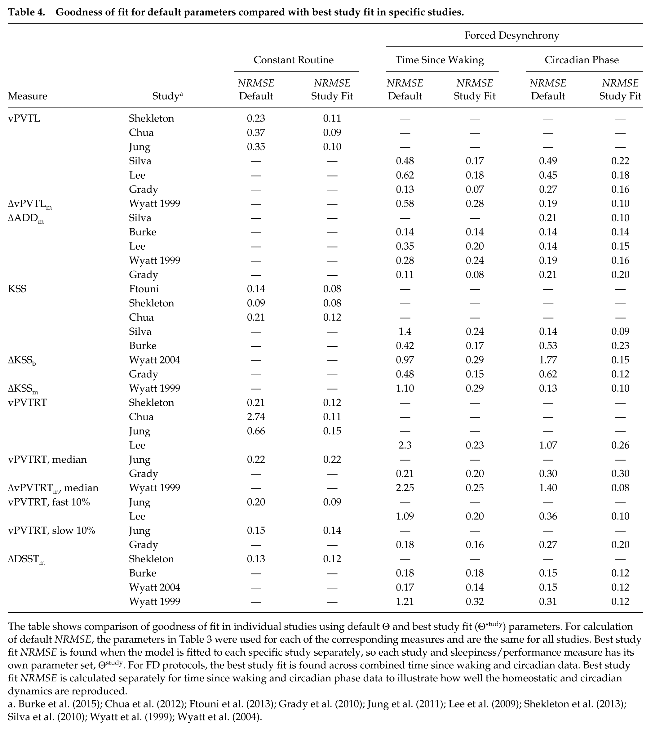
The table shows comparison of goodness of fit in individual studies using default Θ and best study fit (Θ^study) parameters. For calculation of default NRMSE, the parameters in Table 3 were used for each of the corresponding measures and are the same for all studies. Best study fit NRMSE is found when the model is fitted to each specific study separately, so each study and sleepiness/performance measure has its own parameter set, Θ^study. For FD protocols, the best study fit is found across combined time since waking and circadian data. Best study fit NRMSE is calculated separately for time since waking and circadian phase data to illustrate how well the homeostatic and circadian dynamics are reproduced.

Prediction of Objective Performance—vPVTL

Comparison of the model dynamics with experimental data for vPVTL is shown in Figure 2, with the goodness of fit to specific studies reported in Table 4. For vPVTL, the default parameter set Θ₀, Θ_H, Θ_C in Table 3 is calibrated by fitting to data from 3 CR and 3 FD studies shown in Figure 2 (a, b, d, e). The FD study by Wyatt et al. (1999) in Figure 2c is used only for testing because it reported values relative to study mean. We demonstrate the dynamics of the default model (shown in black) along with the best study fit (gray) obtained by fitting to the specific studies separately.

On a CR protocol in Figure 2a, the default model (black line) predicts vPVTL dynamics that fall between the experimentally reported values due to large variability in the experimental data. The high number of lapses reported in the study by Shekleton et al. compared with others leads to increased homeostatic influence in the default parameter set. Individual study fits, however, show very good qualitative and quantitative agreement with all three CR data sets. A low number of lapses is observed during the first 16 h after awakening, and the wake maintenance zone (WMZ) is prominent in the individual fits for studies by Chua et al. (2012) and Jung et al. (2011). The worst vPVTL performance (23 lapses) on the protocol is observed at 24.5 to 27 h after awakening (~0830-1130 h). The performance subsequently improves as time awake is increased due to circadian influence and reaches 19 lapses at 37.8 h after waking (~2150 h).

The model simulations of the FD protocols in Figure 2 (b-e) reproduced the decrease in performance (increase in vPVTL) as a function of time since wake with the default parameter set providing good agreement across 2 out of 4 studies. The best study fit parameters allow for near identical match to most data with mean NRMSE of 0.17, demonstrating that the observed difference for the default set is likely due to individual variability between studies participants.

The model, likewise, reproduces the dynamics versus circadian phase with maximum vPVTL (worst performance) predicted at CBTmin (0° or 0600 h) and minimum at 240 circadian degrees (2200 h). Interestingly, most of the experimental studies show slightly higher vPVTL at 60° (1000 h) than at 0°. However, due to averaging of the experimental data over 4-h intervals (60° bins) the exact position of the maximum and minimum of performance in the data cannot be estimated. The observed difference in the position of vPVTL maximum in the model and data in Figure 2 (b-e) can be related to differences in timing of CBTmin because the data are plotted relative to CBTmin. In the model, timing of CBTmin is adjusted based on Dijk et al. (1997) (see Postnova et al., 2016) and, thus, appears at 0600 h. In the experimental studies considered here, CBTmin was not reported, so it can be different from that used in the model.

Prediction of Objective Performance with Learning Effect—ΔADD_m

Predictions for ADD deviations from the study mean (i.e., number of correct answers on mathematical tasks per minute relative to study mean) are shown in Figure 3 and demonstrate very good agreement with experimental studies for both default and best study fit cases, as confirmed by low NRMSE in Table 4. Here the default parameter set was calibrated using all available data because we predict ADD relative to study mean rather than actual values (due to learning effect).

Figure 3.

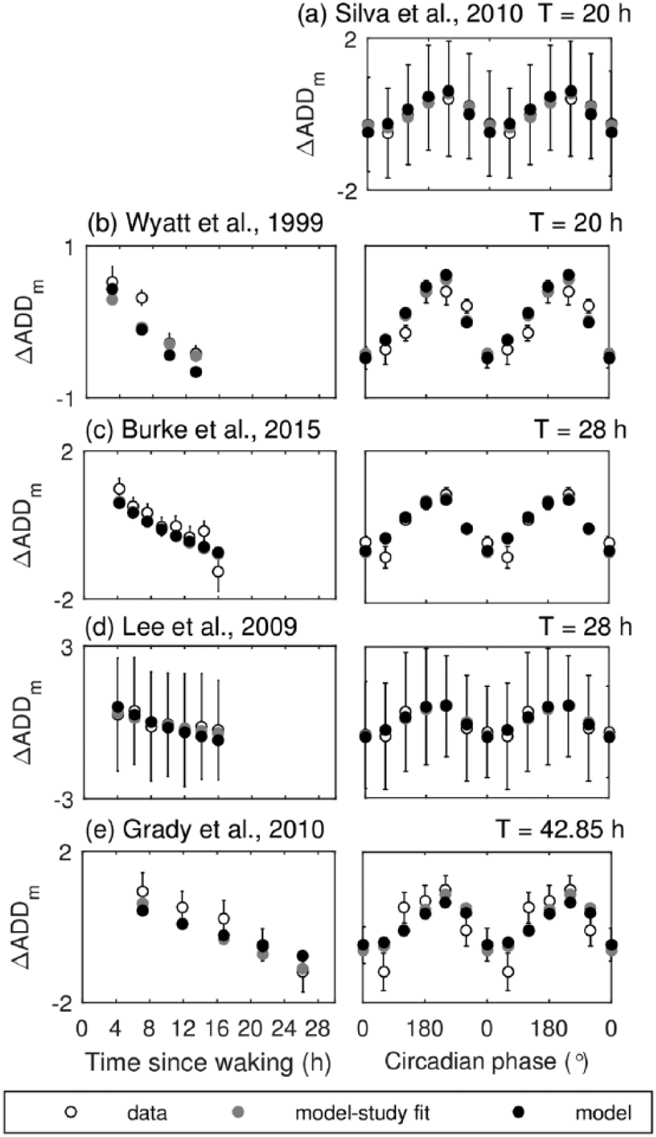
Model predictions for number of correct ADD tasks per minute relative to the protocol mean versus experimental data on FD protocols. Model predictions with the default parameters are shown with filled black circles, best fit to individual studies are shown with filled gray circles, and data are shown with open circles. In all simulations, left panels show data versus time awake. Right panels show data versus circadian phase relative to CBT minimum, which are averaged within 60° circadian bins. (a) Dynamics of ADD per minute relative to study mean on T = 20 h protocol by Silva et al. (2010) (the only circadian data available); (b) on T = 20 h protocol by Wyatt et al. (1999); (c) on T = 28 h protocol by Burke et al. (2015); (d) on T = 28 h protocol by Lee et al. (2009); (e) on T = 42.85 h protocol by Grady et al. (2010).

As expected, ΔADD_m performance decreases with time awake on all FD protocols. Dependence on circadian phase in the right panels of Figure 3 shows a profile similar to those of vPVTL, with best performance at 240° (2200 h in the entrained case) and worst around 0°. Notably, the worst ADD performance in the experimental data has been reported at both 0° (Fig. 3b) and 60° (Fig. 3, c and e), with some studies demonstrating similar values at these circadian phases (Fig. 3, a and d).

Overall, quantitative agreement for ΔADD_m is better than for other measures as demonstrated with low NRMSE in Table 4 and explained above for the default parameter set. This is further confirmed by nearly identical predictions for default and best study fit parameter sets (the gray markers in Fig. 3 mostly overlap with the black ones).

Prediction of Subjective Sleepiness—KSS

Comparison of the model KSS dynamics with experimental data is shown in Figure 4 for both CR (Fig. 4a) and FD (Fig. 4, b-f) protocols with the quantitative goodness of fit to specific studies in Table 4. The default parameters were identified using 2 CR and 2 FD studies (Fig. 4, a, b, d). The studies in Figure 4 (c, e, and f) were used only for testing as they report KSS relative to study (n = 1) and baseline (n = 2) mean.

Figure 4.

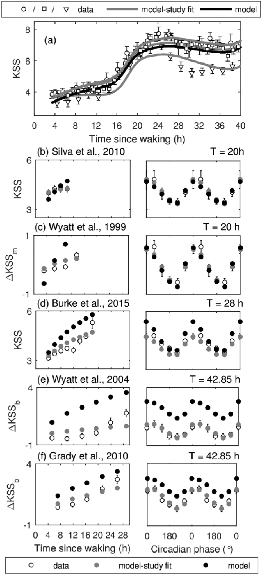
Model predictions for KSS compared with experimental data obtained during constant routine (CR) and forced desynchrony (FD) protocols. Model predictions with the default parameters are shown with solid black line for CR and filled black circles for FD. Best model fits to individual studies are shown in gray, and data are shown with open symbols. (a) Predicted and experimental KSS versus time since wake during CR. Experimental data are from Ftouni et al. (2013) (○), Shekleton et al. (2013) (□), and Chua et al. (2012) (∇). (b) KSS dynamics on T = 20 h protocol by Silva et al. (2010); (c) dynamics of KSS relative to study mean on T = 20 h protocol by Wyatt et al. (1999); (d) KSS dynamics on T = 28 h protocol by Burke et al. (2015); (e) dynamics of KSS relative to baseline mean on T = 42.85 h protocol by Wyatt et al. (2004); and (f) KSS relative to baseline mean on T = 42.85 h protocol by Grady et al. (2010). Right panels show data versus circadian phase relative to melatonin peak in Figure 4e and to CBT minimum otherwise.

In the CR case (Fig. 4a), the model predicts a gradual increase of KSS (increased sleepiness) during normal wake without the WMZ in any of the predictions, which is consistent with experimental observations. KSS increases abruptly after about 16 h of wakefulness (2400 h with 0800 h wake time) and reaches highest sleepiness on the protocol (KSS = 6.9) at 26.1 h after awakening (i.e., around 1000 h). Sleepiness decreases afterward due to circadian influence and reaches a local minimum around 36.5 h after awakening (~2030 h). The key features of KSS dynamics are also reproduced in FD protocols in Figure 4 (b-f). KSS increases with time awake, in qualitative agreement with the data as seen in the left panels. When plotted against the circadian phase (right panels), KSS shows circadian variation with minimum sleepiness at 240° (2000 h) relative to CBTmin and maximum sleepiness at 0° (0600 h).

As seen from the low NRMSE values in Table 4 and Figure 4, the model shows good agreement with CR and most of the FD studies. However, the default model prediction for ΔKSS_b for FD data in Wyatt et al. (2004) (Fig. 4d) and Grady et al. (2010) (Fig. 4e) shows a systematic error with the model predictions shifted to higher values, indicating the likely lower baseline KSS levels in the model compared with both data sets. Notably, the results in the two experiments do not align well with each other either (NRMSE between these studies is 0.419) demonstrating systematically higher values in the study by Grady et al. (2010) (by ~1 KSS point) despite its identical protocol to Wyatt et al. (2004). Individual fits to these studies, however, show very good alignment with the data as seen by significantly lower NRMSE in Table 4, indicating that the observed differences are likely due to individual variability and not due to differences in the underlying mechanisms.

Parameter Scatter in Individual Studies

Fitting the model to individual studies, as done above for the best study fits, allows us to investigate variability of the fitting parameters across these studies. Such variability is expected due to interindividual variability, which affects group averages reported in the papers, especially when the number of subjects is small, which is the case for most CR and FD experiments.

Figure 5 demonstrates the variability in parameter pairs of $Θ_{H}^{study}$ and $Θ_{C}^{study}$ obtained when the model is fitted to specific studies for vPVTL, ΔADD_m, and KSS. The study ratios of the homeostatic to circadian weights for specific measures, $| Θ_{H}^{s t u d y} / Θ_{C}^{study} |$ , vary from 0.47 to 1.43 with a mean of 0.85 for vPVTL (Fig. 5a); from 0.6 to 1.07 with a mean of 0.88 for ΔADD_m (Fig. 5b); and from 0.29 to 1.30 with a mean of 0.78 for KSS (Fig. 5c). The parameter pairs are scattered around the |Θ_H| = |Θ_C| line with the majority falling below it, thus predicting a slightly stronger effect of the model circadian drive than the homeostatic drive on the measures of sleepiness and performance in specific studies. The model with the default parameter set, however, does not reflect the same dynamics and predicts stronger homeostatic effects for KSS than for vPVTL and ΔADD_m, as shown with triangles in Figure 5 and quantified in Table 3 (|Θ_H/Θ_C|_KSS = 1.3, |Θ_H/Θ_C|_vPVTL = 0.94). Similar fitting of individual rather than group average data may provide further insight into the effects of homeostatic and circadian drives on different measures. Notably, the individual fit parameters for the Shekleton et al. study are positioned distinctly away from the other studies, demonstrating higher absolute values for both $Θ_{H}^{study}$ and $Θ_{C}^{study}$ .

Figure 5.

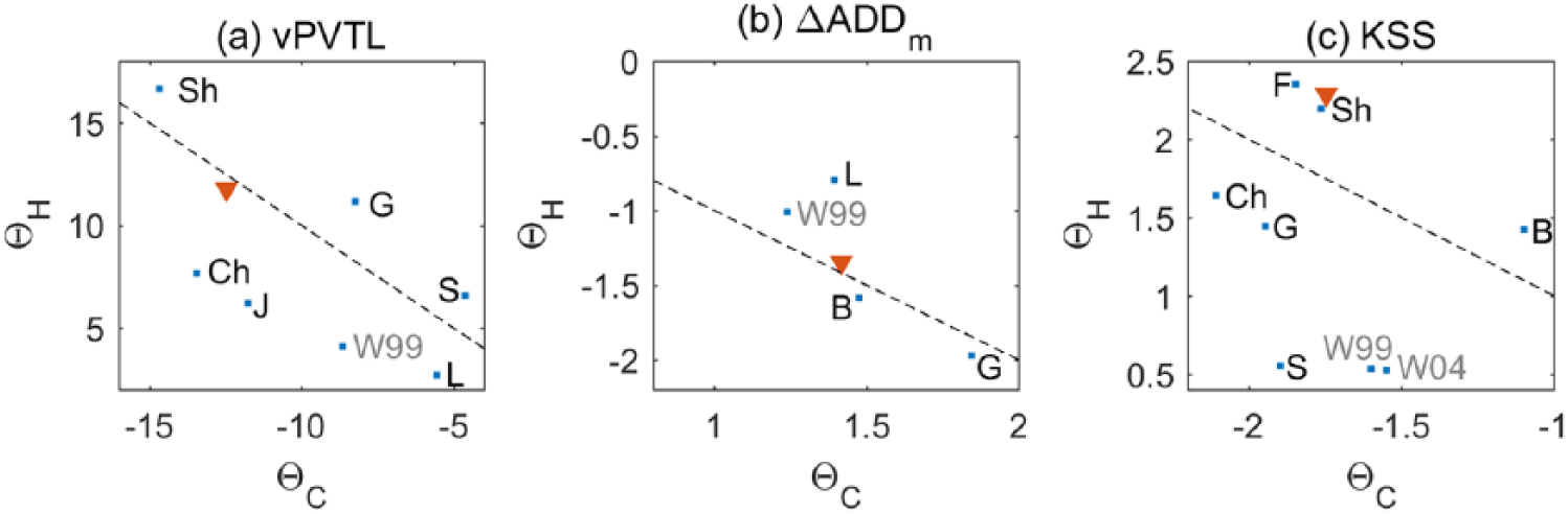
Scatter plots of best study fit parameters. (a) Best Θ^study fits for studies reporting visual performance lapses, vPVTL; (b) best Θ^study fits for ΔADD_m; and (c) best Θ^study fits for KSS. Pairs of parameters $Θ_{H}^{study}$ and $Θ_{C}^{study}$ for which the best fit is obtained for a given study are indicated with black dot and a letter referring to the study: B = Burke et al. (2015); Ch = Chua et al. (2012); F = Ftouni et al. (2013); G = Grady et al. (2010); J = Jung et al. (2011); L = Lee et al. (2009); S = Silva et al. (2010); Sh = Shekleton et al. (2013); W99 = Wyatt et al. (1999); W04 = Wyatt et al. (2004). Default parameters of the model calibrated on all eligible data are shown with filled triangles. Studies that were not used in fitting the nominal parameter set are indicated in gray. Dashed line shows a line of equal weights of H and C (i.e., |Θ_H/Θ_C| = 1).

Discussion

We demonstrated application of our arousal dynamics model to predict objective performance and subjective sleepiness during acute sleep deprivation and structured circadian misalignment. We have calibrated the model for dynamic prediction of widely used experimental measures: lapses on a visual performance vigilance test (vPVTL), correct additions on a mathematical addition task (ADD), and a subjective sleepiness score on the Karolinska Sleepiness Scale (KSS). We have also determined initial estimates for the default parameter sets to predict other vPVT measures (e.g., reaction time) and performance on a digit symbol substitution task (DSST), which can be further improved when more data become available. Other measures (e.g., ocular measures of drowsiness) can now also be implemented following the steps presented here. Prediction of a variety of measures allows for a broader validation of the model against experimental studies, which was limited in prior models because they focused on one or the other of these measures.

We find that all of the considered performance and sleepiness measures can be predicted using a linear combination of the same two model variables, the homeostatic and circadian drives, which is in line with earlier studies showing strong correlation between the measures (Bermudez et al., 2016). This confirms involvement of the same core mechanisms responsible for the alertness-related dynamics on a variety of tasks, even though there are differences in the specific physiological systems involved (e.g., muscle reaction for vPVT and subjective estimates for KSS). Furthermore, we have also found that almost every 2-variable combination of the arousal dynamics model variables reflecting homeostatic (H, W) and circadian (C, X, Y, W) dynamics is able to predict sleepiness and performance measures fairly well. Prediction of sleepiness and performance measures using wake effort alone, as done by Fulcher et al. (2010), is also successful in the improved model, but the fit is better for models with two variables.

The model predicts that different measures require different ratios between the circadian and homeostatic drives (|Θ_H/Θ_C|). Based on the default parameters, the impact of the homeostatic drive is predicted to be stronger in KSS than in the objective measures as shown in Table 3. Examination of H/C contribution in specific studies, however, does not fully align with the prediction based on combined data. Instead the Θ_H, Θ_C pairs are scattered around the equity line as shown in Figure 5, so more data are needed to clarify the dependencies.

The ratio between the homeostatic and circadian drives is again different in their effect on sleep times and sleep propensity with |Θ_H/Θ_C| = 2, found to reproduce sleep latency dynamics on forced desynchrony protocols (Postnova et al., 2016). Interestingly, the original model of Phillips et al. (2010, 2011) implied |Θ_H/Θ_C| = 0.17 for sleep-wake cycles, which is significantly lower than any of the ratios obtained here or by Postnova et al. (2016) and inferred a strongly dominating circadian drive. The present findings with the model calibrated on data suggest a more balanced influence of both the circadian and homeostatic drives on alertness and sleep than found in earlier model versions.

As demonstrated with the prediction error in Table 3, the model shows good agreement with experimental data for KSS, vPVTL, and ΔADD_m obtained during constant routine protocols of up to 40 h of wakefulness and during forced desynchrony protocols with different durations of sleep-wake cycles, T = 20, 28, and 42.85 h. The default parameter set fitted across available studies allows for future predictions of mean group performance and sleepiness levels when no prior knowledge about subjects’ dynamics is available. Fitting to specific study protocols, as shown with the best study fits in Figures 2 through 4, is useful to improve predictions when alertness data are available on one protocol for a subject or group of subjects and predictions are needed for another protocol. Note that the model can be applied for both group and individual predictions without changes in the model structure, but parameters need to be adjusted.

We have observed significant variability in the experimental data obtained on similar protocols, most prominent example being the vPVT data in Shekleton et al. study compared with those in Chua et al. and Jung et al. As seen in Figure 2a, these differences are not obvious during baseline wakefulness but become apparent during extended wake beyond 16 h demonstrating vulnerability to sleep deprivation. Given that there are no unreported differences in the protocols, this indicates that prediction of performance for new groups of people or individuals can only be indicative of the overall dynamics, while quantitative predictions would require prior knowledge about the individuals in order to adjust the model parameters (e.g., their chronotype, age, and/or sex). This further supports the importance of studies investigating baseline markers of vulnerability to sleep deprivation, such as that of Patanaik et al. (2015), and of future research aimed at individual predictions.

The performance and sleepiness measures in the model were developed and calibrated using constant routine and forced desynchrony protocols with 2:1 wake-to-sleep ratio. The model can thus be applied to predict these measures under conditions of acute sleep deprivation, nonchronic sleep restriction, and circadian misalignment where sleep is not externally restricted. The use of the experimental studies using dim light (<15 lux) for parameter calibration results in a model that accounts for the core mechanisms while minimizing environmental influences. This will enable us to properly simulate the direct alerting effects of light in future work (Cajochen et al., 2000; Chang et al., 2013; Phipps-Nelson et al., 2003; Rahman et al., 2014; Rüger et al., 2006). According to the alertness dose-response curve to light reported by Cajochen et al. (2000), there is no significant effect of light on alertness for illuminances of up to ~60 lux (photopic), so the current model is applicable under conditions of 0 to 60 lux but would overpredict sleepiness (underpredict performance) under higher light levels.

In summary, the strengths of this model compared with most other models of alertness are (1) it uses only dim-light data to avoid unaccounted environmental influences on alertness; (2) it is calibrated against a larger number of experimental studies; (3) it predicts multiple performance and sleepiness measures at once, allowing for broader application and validation; and (4) it predicts sleep and sleep propensity profile rather than using sleep times as an input. The main weakness of the current model version is that it underpredicts sleepiness and performance decrements under conditions of chronic sleep restriction, so further improvements are needed.

This model thus presents a foundation for prediction of alertness in more complicated settings, such as that with variable lighting levels and chronic variable sleep restriction. Both the alerting effects of light and chronic sleep restriction require changes to the dynamics of the homeostatic drive, which could be incorporated at different levels: for example, on the lower level of potential mechanisms (e.g., Phillips et al., 2017) or higher functional level (e.g., McCauley et al., 2013; Rajdev et al., 2013). In any case, the modifications are likely to be nonlinear and, in the case of light, may also affect the dynamics under normal sleep-wake cycles with ambient lighting. It is important to ensure, however, that an improved model is “backward compatible”: That is, in addition to the new phenomena, it is still able to reproduce the dynamics of sleep propensity as presented by Postnova et al. (2016) and alertness under dim lighting and during acute sleep deprivation as presented here.

Footnotes

Acknowledgements

This research was supported by the Australian Government via the Cooperative Research Center for Alertness, Safety and Productivity; the Australian Research Council Center of Excellence for Integrative Brain Function (ARC Center of Excellence Grant CE140100007); and the Australian Research Council Laureate Fellowship Grant (FL140100025).

Conflict of Interest Statement

S.P. serves as a theme leader, S.W.L. as a program leader, and P.A.R. as a chief investigator in the Cooperative Research Center for Alertness, Safety, and Productivity. S.P., S.W.L., and P.A.R. have no additional conflicts of interests related to the research or results reported in this paper. In the interests of full disclosure, commercial interests from the last 3 years (2014-2017) are listed below. S.W.L. has received consulting fees from the Atlanta Falcons, Atlanta Hawks, Carbon Limiting Technologies Ltd. on behalf of PhotoStar LED, Perceptive Advisors, Serrado Capital, and SlingshOT Insights and has current consulting contracts with Akili Interactive, Consumer Sleep Solutions, Delos Living LLC, Headwaters Inc., Hintsa Performance AG, Light Cognitive, Mental Workout, Pegasus Capital Advisors LP, PlanLED, OpTerra Energy Services Inc., and Wyle Integrated Science and Engineering. S.W.L. has received unrestricted equipment gifts from Biological Illuminations LLC, Bionetics Corporation, and F. LUX Software LLC; has equity in iSLEEP, Pty; has received advance author payment and/or royalties from Oxford University Press; has received honoraria plus travel, accommodation, and/or meals for invited seminars, conference presentations, or teaching from BHP Billiton, Estee Lauder, Lightfair, Informa Exhibitions (USGBC), and Teague; has received travel, accommodation, and/or meals only (no honoraria) for invited seminars, conference presentations, or teaching from FASEB, Hintsa Performance AG, Lightfair, and USGBC. S.W.L. has completed investigator-initiated research grants from Biological Illumination LLC and Vanda Pharmaceuticals Inc. and has an ongoing investigator-initiated grant from F. Lux Software LLC; completed service agreements from Rio Tinto Iron Ore and Vanda Pharmaceuticals Inc.; and completed three sponsor-initiated clinical research contracts from Vanda Pharmaceuticals Inc. S.W.L. holds a process patent for “Systems and Methods for Determining and/or Controlling Sleep Quality,” which is assigned to the Brigham and Women’s Hospital per hospital policy. S.W.L. has also served as a paid expert on behalf of several public bodies on arbitrations related to sleep, light, circadian rhythms, and/or work hours for the City of Brantford, Canada, and legal proceedings related to light, sleep, and health.

References

Achermann

Borbély

(1994) Simulation of daytime vigilance by the additive interaction of a homeostatic and a circadian process. Biol Cybern 71(2):115-121.

Akerstedt

Folkard

(1995) Validation of the S and C components of the three-process model of alertness regulation. Sleep 18(1):1-6.

Akerstedt

Folkard

(1997) The three-process model of alertness and its extension to performance, sleep latency, and sleep length. Chronobiol Int 14(2):115-123.

Akerstedt

Connor

Gray

Kecklund

(2008) Predicting road crashes from a mathematical model of alertness regulation—The Sleep/Wake Predictor. Accid Anal Prev 40(4):1480-1485.

Anderson

Chang

A-M

Sullivan

Ronda

Czeisler

(2013) Assessment of drowsiness based on ocular parameters detected by infrared reflectance oculography. J Clin Sleep Med 9(9):907-920, 920A-920B.

Belyavin

Spencer

(2004) Modeling performance and alertness: the QinetiQ approach. Aviat Space Environ Med 75(3 suppl):A93-103-6.

Bermudez

Klerman

Czeisler

Cohen

Wyatt

Phillips

AJK

(2016) Prediction of vigilant attention and cognitive performance using self-reported alertness, circadian phase, hours since awakening, and accumulated sleep loss. PLoS One 11(3):e0151770.

Borbély

(1982) A two process model of sleep regulation. Hum Neurobiol 1(3):195-204.

Burke

Scheer

FAJL

Ronda

Czeisler

Wright

(2015) Sleep inertia, sleep homeostatic and circadian influences on higher-order cognitive functions. J Sleep Res 364-371.

10.

Cajochen

Zeitzer

Czeisler

Dijk

(2000) Dose-response relationship for light intensity and ocular and electroencephalographic correlates of human alertness. Behav Brain Res 115(1):75-83.

11.

Chang

A-M

Scheer

FAJL

Czeisler

Aeschbach

(2013) Direct effects of light on alertness, vigilance, and the waking electroencephalogram in humans depend on prior light history. Sleep 36(8):1239-1246.

12.

Chua

EC-P

Tan

W-Q

Yeo

S-C

Lau

Lee

Mien

Puvanendran

Gooley

(2012) Heart rate variability can be used to estimate sleepiness-related decrements in psychomotor vigilance during total sleep deprivation. Sleep 35(3):325-334.

13.

Daan

Beersma

Borbély

(1984) Timing of human sleep: recovery process gated by a circadian pacemaker. Am J Physiol 246(2 pt 2):R161-R183.

14.

Dijk

Shanahan

Duffy

Ronda

Czeisler

(1997) Variation of electroencephalographic activity during non-rapid eye movement and rapid eye movement sleep with phase of circadian melatonin rhythm in humans. J Physiol 505 (3):851–858.

15.

Folkard

Akerstedt

Macdonald

Tucker

Spencer

(1999) Beyond the three-process model of alertness: estimating phase, time on shift, and successive night effects. J Biol Rhythms 14(6):577-587.

16.

Forger

Jewett

Kronauer

(1999) A simpler model of the human circadian pacemaker. J Biol Rhythms 14(6):532-537.

17.

Ftouni

Rahman

Crowley

Anderson

Rajaratnam

SMW

Lockley

(2013) Temporal dynamics of ocular indicators of sleepiness across sleep restriction. J Biol Rhythms 28(6):412-424.

18.

Fulcher

Phillips

AJK

Robinson

(2010) Quantitative physiologically based modeling of subjective fatigue during sleep deprivation. J Theor Biol 264(2):407-419.

19.

Grady

Aeschbach

Wright

Czeisler

(2010) Effect of modafinil on impairments in neurobehavioral performance and learning associated with extended wakefulness and circadian misalignment. Neuropsychopharmacology 35(9):1910-1920.

20.

Hursh

Redmond

Johnson

Thorne

Belenky

Balkin

Storm

Miller

Eddy

(2004) Fatigue models for applied research in warfighting. Aviat Space Environ Med 75(3 suppl):A44-53-60.

21.

Ingre

Van Leeuwen

Klemets

Ullvetter

Hough

Kecklund

Karlsson

Åkerstedt

(2014) Validating and extending the three process model of alertness in airline operations. PLoS One 9(10):e108679.

22.

Jewett

Kronauer

(1999) Interactive mathematical models of subjective alertness and cognitive throughput in humans. J Biol Rhythms 14(6):588-597.

23.

Jewett

Wyatt

Ritz-De Cecco

Khalsa

Dijk

Czeisler

(1999) Time course of sleep inertia dissipation in human performance and alertness. J Sleep Res 8(1):1-8.

24.

Johnson

Belenky

Redmond

Thorne

Williams

Hursh

Balkin

(2004) Modulating the homeostatic process to predict performance during chronic sleep restriction. Aviat Space Environ Med 75(3 suppl):A141-146.

25.

Jung

Ronda

Czeisler

Wright

(2011) Comparison of sustained attention assessed by auditory and visual psychomotor vigilance tasks prior to and during sleep deprivation. J Sleep Res 20(2):348-355.

26.

Kronauer

Forger

Jewett

(1999) Quantifying human circadian pacemaker response to brief, extended, and repeated light stimuli over the phototopic range. J Biol Rhythms 14(6):501-515.

27.

Lee

Wang

Silva

Chang

A-M

Scheuermaier

Cain

Duffy

(2009) Neurobehavioral performance in young adults living on a 28-h day for 6 weeks. Sleep 32(7):905-913.

28.

Lockley

Dijk

Kosti

Skene

Arendt

(2008) Alertness, mood and performance rhythm disturbances associated with circadian sleep disorders in the blind. J Sleep Res 17(2):207-216.

29.

McCauley

Kalachev

Mollicone

Banks

Dinges

Van Dongen

HPA

(2013) Dynamic circadian modulation in a biomathematical model for the effects of sleep and sleep loss on waking neurobehavioral performance. Sleep 36(12):1987-1997.

30.

Patanaik

Kwoh

Chua

ECP

Gooley

Chee

MWL

(2015) Classifying vulnerability to sleep deprivation using baseline measures of psychomotor vigilance. Sleep 38(5):723-734.

31.

Phillips

AJK

Robinson

(2007) A quantitative model of sleep-wake dynamics based on the physiology of the brainstem ascending arousal system. J Biol Rhythms 22(2):167-179.

32.

Phillips

AJK

Chen

Robinson

(2010) Probing the mechanisms of chronotype using quantitative modeling. J Biol Rhythms 25(3):217-227.

33.

Phillips

AJK

Czeisler

Klerman

(2011) Revisiting spontaneous internal desynchrony using a quantitative model of sleep physiology. J Biol Rhythms 26(5):441-453.

34.

Phillips

AJK

Klerman

Butler

(2017) Modeling the adenosine system as a modulator of cognitive performance and sleep patterns during sleep restriction and recovery. PLoS Comput Biol 13(10):e1005759.

35.

Phipps-Nelson

Redman

Dijk

Rajaratnam

SMW

(2003) Daytime exposure to bright light, as compared to dim light, decreases sleepiness and improves psychomotor vigilance performance. Sleep 26(6):695-700.

36.

Postnova

Layden

Robinson

Phillips

AJK

Abeysuriya

(2012) Exploring sleepiness and entrainment on permanent shift schedules in a physiologically based model. J Biol Rhythms 27(1):91-102.

37.

Postnova

Fulcher

Braun

Robinson

(2013) A minimal physiologically based model of the HPA axis under influence of the sleep-wake cycles. Pharmacopsychiatry 46(1 suppl):S36-S43.

38.

Postnova

Postnov

Seneviratne

Robinson

(2014) Effects of rotation interval on sleepiness and circadian dynamics on forward rotating 3-shift systems. J Biol Rhythms 29(1):60-70.

39.

Postnova

Lockley

Robinson

(2016) Sleep propensity under forced desynchrony in a model of arousal state dynamics. J Biol Rhythms 31(5):498-508.

40.

Puckeridge

Fulcher

Phillips

AJK

Robinson

(2011) Incorporation of caffeine into a quantitative model of fatigue and sleep. J Theor Biol 273(1):44-54.

41.

Rahman

Flynn-Evans

Aeschbach

Brainard

Czeisler

Lockley

(2014) Diurnal spectral sensitivity of the acute alerting effects of light. Sleep 37(2):271-281.

42.

Rajaratnam

Arendt

(2001) Health in a 24-h society. Lancet 358(9286):999-1005.

43.

Rajaratnam

SMW

Howard

Grunstein

(2013) Sleep loss and circadian disruption in shift work: health burden and management. Med J Aust 199(8):S11-S15.

44.

Rajdev

Thorsley

Rajaraman

Rupp

Wesensten

Balkin

Reifman

(2013) A unified mathematical model to quantify performance impairment for both chronic sleep restriction and total sleep deprivation. J Theor Biol 331:66-77.

45.

Ratcliff

Van Dongen

HPA

(2011) Diffusion model for one-choice reaction-time tasks and the cognitive effects of sleep deprivation. Proc Natl Acad Sci U S A 108(27):11285-11290.

46.

Robinson

Postnova

Abeysuriya

Kim

Roberts

McKenzie-Sell

Karamjai

Kerr

Fung

Anderson

et al . (2015) A multiscale “working brain” model. In Validating Neuro-Computational Models of Neurological and Psychiatric Disorders, Bhattacharaya

Chowdhury

, eds, pp 107-140. Cham, Switzerland: Springer International Publishing.

47.

Rüger

Gordijn

MCM

Beersma

DGM

de Vries

Daan

(2006) Time-of-day-dependent effects of bright light exposure on human psychophysiology: comparison of daytime and nighttime exposure. Am J Physiol Regul Integr Comp Physiol 290(5):R1413-R1420.

48.

Saper

Fuller

Pedersen

Scammell

(2010) Sleep state switching. Neuron 68(6):1023-1042.

49.

Shekleton

Rajaratnam

SMW

Gooley

Van Reen

Czeisler

Lockley

(2013) Improved neurobehavioral performance during the wake maintenance zone. J Clin Sleep Med 9(4):1-10.

50.

Silva

Wang

Ronda

Wyatt

Duffy

(2010) Circadian and wake-dependent influences on subjective sleepiness, cognitive throughput, and reaction time performance in older and young adults. Sleep 33(4):481-490.

51.

Hilaire

St. Klerman

Khalsa

Wright

Czeisler

Kronauer

(2007) Addition of a non-photic component to a light-based mathematical model of the human circadian pacemaker. J Theor Biol 247(4):583-599.

52.

St. Hilaire

Gooley

Khalsa

SBS

Kronauer

Czeisler

Lockley

(2012) Human phase response curve to a 1 h pulse of bright white light. J Physiol 590(pt 13):3035-3045.

53.

St. Hilaire

Rüger

Fratelli

Hull

Phillips

AJK

Lockley

(2017) Modeling neurocognitive decline and recovery during repeated cycles of extended sleep and chronic sleep deficiency. Sleep 40(1):1-13.

54.

Wyatt

Cecco

AR-D

Czeisler

Dijk

D-J

(1999) Circadian temperature and melatonin rhythms, sleep, and neurobehavioral function in humans living on a 20-h day. Am J Physiol Regul Integr Comp Physiol 277(4):R1152-R1163.

55.

Wyatt

Cajochen

Ritz-De Cecco

Czeisler

Dijk

(2004) Low-dose repeated caffeine administration for circadian-phase-dependent performance degradation during extended wakefulness. Sleep 27(3):374-381.

Prediction of Cognitive Performance and Subjective Sleepiness Using a Model of Arousal Dynamics

Abstract

Keywords

Methods

Studies Modeled

Additional Processing of Experimental Data

Processing of Simulated Data

Modeling Performance and Sleepiness

Calibration and Resulting Default Parameter Set

Results

Calibrated Model and Default Parameter Set

Prediction of Objective Performance—vPVTL

Prediction of Objective Performance with Learning Effect—ΔADDm

Prediction of Subjective Sleepiness—KSS

Parameter Scatter in Individual Studies

Discussion

Footnotes

Acknowledgements

Conflict of Interest Statement

References

Prediction of Objective Performance with Learning Effect—ΔADD_m