Effects of Rotation Interval on Sleepiness and Circadian Dynamics on Forward Rotating 3-Shift Systems

Abstract

A physiologically based mathematical model of sleep-wake cycles is used to examine the effects of shift rotation interval (RI) (i.e., the number of days spent on each shift) on sleepiness and circadian dynamics on forward rotating 3-shift schedules. The effects of the schedule start time on the mean shift sleepiness are also demonstrated but are weak compared to the effects of RI. The dynamics are studied for a parameter set adjusted to match a most common natural sleep pattern (i.e., sleep between 0000 and 0800) and for common light conditions (i.e., 350 lux of shift lighting, 200 lux of daylight, 100 lux of artificial lighting during nighttime, and 0 lux during sleep). Mean shift sleepiness on a rotating schedule is found to increase with RI, reach maximum at intermediate RI=6 d, and then decrease. Complete entrainment to shifts within the schedules is not achieved at RI≤10 d. However, circadian oscillations synchronize to the rotation cycles, with RI=1,2 d and RI≥6 d demonstrating regular periodic changes of the circadian rhythm. At rapid rotation, circadian phase stays within a small 4-h interval, whereas slow rotation leads to around-the-clock transitions of the circadian phase with constantly delayed sleep times. Schedules with RI=3-5 d are not able to entrain the circadian rhythms, even in the absence of external circadian disturbances like social commitments and days off. To understand the circadian dynamics on the rotating shift schedules, a shift response map is developed, showing the direction of circadian change (i.e., delay or advance) depending on the relation between the shift start time and actual circadian phase. The map predicts that the un-entrained dynamics come from multiple transitions between advance and delay behavior on the shifts in the schedules. These are primarily caused by the imbalance between the amount of delay and advance on the different shift types within the schedule. Finally, it is argued that shift response maps can aid in the development of shift schedules with desired circadian characteristics.

Modern society demands around-the-clock service from many industries, including health care and transport, which results in more than 20% of the population working shifts. However, growing evidence demonstrates detrimental consequences of shiftwork, including increased sleepiness and risk of diseases, including metabolic syndrome, cardiovascular disease, and cancer (e.g., Bass and Takahashi, 2010; Albrecht, 2012; Tucker et al., 2012). Research in the past 3 decades has demonstrated that not all shift schedules are equally bad and that interventions such as a switch to rapid rotation or adjustment of light exposure can reduce sleepiness (Czeisler et al., 1982, 1990; Knauth, 1993; Sallinen and Kecklund, 2010). Shift schedules, among other factors, can differ in direction and speed of rotation, shift start time, shift duration, location of days off, and changeovers between shifts. This variability creates a significant challenge for systematic experimental studies, so it is not yet clear how each of these parameters affects adaptation to shiftwork (Knauth, 1995; Bambra et al., 2008; Sallinen and Kecklund, 2010; Kantermann et al., 2010). Mathematical modeling enables systematic study, thereby bridging the gaps in understanding experimental observations and generating hypotheses about the underlying mechanisms (e.g., Mallis et al., 2004; Juda et al., 2013; Postnova and Robinson, 2013; Postnova et al., 2012, 2013). Here we use an established mathematical model of sleep-wake dynamics (Phillips and Robinson, 2007; St. Hilaire et al., 2007; Phillips et al., 2011; Postnova et al., 2012, 2013) to investigate the effects of rotation interval (RI) (i.e., the number of days spent on each shift before changeover) and shift offset (SO) (i.e., the start time of the entire schedule, on sleepiness and circadian dynamics during shiftwork).

There is no agreement in experimental shiftwork literature on whether rapid (short RI) or slow (long RI) rotation is optimal (Akerstedt, 1988; Pilcher et al., 2000). Rapid rotation is favored because it is expected to have the least effects on the circadian oscillator, while slow rotation is preferred because it is expected to be sufficient for reentrainment. A number of studies show improvement when switching from a 4- to 5-day rotation to a rapid 1- to 2-day rotation (Viitasalo et al., 2008; Härmä et al., 2006; De Valck et al., 2007; Knauth, 1993, 1995; Bambra et al., 2008). However, direct comparison of published experimental studies to each other to understand the effects of rotation interval on sleepiness and other characteristics is not feasible because more than one parameter generally differs between these studies, so they consider very different shift schedules (e.g., Czeisler et al., 1982; Knauth, 1993; Pilcher et al., 2000; Driscoll et al., 2007; Viitasalo et al., 2008).

Experimental data on the effects of shift offset are likewise inconclusive. A number of studies have demonstrated that early morning shift start is associated with increased sleepiness (e.g., Knauth, 1993), while others showed no effect of start time on sleepiness (e.g. Rosa et al., 1996). However, again the studies cannot be directly compared to each other because the shift schedules were different.

Here we explore the effects of RI and SO on mean shift sleepiness and circadian dynamics using mathematical modeling. Our integrated model of sleep-wake cycles is based on established physiological mechanisms underlying sleep and circadian regulation. It was previously used to study adaptation to permanent shift schedules and validated on a variety of shiftwork, circadian desynchrony, and normal sleep data (Robinson et al., 2011; Phillips et al., 2011; Postnova and Robinson, 2013; Postnova et al., 2012, 2013). The model is able to make long-term predictions due to the incorporated dynamic circadian oscillator (St. Hilaire et al., 2007) and the physiologically based sleep-wake switch (Phillips and Robinson, 2007). In this study, we focus on a most widely used 3-shift forward rotating system, where 8-h shifts are rotated with RI=1-10 d. The change of SO is introduced by moving the entire schedule by 0 to 7 h, thus covering all options.

Figure 1 illustrates examples of shift schedules for RI=1 d and RI=6 d with SO=0 h in panels A and B, as well as illustration of RI=6 d and SO=5 h in C. The rotation cycle is determined as the number of days for the schedule to complete full cycle of all 3 shift types. The changeover interval between the different shift types is always 24 h from the end of one shift to the beginning of the next, and the time between the shifts of the same type is 16 h. The relation between the number of days in the rotation cycle (RC) and RI is thus RC = 3RI +1 d. The extra day comes from the 24-h changeover between the 1600 and 0000 shifts at SO=0 h (see Figs. 1A and 1B) and for the night shifts crossing midnight for SO=1-7 h (e.g., for SO=5 h in Fig. 1C).

Figure 1.

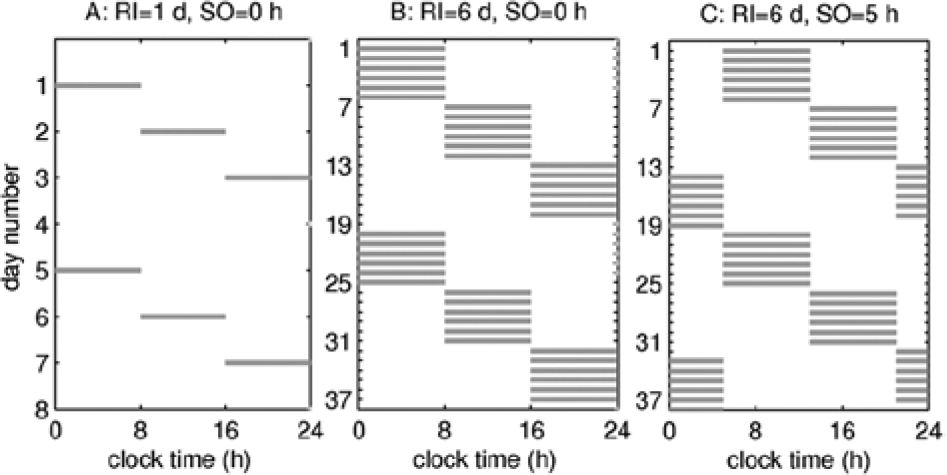
Examples of 3-shift forward rotating schedules, with shifts shown by gray stripes. Panel (A) illustrates raster for RI=1 d and SO=0 h, and thus the shifts start at 0000, 0800, and 1600. Panel (B) shows a raster for SO=0 h and RI=6 d. Panel (C) illustrates an example with RI=6 d and SO=5 h.

In order to assess the principal dynamics, we fix the direction of rotation and do not consider the effects of days off or other parameter changes. We thus aim to understand basic interdependencies that rule the dynamics to allow better shift scheduling in future.

Materials and Methods

The combined sleep-wake cycles model simulates the dynamics of the sleep-wake switch between the mutually inhibiting sleep- and wake-active neuronal populations in the brain under the effects of the homeostatic (H) and circadian (C) processes (e.g., Phillips et al., 2011; Postnova et al., 2012, 2013). It uses a simplified case of the neural field theory to model the mean electric potentials of the sleep- and wake-active neuronal populations (Phillips and Robinson, 2007). Homeostatic process H is modeled as accumulation of sleep drive during wakefulness and its dissipation during sleep. The circadian process C controls the 24-h periodicity of the sleep-wake cycles and is modeled by a Van der Pol oscillator, whose phase is adjusted by the light input according to experimentally recorded phase response curve (St. Hilaire et al., 2007). Overall, the combined model follows experimentally established connections between the light exposure, master circadian clock, and the sleep-wake switch. The model and its parts were calibrated and widely used in different conditions (Phillips and Robinson, 2007; St. Hilaire et al., 2007; Phillips et al., 2011; Postnova and Robinson, 2013; Postnova et al., 2012), including validation of the model against experimental data for circadian response to night shiftwork (Postnova et al., 2013). We provide detailed description of the model equations in the supplementary online material (SOM) and in the above studies.

Shiftwork is introduced in the model by specifying light intensity and forcing wakefulness during the shifts (see Fig. 2). Forced wakefulness is simulated by holding the mean voltages of the neuronal populations at their average waking levels (Fig. 2A), while allowing natural evolution of circadian and homeostatic processes, as shown in Figures 2B and 2C. We allow a 1-h commute time before and after the shift, during which wakefulness is enforced since most workers do not sleep while commuting.

Figure 2.

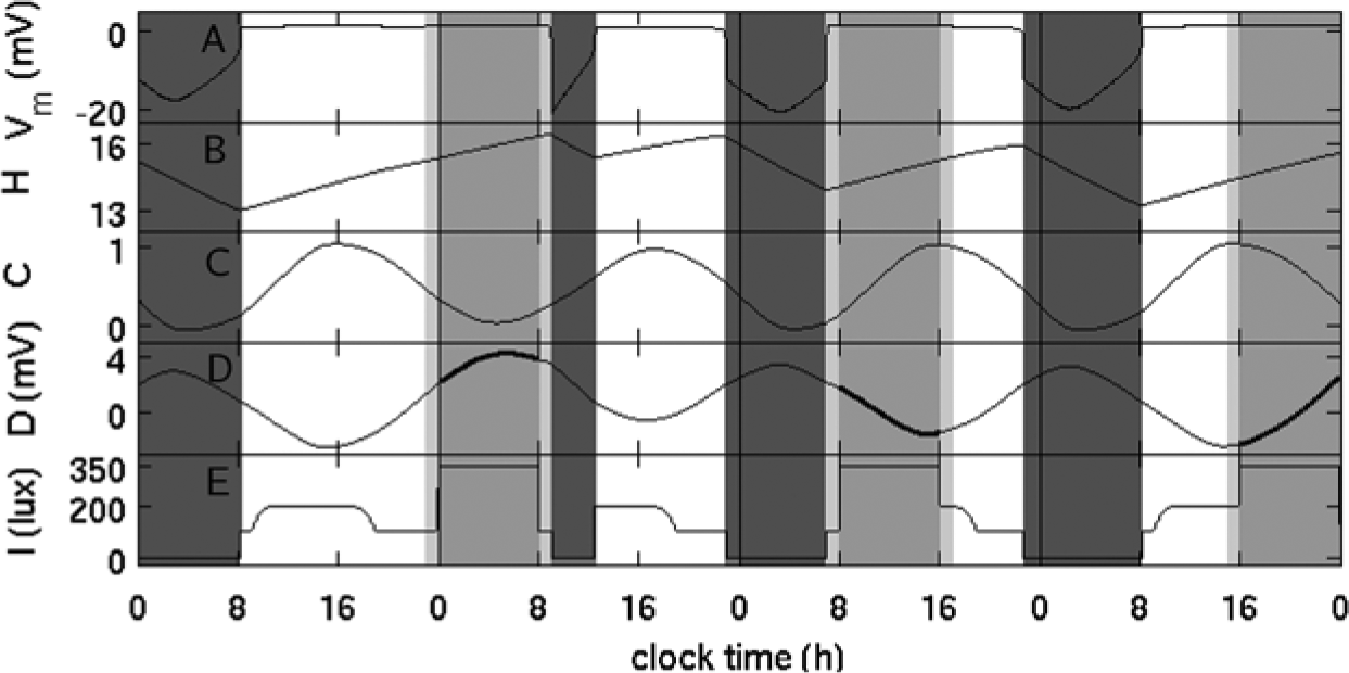
Model dynamics with shiftwork. Panel (A) shows time course of the mean voltage of the wake-active brain nuclei, (B) homeostatic process, (C) circadian drive, (D) total sleep drive, and (E) light exposure. Dark gray regions indicate sleep times, and gray regions show shifts. One-hour commute is allowed before and after the shift and shown in light gray.

The light input in the model with shiftwork is determined by environmental light, shift and commute lighting, and reduced or zero lighting during sleep, as illustrated in Figure 2E. Environmental light follows a natural light-dark cycle, which is independent of shiftwork and sleep-wake activity. The shift and sleep lighting replace environmental light during respective times, determining the actual light exposure.

In the model, we have introduced a general lighting profile with environmental light of 200 lux between 0900 and 1900 and 100 lux of artificial lighting otherwise. The transition between the two light intensities is gradual to mimic sunrise and sunset. Artificial lighting of 100 lux is chosen, since this is the common light intensity at home in the evening. The 200 lux selected during the day is much lower than natural outdoor lighting, because most people spend their days indoors. We set shift lighting to 350 lux—common for an office environment. Commute lighting is set to environmental at respective time. To mimic the reduced light level during sleep, we set it to 0 lux for simplicity, but other options could be used. Sleep times are found from the model dynamics (see SOM), so the light profile changes depending on sleep and shift times.

Mean shift sleep drive (<D_shift>) is used to compare sleepiness on different shift schedules. It is calculated by averaging the total sleep drive values (D) taken only during the shifts (bold lines in Fig. 2D) across 1 year of shiftwork. The 1-year duration of simulations is chosen to have a sufficiently high number of rotation cycles for both high and low RI to allow meaningful comparison. Before shiftwork is introduced, the model is in the state entrained to environmental lighting.

The total sleep drive reflects a physiological drive to sleep and is composed of the circadian (C) and homeostatic (H) effects on the sleep-active population in the model and is calculated as

$$D=v_{vh}H+v_{vc}C+D_0,$$

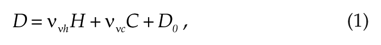
with coupling factors ν_νh>0 and ν_νc<0 reflecting sleep-promoting effects of H and wake-promoting effects of C, and D₀ is a constant reflecting base sleepiness level. Averaging the total sleep drive D across all the shifts results in one mean shift sleepiness value (<D_shift>) for each schedule, which allows easy comparison between the schedules and reflects the overall sleepiness level.

The timing of the core body temperature minimum (t_CBT) is used to mark the circadian phase for easier reference to experimental studies. According to St. Hilaire et al. (2007),

$$t_{CBT}=t_{\phi crit}+0.97,\text{with}{\text{φ}}_{crit}=-2.98=\text{arctan}\left(\frac{x}{x_C}\right),$$

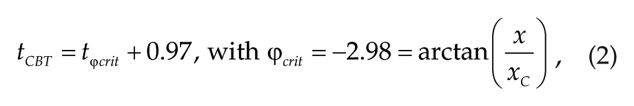
where x and x_C are the circadian variables of the model with x defining the dynamics of C. In entrained conditions, t_CBT appears 2 to 3 h before awakening and moves with the circadian drive when lighting is changed. Generally, t_CBT is close to the minimum of C but does not exactly coincide with it.

The parameters of the model are chosen to match the general case of the most common normal sleep pattern—sleep appearing between 0000 and 0800 (Rönneberg et al., 2003). The t_CBT with environmental lighting and without shiftwork appears at 0520 h. For the full list of parameters, see the SOM.

Results

In the following, we systematically study the model dynamics on shift schedules with different RI and SO. The inputs to the model are the shift schedule and the light profile, which is affected by the shift and sleep times. The outputs, based on the incorporated biological mechanisms, are the sleep-wake times, sleepiness levels (D), and circadian phase (t_CBT). In this study, we primarily use mean shift sleepiness <D_shift> to compare the overall physiological need for sleep on different schedules and t_CBT to track the changes in circadian dynamics (see Materials and Methods and SOM).

Importantly, the circadian and homeostatic processes in the model interact via modification of light input by sleep times and via circadian phase affecting sleep times. During any type of shiftwork (permanent or rotating), circadian dynamics are primarily affected by the light exposure, which changes due to the lighting introduced during the shifts as well as due to reduced or zero lighting during sleep. If entrainment to a shift is not achieved, this light profile changes every day due to changes in sleep time. This is an important feature, introducing essential and realistic dependencies that are not widely considered in other models.

Mean Shift Sleepiness

Levels of mean shift sleepiness across 1 year of shiftwork versus RI and SO are shown in Figure 3. Starting from rapid 1-day rotation (RI=1 d), mean shift sleepiness increases with RI to a peak at RI=6 d (e.g., <D_shift>=0.76 mV at RI=6 d, SO=0 h) and then decreases. At RI=9 d, <D_shift> is already lower than at RI=1 d (e.g., 0.31 vs. 0.39 mV at SO=0 h). Further increase of RI leads to gradual decrease of <D_shift>, but the rate of decrease slows down. At RI=20 d and SO=0 h, mean shift sleepiness is at −0.36 mV, which is still much higher than for daytime workers with <D_shift> = −1.76 mV (negative values refer to lower sleepiness level, as in Fig. 2). The changes of <D_shift > are qualitatively similar at different SO, as seen in Figure 3.

Figure 3.

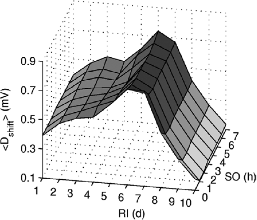
Dependence of the mean shift sleepiness across 1 year of shiftwork (<D_shift>) on SO and RI. Shading of the surface additionally indicates levels of <D_shift>, with higher values in darker color.

In the following sections, we explore the mechanisms underlying the changes of sleepiness in Figure 3 with a primary focus on the circadian dynamics.

Effects of Rotation Interval on Circadian Dynamics

Rotating schedules introduce 2 periodic inputs acting on the circadian system. The first one is the individual shifts, with each shift appearing with a 1-day period for RI days. Entrainment to a shift is achieved when RI is sufficient to bring the circadian oscillator to its stable state. Second is the rotation schedule, which has all 3 shift types with the total period equal to the RC. Entrainment to a schedule is observed when the circadian dynamics repeats with RC. Note that the system can be entrained to the schedule without entraining to each shift type separately. However, entrainment to each shift type means that the dynamics also repeat with RC.

Figure 4 demonstrates an example of the effects of RI on timing of the core body temperature minimum (t_CBT), which is used as a marker of circadian phase and is generally positioned close to the maximum sleep drive (D). The illustrated example is for SO=0 h, but the dynamics are qualitatively similar at other SO (e.g., see SOM for SO=5 h). In conditions entrained to environmental light and without shiftwork, t_CBT is stable at 0520 h (i.e., about 2.6 h before awakening).

Figure 4.

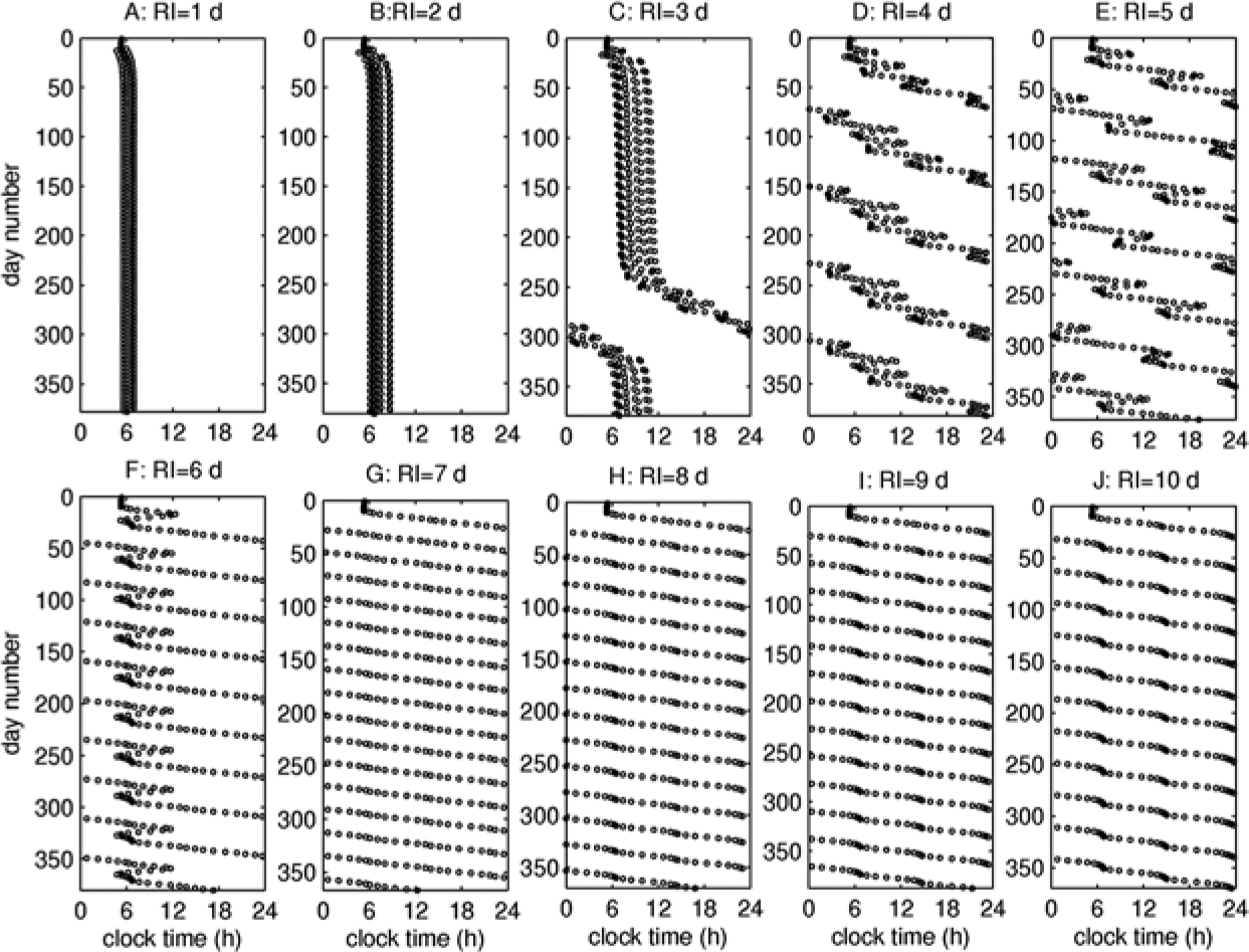
Timing of the core body temperature minimum (t_CBT) on schedules with different RI. Panels A to K correspond to RI=1-10 d at SO=0 h. Duration of simulations is close to 1 year but differs slightly for different RI in order to contain an integer number of RCs.

For rapid shift rotation at RI=1,2 d, shown in Figures 4A and 4B, t_CBT changes only slightly, fluctuating within a narrow interval with a period of RC after the initial convergence is achieved. The distribution in Figure 4B is broader than in Figure 4A, because more days spent on each shift allow larger changes of t_CBT. Increase of RI to 3 days distorts these dynamics and leads to gradual delay of t_CBT with each RC, resulting in an around-the-clock transition at the end of the year. The rate of such transitions increases with RI. An important feature is that for RI≥7 d, t_CBT starts to delay on every shift, whereas it demonstrates both advance and delay at lower RI. This transition is associated with the highest sleepiness in Figure 3.

The periodicity of t_CBT dynamics at RI=1,2 d and RI≥6 d in Figures 4A, 4B, and 4F-4J indicates that the system entrains to the shift schedule. This is particularly clear in Figure 5, which shows t_CBT after each RC for 6 years of shiftwork. When entrainment to one or more RC is achieved, multiple t_CBT values overlap. For the system entrained to one RC, the result is a single point for the respective RI in Figure 5. This is observed for the RI=1,2 d and RI≥7 d. At RI=6 d, Figure 5 shows two points, instead of one, indicating that the system is entrained to 2 RC, repeating dynamics every 38 days. At intermediate RI=3-5 d, the t_CBT values are distributed across the entire 24-h interval, indicating that no entrainment to the schedule is achieved or the period of entrainment is very long.

Figure 5.

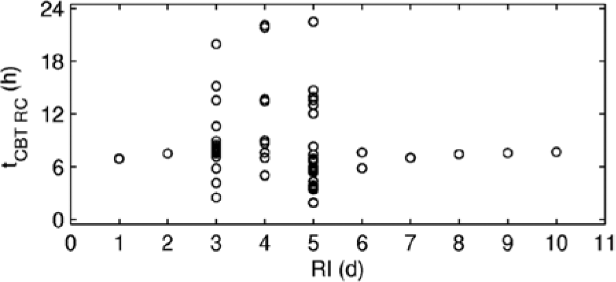
Position of t_CBT after each RC (1 point per RC) for 6 years of shiftwork at different RI at SO=0 h. The first month of transient dynamics is removed for all rotation intervals to show stable dynamics where it exists.

The results in Figures 3 to 5 confirm experimental studies showing that low RI result in only minor changes of the circadian phase, while high RI are close to reentraining the circadian oscillator to the shift schedule; both are associated with reduced sleepiness compared to intermediate RI (e.g., Viitasalo et al., 2008; Härmä et al., 2006; De Valck et al., 2007; Knauth, 1993, 1995; Bambra et al., 2008). However, for the first time, here we systematically show the effects of RI and demonstrate that the inability to entrain on the shift schedules with intermediate RI=3-5 d is intrinsic to the system and is not related to such external disturbances as social commitments, days off, and other activities that are often blamed for workers’ inability to adapt.

Noteworthy, these un-entrained dynamics at intermediate RI are not observed when the circadian and sleep systems are uncoupled, that is, when lighting during sleep is equal to environmental light (unpublished simulations). This confirms the importance of using the combined model to study shiftwork.

Mechanisms: The Shift Response Map

The key question is the following: what are the mechanisms behind the dynamics in Figures 3 to 5? Depending on the shift start time relative to the circadian phase, the circadian oscillator either advances or delays to achieve reentrainment (e.g., Golombek and Rosenstein, 2010). However, for the rotating shifts, the initial circadian phase on each new shift after changeover is different, depending on the dynamics on prior shifts, and can be anywhere between 0 and 24 h. Thus, to fully describe the circadian response to shifts in the system, we need to know the direction of t_CBT change on a shift starting anywhere between 0 and 24 h with initial t_CBT between 0 and 24 h. The map illustrating this is shown in Figure 6, and a full description of its calculation is in the SOM.

Figure 6.

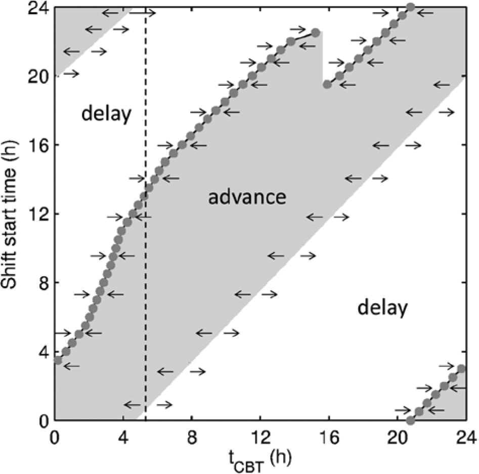
Shift response map for t_CBT depending on initial t_CBT and shift start time. Gray area corresponds to advance region and white to delay, with arrows demonstrating the direction of t_CBT change. Circles show stable $t_{CBT}^{*}$ achieved when the system is entrained to the corresponding shift. Dashed line shows $t_{CBT}^{*}$ when the system is entrained to environmental light without shiftwork (i.e., $t_{CBT}^{*}$ =05:20 h).

The map shows the shift start times leading to advance and delay of t_CBT when starting from any initial t_CBT. The gray circles demonstrate the timing of entrained t_CBT ( $t_{CBT}^{*}$ ), for each of the shift start times; that is, when shift with the respective start time is introduced in the system with the initial t_CBT = $t_{CBT}^{*}$ , no change of t_CBT is observed. In this case, if a permanent shift schedule with this shift start time is introduced, the system will remain in this entrained state. If for a given shift start time, the initial t_CBT is on the right of its $t_{CBT}^{*}$ (gray area), the t_CBT advances to reach $t_{CBT}^{*}$ ; it delays if the initial t_CBT is on the left of $t_{CBT}^{*}$ (white area). The map does not provide the information on the magnitude of t_CBT change introduced by one shift, but according to the circadian phase response to light (e.g., Golombek and Rosenstein, 2010), it can be expected that the rate of change is larger when the t_CBT is further away from its $t_{CBT}^{*}$ and reduces when the stable state is near. The right border of the advance region represents unstable states for t_CBT from which the system repels toward its stable position on the left border.

Remarkably, the shifts starting between 1930 and 2230 h have two stable $t_{CBT}^{*}$ values. The earlier one is associated with sleep stabilizing directly after commute from a shift and the later one with sleep stabilizing directly before commute to a shift. Only one bunch of stable states was observed for permanent shifts (Postnova et al., 2012), because only the earlier $t_{CBT}^{*}$ is achieved when the system starts from the circadian position entrained to the environmental light (i.e., from $t_{CBT}^{*}$ = 0520 h).

In the case of forward rotating shifts, it can be expected that for the schedules with SO=3.5-6.5 h, the t_CBT on the shifts starting between 1930 and 2230 h can fall into the basin of attraction of any of the two $t_{CBT}^{*}$ . However, we find only minor differences in dynamics on these schedules compared to those that do not include the bistability region (see SOM Fig. S1); for example, the number of around-the-clock transitions per year at RI=3 d is increased from 1 at SO=0 h to 3 at SO=5 h. However, the qualitative dynamics (i.e., the periodic circadian regimes at low and high RI, as well as the un-entrained circadian rhythms at intermediate) are preserved.

Key Dynamics on 3-Shift Forward Rotating Schedules

The shift response map in Figure 6 can now be used to understand the circadian dynamics in Figure 4. The schedule in Figure 4 has SO=0 h and thus the shift start times of 0000, 0800, and 1600. Accordingly, the initial t_CBT values and dynamics on each new shift depend on the t_CBT value achieved on the last day of the prior shift. For example, from the map, it is seen that t_CBT advances on the 0800 shift if the initial t_CBT is in the 0255- to 1250-h interval and delays otherwise. Thus, the t_CBT value on the last 0000 shift, before the changeover to 0800, in the 0255- to 1250-h interval leads to advance on the 0800 shift and to delay if it is outside this interval.

On each shift, t_CBT moves toward its stable value, but the overall dynamics depend on RI. Significant changes in dynamics happen when RI is such that t_CBT change on a given shift is sufficient to induce a transition between advance and delay on the next shifts, which ultimately leads to the complex dynamics in Figure 4.

Rapid rotation at RI=1,2 d introduces only minor changes in t_CBT, which is initially entrained to the environmental light. An example of such dynamics is shown in Figures 7A and A′ for RI=2 d. The initial state of t_CBT = 0520 h falls into the delay region for the 0000 and 1600 shifts, but in the advance region for the 0800 shift. Thus, the map in Figure 7A predicts that t_CBT advances on the 0800 shift (arrow 2) and delays on the 0000 and 1600 shifts only (arrows 1 and 3). This is confirmed by the t_CBT time series in Figure 7A′, which shows 3 RC taken at the end of the year in Figure 4A. In this case, the delay is balanced by advance during 1 RC and t_CBT changes following a closed trajectory in the map with a period of 1 RC.

Figure 7.

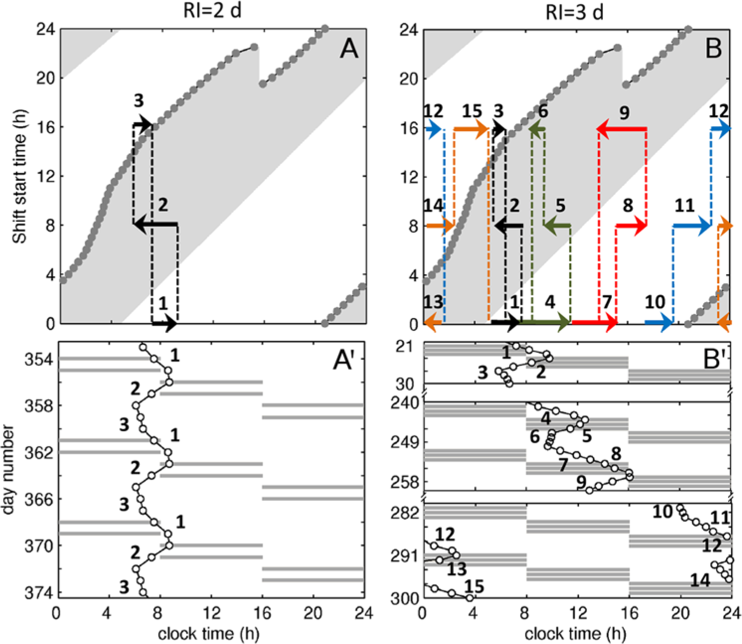
Key dynamics at low and intermediate RI. Panel (A) shows predicted t_CBT trajectories on the shift response map and (A′) t_CBT time series observed at RI=2 d, SO=0 h. Similarly, panels (B) and (B′) show the t_CBT trajectories and selected time series for RI=3 d, SO=0 h. In (A) and (B), arrows show the predicted direction of t_CBT change on 0000, 0800, and 1600 shifts. Dashed lines indicate changeover from one shift to the next. Dark gray lines in (A′) and (B′) indicate shifts, and empty circles show the position of t_CBT on a given day, which are taken from Figures 4B and 4C. Numbers show the order of events in all panels. In (B), the trajectories are additionally emphasized with different shades of gray (colors online). In order to avoid arrow overlap and reduction of trajectories’ readability in (B), the arrows show the qualitative dynamics but not the exact quantitative change of t_CBT with respect to (B′).

RI=3 d is long enough for t_CBT to start crossing the borders of the advance and delay regions and, thus, introduce changes in the dynamics, as shown in Figures 7B and 7B′. The key features in the order of their appearance are as follows:

Gradual delay of t_CBT with each RC

Longer RI leads to stronger delay of t_CBT on the 0000 shift compared to the RI=2 d case. This results in delaying the initial t_CBT for the 0800 shift, which leads to a likewise delayed start on the 1600 shift, bringing it closer to its entrained position $t_{CBT}^{*}$ . This further delays t_CBT on the 0000 shift of the next RC, resulting in an even later starting time on the 0800 shift. Altogether, this moves the 1-3 t_CBT trajectory in Figure 7B to a later time with each RC, resulting in its slow drift, as also seen in Figure 7B′.

Delay→advance transition on the 1600 shift

At some point, the above changes become sufficient to delay the t_CBT on the 0000 (arrow 4) and 0800 (arrow 5) shifts so much that they bring initial t_CBT on the 1600 shift to the right of its $t_{CBT}^{*}$ (arrow 6), thus changing the dynamics from delay to advance; compare the time series 1-3 and 4-6 in Figure 7B′.

Advance→delay transition on the 0800 shift

The above transition of t_CBT on the 1600 shift to the advance area (arrow 6) moves the starting t_CBT for the 0000 shifts even later. This later t_CBT on the 0000 shift brings the final t_CBT on the 0800 and 1600 shifts to later times with every RC, dragging them further from $t_{CBT}^{*}$ . Ultimately, the delay on the 0000 shift is so large (arrow 7) that it leads to a change from advance to delay on the 0800 shift (arrow 8), with t_CBT still advancing on the 1600 shift (arrow 9). This corresponds to the change of the t_CBT time series in Figure 7B′ from the interval indicated with 4-6 to 7-9.

Advance→delay transition on the 1600 shift

The combined delay on the 0000 and 0800 shifts as in trajectory 7-9 is significantly greater than the advance on the 1600 shift, leading to even faster delay of the overall trajectory. This ultimately leads to initial t_CBT on the 1600 shift crossing the right border of the advance region, changing the dynamics on this shift to delay (trajectory 10-12 in Fig. 7B). This results in t_CBT moving into the next day on the 1600 shift and corresponds to the around-the-clock transition in Figure 4C, which is enlarged in Figure 7B′.

Delay→advance and advance→delay transitions on the 0000 shift

The delay of t_CBT on the 1600 shift brings initial t_CBT for the 0000 shifts inside its advance region (arrow 13), leading to change in dynamics from delay to advance. This induces an additional around-the-clock transition but opposite in direction. The t_CBT continues to delay on both the 1600 and 0800 shifts (arrows 14 and 15), and thus after a number of RC, it is sufficient to return the dynamics on the 0000 shift to delay, as shown by the arrow 1 in Figure 7B. After that, the dynamics return to a zone with slow drift of t_CBT, and the above steps repeat.

The above dynamics are also observed for RI=4,5 d, with larger RI leading to more frequent around-the-clock transitions and shorter drift time, as seen in Figures 4D and 4E. For the SO, including the bistable region, there will be additional dynamics when t_CBT falls inside the basin of attraction for the second stable state, which will initiate more advance/delay transitions due to a larger number of transition borders (see SOM Fig. S1).

RI=6 d is sufficiently large to avoid most of the transitions observed at RI=3-5 d by bringing the initial t_CBT on the 0000 and 1600 shifts fully into delay regions, as shown in Figure 8A (arrows 1,3 and 4,6). However, on the 0000 shift, the RI=6 d brings t_CBT very close to the transition border for the 0800 shift. Crossing the right border of the advance region on the 0800 shift with every RC leads to delay of t_CBT in 1 RC (arrow 2) and its advance in the next (arrow 5), thus producing the period-2 behavior seen in Figures 8A′, 4F, and 5.

Figure 8.

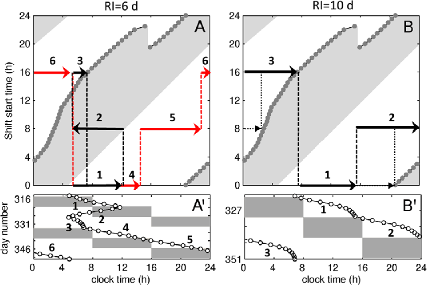
Key dynamics at intermediate and high RI. Panel (A) shows predicted t_CBT trajectories on the shift response map and (A′) t_CBT time series observed at RI=6 d, SO=0 h. Similarly, panels (B) and (B′) show the t_CBT trajectories and time series for RI=10 d, SO=0 h. The time series in (A′) and (B′) are taken from Figures 4F and 4J, respectively. The black and gray arrows in (A) (black and red online) emphasize the two different trajectories. The dotted lines in (B) show the predicted dynamics when entrainment to every shift in the schedule is achieved. All other notations are the same as in Figure 7.

Slow rotation at RI≥7 d is sufficient to bring initial t_CBT for each shift type fully inside the delay region, as seen in Figure 8B, resulting in stable delay-only dynamics shown in Figure 8B′. Noteworthy, entrainment to each shift type is not achieved even for RI=10 d. For example, for the 0000 shift, $t_{CBT}^{*}$ = 2044, but the t_CBT value achieved on the latest 0000 shift at RI=10 d is at 1502 h (Fig. 8B′). The predicted entrained trajectory, which can be achieved at sufficiently high RI, is shown with dotted lines in Figure 8B.

Overall, here we use the shift response map to explain the qualitative dynamics on different schedules. In theory, it can also be used to predict dynamics without the need for simulations, but to do so, it has to account for the rate of t_CBT change per shift-day and for the circadian dynamics during changeovers. These features may be incorporated in the future.

Contribution of the Circadian Activity and Sleep Time to Mean Shift Sleepiness

The profile of mean shift sleepiness in Figure 3 is determined by the relation between shift times, circadian phase, and sleep duration. When t_CBT appears during the shift, it means that sleepiness is high during this shift because it is scheduled during low circadian activity. The worst circadian timing of an individual shift is when it is fully positioned at the time of physiologically expected sleep time (i.e., in the model, this is observed when t_CBT appears 2.6 h before the end of the shift). Thus, the schedules having t_CBT during the shifts (e.g., those in Figs. 7B′ and 8A′) have higher sleepiness than those with t_CBT mostly outside shifts.

The duration of sleep on the schedules is also determined by the relation between t_CBT and shift time. If the shift appears during low circadian activity, then sleep is allowed only during high circadian activity, and thus sleep duration is reduced, further contributing to the increased sleepiness. When such a situation is repeated for a number of days, sleep debt accumulates, increasing sleepiness with each additional shift-day. As can be expected, the profile of mean sleep duration across shift schedules is negatively correlated with the mean shift sleepiness (more details are in the SOM).

Discussion

We have systematically examined the effects of RI and SO on sleepiness and circadian dynamics on forward rotating 3-shift systems using a mathematical model. Most important, we have explained the mechanisms behind the observed dynamics through developing a shift response map that allows tracking circadian response to a shift depending on shift start time and circadian phase. Below we discuss specific results, applications, and limitations.

Mean shift sleepiness is highest for RI=3-7 d with a peak at RI=6 d, and thus these rotation intervals are not advisable. Mean shift sleepiness on the slow rotating schedules with RI≥9 d is lower than on rapid ones with RI=1 d. However, slow rotation leads to continuous delay of the circadian oscillator, and frequent circadian changes were demonstrated to reduce longevity in animal experiments (Saint Paul and Aschoff, 1978; Davidson et al., 2006). Thus, even though sleepiness at slow rotation is shown to be lower, further understanding of the effects of frequent circadian reentrainment on human health is needed to decide whether rapid or slow rotation is better.

Circadian rhythms are found to entrain to shift schedules at low (1,2 d) and high RI (≥7 d), demonstrating periodic changes with each RC. However, at RI=3-5 d, the system is unable to entrain even in the absence of any external factors, such as social commitments or days off, which are often blamed for workers’ inability to adapt to a schedule. Furthermore, even at RI=10 d, entrainment to each shift in the schedule is not achieved, indicating that in a realistic situation with multiple disturbances, entrainment on rotating schedules is even harder to achieve without specifically developed treatments (e.g., bright light therapy).

Shift offset was found to have a weak effect on the mean shift sleepiness, which is surprising given the bistability region for SO=3.5-6.5 h in the shift response map. This is likely to be explained by two factors: (1) the used sleepiness measure and (2) lack of entrainment to the shifts. The mean shift sleepiness is averaged across all 3 shift types in the schedule, thus including night, day, and morning shifts and smoothing out the differences introduced by the shift start times. Furthermore, the lack of entrainment is the main contribution to <D_shift>, so it is expected that at higher RI, effects of SO are more prominent (see confirmation in SOM). These variable effects of SO on sleepiness may explain the inconsistency of experimental observations, with some data showing no effects of SO on sleepiness and others indicating significant effects (e.g., Knauth, 1993; Rosa et al., 1996).

Most important, we were able to explain the mechanisms behind the circadian dynamics observed on the schedules. We have developed a shift response map illustrating the circadian response depending on the relation between the circadian phase and the shift start time. This relation and the amount of circadian change achieved per shift-day define the dynamics on each shift. Note that this map reflects the basic properties of the system in the specified light conditions and is not limited to the shift schedules considered here. Thus, it can potentially aid in the development of shift schedules with desired circadian dynamics. For example, consider the case of RI=3 d at SO=0 h, where the dynamics are not entrained. From the map, it can be predicted that stronger advance on the 0800 shift can be sufficient to balance the delay on the 0000 and 1600 shifts, thereby reaching periodic dynamics and avoiding around-the-clock transitions. This stronger advance can be reached either by adding more days on the 0800 shift, while leaving the number of 0000 and 1600 shifts the same, or increasing light intensity on the 0800 shift, thereby increasing the entrainment rate.

Different shift light intensities are expected to not change the map significantly, as long as they are above the daylight levels. However, shift lighting affects the rate of circadian change per shift-day and can thus move the sleepiness surface in Figure 3 to the right for lower shift lighting or to the left for higher. For example, shift light intensity of 10,000 lux is sufficient to induce un-entrained circadian dynamics already at RI=2 d, instead of RI=3 d (unpublished simulations). Thus, even though bright light was shown to improve adaptation to permanent night shifts (e.g., Czeisler et al., 1990; Postnova et al., 2013), this improved reentrainment to each shift may be a disadvantage in the rotating schedule. Conversely, at intermediate RI, increased lighting may be sufficient to entrain to the shift schedule and thereby reduce sleepiness, but this needs to be studied in more detail. Note that shift lighting below environmental light qualitatively changes the principal shape of the light profile and may significantly change $t_{CBT}^{*}$ and the map.

Overall, in this study, we have uncovered some of the general mechanisms involved in response to rotating shiftwork, which may allow for better shift scheduling in the future. However, it should be applied keeping in mind its limitations. Quantitative response to the forward rotating schedules depends on the model parameter set and light profile. The study was done for a parameter set chosen to fit a most common sleep pattern, a specific shift duration of 8 h, and an exemplar lighting profile; we also did not consider the effects of noise or days off. More research is needed to understand how these parameters affect the shift response map and the dynamics on rotating schedules.

Different parameters are of interest in different situations and experimental protocols. The advantage of the modeling approach is that the system can be easily calculated for conditions of interest. To allow such case-specific application of the model, we have developed software where custom protocols can be incorporated and examined directly by users (www.sleepsim.com).