Exploring Sleepiness and Entrainment on Permanent Shift Schedules in a Physiologically Based Model

Abstract

The effects of permanent shift work on entrainment and sleepiness are examined using a mathematical model that combines a model of sleep-wake switch in the brain with a model of the human circadian pacemaker entrained by light and nonphotic inputs. The model is applied to 8-hour permanent shift schedules to understand the basic mechanisms underlying changes of entrainment and sleepiness. Average sleepiness is shown to increase during the first days on the night and evening schedules, that is, shift start times between 0000 to 0700 h and 1500 to 2200 h, respectively. After the initial increase, sleepiness decreases and stabilizes via circadian re-entrainment to the cues provided by the shifts. The increase in sleepiness until entrainment is achieved is strongly correlated with the phase difference between a circadian oscillator entrained to the ambient light and one entrained to the shift schedule. The higher this phase difference, the larger the initial increase in sleepiness. When entrainment is achieved, sleepiness stabilizes and is the same for different shift onsets within the night or evening schedules. The simulations reveal the presence of a critical shift onset around 2300 h that separates schedules, leading to phase advance (night shifts) and phase delay (evening shifts) of the circadian pacemaker. Shifts starting around this time take longest to entrain and are expected to be the worst for long-term sleepiness and well-being of the workers. Surprisingly, we have found that the circadian pacemaker entrains faster to night schedules than to evening ones. This is explained by the longer photoperiod on night schedules compared to evening. In practice, this phenomenon is difficult to see due to days off on which workers switch to free sleep-wake activity. With weekends, the model predicts that entrainment is never achieved on evening and night schedules unless the workers follow the same sleep routine during weekends as during work days. Overall, the model supports experimental observations, providing new insights into the mechanisms and allowing the examination of conditions that are not accessible experimentally.

Shift work has become an integral part of modern life. An estimated 20% of the US workforce engages in permanent evening/night or rotating shift systems (McMenamin, 2007), and the situation is similar in other industrialized countries. Such shift schedules necessarily involve wakefulness outside normal daylight hours and are inherently opposed to natural biological rhythms. One dangerous complication of shift work is excessive sleepiness during work hours that frequently culminates in accidents (Åkerstedt, 1995; Dinges, 1995). Furthermore, due to diverse disturbances of sleep-wake cycles, workers can stay unentrained to their work schedule for many years, which affects their health and leads to chronically high levels of sleepiness (Folkard et al., 2005; Boivin et al., 2007). Better understanding of the mechanisms underlying shift workers’ sleepiness and prediction of ease of adaptation to particular schedules would prove highly valuable for the development of measures decreasing sleepiness and improving the well-being of shift workers. Such predictions and studies of the mechanisms can be made using mathematical models of sleepiness and performance (Achermann and Borbély, 1992; Jewett and Kronauer, 1999; Mallis et al., 2004; Hursh et al., 2004; Olofsen et al., 2010; Ishiura et al., 2007; and references therein), most of which were fitted to experimental data and successfully predicted some aspects of sleepiness and performance during shift work.

All sleep models embody the 2-process concept in which sleep-wake cycles are controlled by the interaction between circadian and homeostatic processes in the brain (Borbély, 1982). The circadian component provides a 24-hour periodicity of bodily processes and helps to promote wakefulness (Moore, 2007; Rosenwasser, 2009). The homeostatic component depends on the time spent awake and is responsible for the accumulation of sleep pressure during wakefulness and its recovery during sleep (Borbély, 1982). Interaction between these processes is thought to determine sleepiness and thereby influence performance and fatigue (Van Dongen and Dinges, 2000).

The homeostatic and circadian processes, and thus the sleepiness during shift work schedules, are mutually coupled with a large number of interacting processes, creating a multitude of positive and negative feedback loops. In the simplest case, those include light on the shifts and on the breaks and nonphotic inputs during wakefulness such as food and locomotion. These re-entrain the circadian process, thereby changing total sleep drive and sleepiness. In turn, sleep drive affects sleep times, thus closing the loop by modifying homeostatic pressure, light, and nonphotic inputs. Most of the existing models, although making good quantitative predictions, do not account for such nonlinear interactions or are not directly based on physiology, which makes it difficult to examine the mechanisms behind adaptation to particular shift schedules or increase of sleepiness.

In the present study, we aim to understand the mechanisms behind sleepiness and entrainment on different shift schedules, accounting for dynamic changes in zeitgebers (time givers) as well as homeostatic and circadian processes. For this purpose, we use the physiologically based mathematical model of sleep-wake cycles that combines the model of sleep-wake switch of Phillips and Robinson (2007) with the human circadian pacemaker model of St. Hilaire et al. (2007). This combined model and its modifications had already been used to study other phenomena, such as forced desynchrony (Phillips et al., 2011) or mechanisms of different chronotypes (Phillips et al., 2010), and showed a good agreement with experimental data. In the study of chronotypes, a simpler version of the human circadian pacemaker model by Forger et al. (1999) was used instead of the St. Hilaire et al. (2007) model. These circadian models are similar, with the major difference being the addition of a nonphotic component in the St. Hilaire et al. (2007) model, which gives a better fit to experimental data. Thus, we have chosen this most recent version for our study. The Phillips and Robinson (2007) model accounts for the physiological mechanisms of the sleep-wake switch as described in Saper et al. (2010) and was also extensively studied and fitted to experimental data (Phillips and Robinson, 2007, 2008; Fulcher et al., 2010). Thus, in this study, we do not develop a new model but apply an established, validated one that is known to work properly in different conditions.

There are numerous different shift schedules and conditions: workers can be on rotating or permanent schedules, they can be exposed to bright or dim light, or lighting may change depending on weather or season. Many such conditions can be implemented in the model. However, in order to be able to understand the model’s dynamics, it is first necessary to study simple schedules that allow easy access to the underlying mechanisms. Therefore, in the present study, we apply the model to the simplest case of permanent shift schedules with a duration of 8 hours placed at different times of the day. We examine entrainment and sleepiness on such schedules, along with the effects of noise and days off. Understanding the model’s dynamics in this simple case will allow us to make predictions about more complicated and realistic schedules and develop measures to reduce sleepiness.

Materials and Methods

Both the Phillips and Robinson (2007) model of the sleep-wake switch and St. Hilaire et al. (2007) model of the human circadian pacemaker are described in detail in the original works. The combined version of the model in different modifications is also given (Phillips et al., 2010, 2011). For completeness, we present all equations and parameter values for the combined model in the supplementary online material (SOM). Therefore, here, we give only a brief description of its structure.

A schematic of the combined model is shown in Figure 1. The sleep-wake switch part of the model (Fig. 1, upper) simulates reciprocal inhibition between the monoaminergic nuclei of the brainstem (MA) and the ventrolateral preoptic nucleus of the hypothalamus (VLPO), which results in the flip-flop transition between sleep and wakefulness (Saper et al., 2010). The effects of orexinergic, cholinergic, and other neuronal populations are all combined in a simplified constant input A to the MA. The dynamics of the monoaminergic and hypothalamic neurons are modeled using a neural field approach, which simulates the activity of the entire population based on the average firing rates and membrane potentials. Timing of the switch between the activity of the MA and VLPO is controlled by the homeostatic (H) and circadian (C) drives, whose influence is introduced as inputs to the VLPO with H promoting and C inhibiting its firing activity. This results in an abrupt flip-flop–like switch between the high VLPO/low MA firing during sleep and low VLPO/high MA activity during wakefulness.

Figure 1.

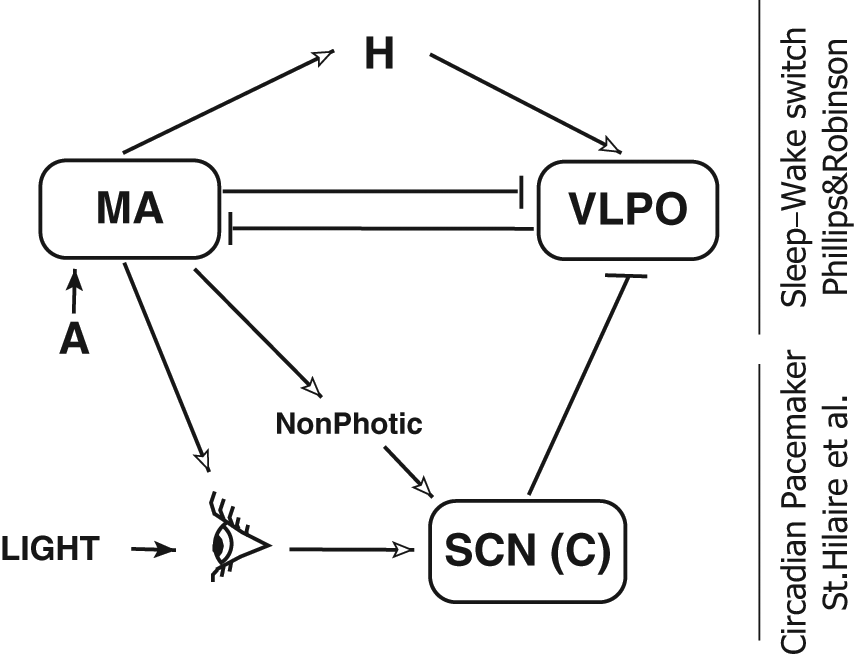
Schematic of the model, combining the sleep-wake switch model of Phillips and Robinson (2007) and the human circadian pacemaker model of St. Hilaire et al. (2007). MA = wake-active monoaminergic nuclei of the brain stem and hypothalamus; VLPO = sleep-active ventrolateral preoptic nucleus of the hypothalamus; SCN = suprachiasmatic nucleus of the hypothalamus, providing circadian drive C; H = homeostatic drive; A = external stimuli from other neuronal populations. Bar-headed lines correspond to inhibitory connections, while arrows correspond to excitatory connections.

In the model, dynamics of H depend on the firing rate of the MA population. When MA is active and mean firing rate is high (wake state), H is increasing, while it is decreasing when activity of MA is low (sleep). This behavior is similar to that of the 2-process model (Daan et al., 1984); however, here, exponential saturation and relaxation of the homeostatic drive emerge from the modeled brain activity and are not inserted as an exponential function (see SOM for equations). The circadian drive (C) is simulated by the St. Hilaire et al. (2007) model, which is the most recent modification of the circadian pacemaker models developed in Kronauer’s group (Kronauer et al., 1999; Jewett et al., 1999).

The St. Hilaire et al. (2007) model simulates activity of the circadian pacemaker in the form of a Van der Pol oscillator that has an endogenous period of approximately 24 hours and can be adjusted to different values if required for other applications. The endogenous oscillations of this pacemaker are entrained by photic and nonphotic zeitgebers (see inputs to the SCN in Fig. 1). The nonphotic stimuli are modeled in a simple way by introducing a stronger stimulation of the SCN during wakefulness than during sleep. Photic input has a more complicated form that accounts for the experimentally demonstrated physiological pathways (reviewed in Golombek and Rosenstein, 2010). Light intensity to which a subject is exposed is introduced as an input to the model, which leads to activation of photoreceptors in the retina. The number of activated receptors depends on the light intensity and availability of photoreceptors that are ready to be activated, where the latter is determined by the previous light input. After the receptors have been activated, they send a signal to the circadian oscillator. This affects the amplitude of the pacemaker and modifies its phase. Finally, the effect of light on the phase also depends on the actual state of the circadian oscillator, that is, on the phase itself.

Together, the homeostatic (H) and circadian (C) drives determine a total sleep drive D acting on the VLPO and controlling the sleep-wake transitions. This sleep drive is calculated by the formula

$$D=v_{vh}H+v_{vc}C+D_0,$$

(1)

where ν _vh and ν _vc are the strengths with which H promotes (ν _vh > 0) and C inhibits (ν _vc < 0) firing activity of the VLPO, and D₀ is a background level of sleep propensity (see SOM for details). Accordingly, D can be either positive or negative depending on whether H or C prevails. We assume here that sleepiness is determined by the total sleep drive D.

The influence of C on the VLPO is not the only connection between the 2 parts of the model (Fig. 1). The light falling on the retina, and hence affecting circadian phase, depends on the activity state of the MA, that is, whether the system is in wake or sleep state. If activity of the MA is low, meaning a sleep state, the eyelids are closed, and light input is assumed to be zero because people tend to close curtains and reduce light by other means when going to sleep. Also, the nonphotic input depends on the activity level of the MA, introducing higher input during wakefulness and lower during sleep. Such connections provide realistic nonlinear interactions between sleep-wake cycles and external cues.

In order to implement shift work, we artificially keep activity of the MA and VLPO at their wake levels during the work time, assuming that sleep is not allowed during the shifts. Additionally, we introduce lighting during the shifts, irrespective of their timing. For estimation of entrainment, we calculate the difference between the phase of the circadian oscillator on the shift schedule and the one entrained to the ambient light without shifts:

$$\Delta {\phi }_C={\phi }_{Cshift}-{\phi }_{C0}.$$

(2)

We consider entrainment to be achieved on the day_e since the start of the shift schedule when

$$|\Delta {\phi }_C(da{y}_e)-\Delta {\phi }_C(\infty )|<{\phi }_{e^{\prime }}$$

(3)

for all days > day_e, where Δϕ _C (∞) is the value of Δϕ _C to which the system settles, and ϕ _e = 10 minutes is threshold used.

Results

Understanding the effects of permanent shifts in schedules on sleepiness and re-entrainment requires an understanding of normal model dynamics. Therefore, we first demonstrate how sleep-wake cycles are generated by the combined model in the absence of shift work.

For simplicity, we set ambient light intensity to an average indoor lighting level of 200 lux between 0800 and 2200 h. Outside this time, the light input is zero, indicating night time, which can be seen in the first 2 days of the light intensity plot in Figure 2F. Such ambient light results in stable sleep-wake cycles with sleep between 2330 and 0730 h. This is demonstrated by the black lines in the activity plot of the first 2 days in Figure 2G and indicated by the periods of low firing activity of the MA and high firing activity of the VLPO in Figure 2A and 2B. The circadian variable C in Figure 2D is entrained to this light input, and maximum circadian input appears around 1500 h, which is the middle of the light interval.

Figure 2.

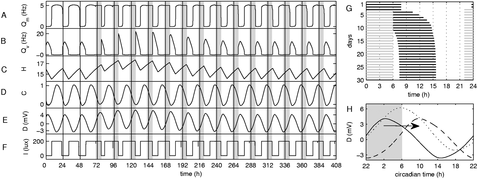
Dynamics of the model with and without shift work. Permanent shifts are introduced on the third day of the simulation between 2200 and 0600 h (indicated by shaded areas). Variables shown are mean firing rates across the neurons in (A) monoaminergic and (B) ventrolateral preoptic nuclei, (C) homeostatic sleep drive, (D) circadian process, (E) total sleep drive, and (F) light intensity. The activity diagram (G) demonstrates how sleep-wake timing is affected by shifts. Black lines correspond to sleep intervals, and gray lines correspond to shift work. (H) The effects of shift work by comparing the sleep drives on different days: solid line corresponds to the sleep drive that starts at 2200 h on day 2 and ends at 2200 h on day 3, dotted line corresponds to days 5 to 6, and dashed line corresponds to days 15 to 16 of the simulation. Arrow shows the direction of re-entrainment.

The homeostatic pressure H increases during wakefulness (see wake intervals in Fig. 2C) until, in combination with the circadian variation of C (Fig. 2D), as per equation 1, it gives such a strong total sleep drive D that sleep is initiated, as demonstrated in Figure 2E. This is seen in high firing activity of the VLPO and silence of the MA. During sleep, H decreases, while C first decreases and then increases, having its minimum in the night. This leads to increase of the total sleep drive in the first hours of sleep and then to its gradual decrease. Finally, when D is low, input to the VLPO becomes insufficient to sustain sleep, and wakefulness is initiated; that is, the VLPO is silenced, and the MA is activated.

Nonlinear Interactions on Permanent Shift Schedules

In order to demonstrate the changes that shift work introduces in the homeostatic and circadian drives, we consider an example of an evening shift starting at 2200 h on the third day of the simulation (Fig. 2). For simplicity, lighting during the work hours is set to the same 200-lux intensity as the ambient lighting. To avoid confusion here and further in the text, we use the term “ambient light” for the background 200-lux lighting from 0800 until 2200 h, which is present irrespective of work schedule. The light introduced during shift work we call “shift light”. Throughout all simulations, light is assumed to be 0 lux during sleep, irrespective of the time of the day when sleep occurs.

Shift work starting at 2200 h does not allow sleep before the first shift, as sleep is normally initiated around 2330 h. This keeps the worker awake during his/her normal sleep time, introducing light during the normally dark time. Therefore, during the first day on the shift, the homeostatic drive is already high due to prior wakefulness and keeps further increasing during the shift (see the H curve in the shaded area on the third day in Fig. 2C). At the same time, the shift introduces light during the decaying part of the C. This slightly increases its amplitude, thereby delaying the appearance of the circadian minimum, that is, delaying its phase. Both H and C affect the total sleep drive D, increasing its amplitude due to increased homeostatic drive and shifting its phase due to re-entrainment of the circadian pacemaker, as shown in Figure 2E.

When the shift is over at 0600 h, the homeostatic sleep pressure is even higher, and the wake-promoting circadian drive is comparably low due to prior entrainment to the ambient light (maximum at 1500 h). This leads to an immediate transition to sleep after the shift is over, which is demonstrated by the activity plot in Figure 2G and by the firing activities of the MA and VLPO shown in Figure 2A and 2B. The duration of sleep during the first days with shift work is shorter than normal, being 4.5 hours on the first day compared to the usual 8 hours. This is in good agreement with experimental data showing that sleep after night shift is shortened by 2 to 4 hours (Åkerstedt, 1995) and that sleep is generally shorter if initiated during the active circadian phase (Dijk and Czeisler, 1994). In the model, this is explained by the high circadian drive during break hours, which still has a maximum near 1500 h established due to prior normal sleep-wake activity. This leads to awakening even though H has not yet fully recovered. Therefore, homeostatic pressure during the next night shift is higher than during the first (see the fourth day in Fig. 2C), also leading to higher average sleep drive D.

The abnormal sleeping time resulting from the night shifts leads to modification of the light profile via gating of light during sleep and hence introduces darkness during normal daylight hours (Fig. 2F). This modification of light exposure, together with introduction of forced waking and light during the shift, leads to re-entrainment of the circadian pacemaker. In the case of a 2200-h shift, this leads to phase delay of the circadian pacemaker, with each day shifting the circadian peak later until it stabilizes at a new phase with the maximum of C around 2200 h (see shift of C in Fig. 2D). This re-entrainment takes time, and until circadian phase has changed sufficiently to allow normal sleep duration, homeostatic pressure will keep growing above the normal level, also increasing total sleep drive. In the case presented, H remains high during the shifts for the first 4 days on the schedule. After that, the amount of sleep starts to recover, leading to a decrease of the homeostatic pressure, although C has not yet fully entrained.

The shift-induced effects of homeostatic changes and circadian re-entrainment on modulations of sleep drive can best be seen in Figure 2H. Before shift work is introduced, sleep drive is highest around 0300 h, as shown with the solid line. After 3 days of shift work (dotted line), the maximum of the sleep drive has shifted to a later time due to circadian re-entrainment, while the total value of D has increased due to increased H. When re-entrainment is achieved, the level of D is reduced; however, maximum sleep drive now appears outside the shift, around 1000 h, while its minimum is located near the onset of the shift interval at 2200 h.

Entrainment and Sleepiness on Long-Term Permanent Schedules

Evolution of the average sleepiness during the day <D_day> and during the shifts <D_shift> for different shift schedules with a duration of 2 months is summarized in Figure 3A and 3B. The lighting conditions and implementation of the shifts are the same as in the example in Figure 2, except that shifts start at different times of the day.

Figure 3.

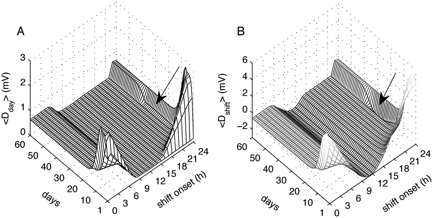
Average daily <D_day> (A) and shift <D_shift> (B) sleep drives depending on the shift onset and the number of days spent on the schedule. Arrows indicate the presence of long-lasting changes in average sleep drives for shifts starting around 2300 h. The <D_day> is calculated every day for the time interval between 0000 and 2400 h. The <D_shift> is calculated across the 8 hours of the shift.

The 8-hour shift schedules starting between 0800 and 1400 h, which are basically normal daytime work schedules, do not change sleepiness, with <D_day> and <D_shift> remaining the same irrespective of how many days are spent on the schedule. Figure 4A and 4B in addition show the number of days needed to achieve re-entrainment and the circadian phase response curve (PRC) for different shift onsets with Δϕ _C calculated from equation 2. It is easy to recognize these daytime shifts do not lead to re-entrainment of the circadian pacemaker, and the phase difference Δϕ _C is zero on these schedules. This happens because these shifts do not modify either light profile (shift light interval is inside the ambient light interval) or sleep-wake time (workers are awake anyhow during those hours, with sleep between 2330 and 0730 h).

Figure 4.

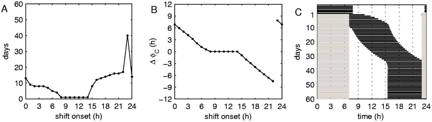
Entrainment of the circadian pacemaker to different shift schedules. (A) Dependence of the number of days needed for entrainment on shift onset. (B) Phase response curve (PRC) of the circadian pacemaker on the placement of the shifts at different times of the day. (C) Activity plot for the shift schedule with shifts starting at 2300 h. Black color indicates sleep intervals, and gray color indicates shift intervals. First day on the ordinate corresponds to the first day on the shift schedule.

Shifts starting between 1500 and 0700 h modify sleep-wake times and the light input by adding light and forced wakefulness either at the beginning or end of the ambient light interval and gating light during new sleep times. As Figure 3 demonstrates, these shifts initially result in an increase of <D_day> and <D_shift>, which happens due to an increased homeostatic pressure similar to the example in Figure 2. After this initial increase, sleepiness decreases due to circadian re-entrainment to the new light and wake schedule, which allows longer sleep during breaks and decreases H. The highest sleepiness during adaptation days is thus achieved on schedules that encompass circadian minimum (or D_max) within the shift. These schedules lead to high D during shifts and to low D during breaks, which results in shorter sleep time with consequent increase of H and <D_day>.

Although the evening (shift onset between 1500 and 2200 h) and night (2400-0700 h) shifts lead to qualitatively similar changes in sleepiness, they result in different changes of the circadian phase and entrainment time. The PRC in Figure 4B shows that night shifts lead to phase advance of the circadian pacemaker while evening shifts lead to its delay, which can be explained by well-known phase properties of the circadian pacemaker (Roenneberg et al., 2003; Golombek and Rosenstein, 2010; St. Hilaire et al., 2007). Entrainment to night shifts is achieved faster than to evening shifts, as seen in Figure 4A. This is a counterintuitive finding because it is known that night shifts are the worst in workers’ experience (Åkerstedt, 1995; Boivin et al., 2007; Dinges, 1995). We address this question in more detail below.

Changes of sleepiness on the shift schedule with shifts starting at 2300 h have different dynamics from the other schedules, as indicated with arrows in Figure 3. On this schedule, following a decrease of <D_day> and <D_shift>, they reach a minimum and start to increase again until the stable state is finally reached. This leads to a much longer entrainment time (Fig. 4A) and happens due to type 0 phase transition for this shift onset, as seen in the PRC in Figure 4B. Figure 4C demonstrates the activity plot for sleep and shift times on this schedule. Even though the re-entrained circadian phase is advanced compared to the initial one, it reaches this state via delay, as it cannot advance due to forced waking during the shifts preceding sleep. Hence, instead of covering the phase difference of 8 hours, it is forced to cover 16 hours. This also explains the minimums in <D_day> and <D_shift> for this shift around day 30 (Fig. 3). Unlike other shifts, re-entrainment to the 2300-h schedule leads to the circadian maximum passing through the shift interval. When circadian maximum (or D_min) is around the middle of the shift interval, the minimum in <D_shift> is achieved, with the values of <D_shift> on this day close to those on the optimal daytime schedules.

Finally, Figure 5A demonstrates the levels of <D_shift> and <D_day> when entrainment is achieved. As seen in Figure 5A, the night and evening schedules differ from each other in sleepiness values, but within the schedules, the shift onset time does not affect the resulting sleepiness; that is, <D_day> and <D_shift> are constant for different evening and night shifts. At the same time, <D_day> on the daytime shift is similar to that on the evening shifts, while <D_shift> is significantly different.

Figure 5.

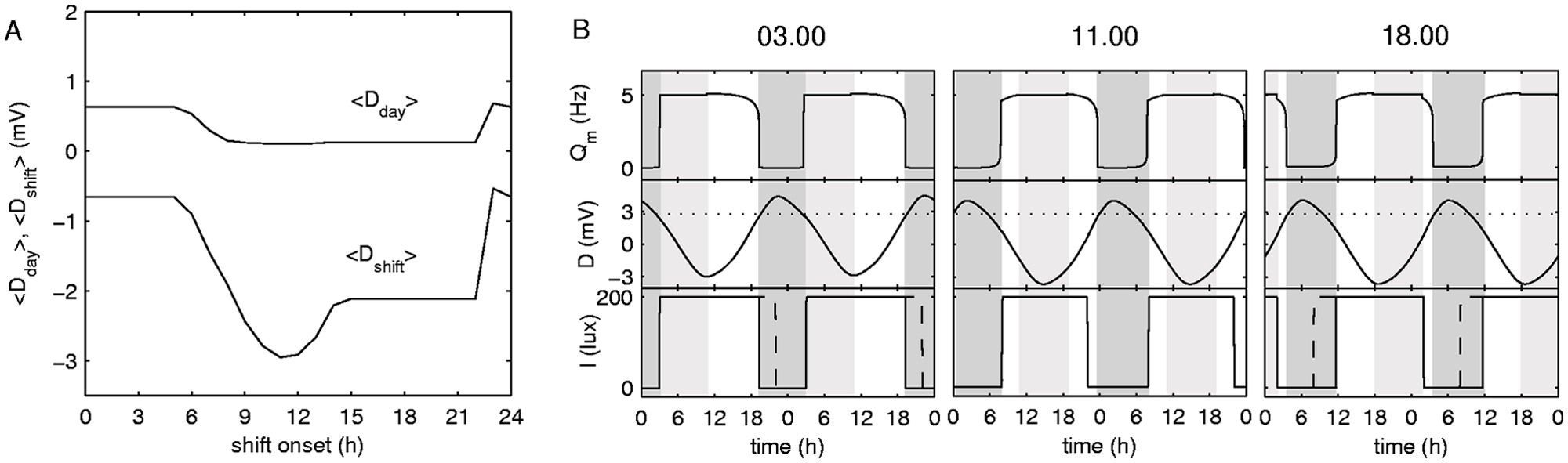
Sleepiness in the entrained system. (A) Dependence of the average daily <D_day> and shift <D_shift> sleepiness on shift onset in the entrained system. (B) Examples of time traces of the system entrained to the schedules with shifts starting at 0300, 1100, and 1800 h. Top panel shows the average firing rate of the wake-active MA neurons, middle panel demonstrates changes of sleepiness, and bottom panel shows the light profile (solid line = final; dashed line = initial). Dark shaded areas indicate sleep intervals, and light shaded areas indicate shift intervals.

Taken together (Figs. 4 and 5), a number of major questions appear that need to be answered to understand the dynamics. Below, we address these questions one after another and explain the mechanisms using the examples of activity on different schedules shown in Figure 5B.

Why do night shifts entrain faster than evening ones?

This is related to the longer photoperiod on night shifts than evening ones. As examples in Figure 5B demonstrate, night shift schedules have light during the entire wake period, while evening schedules have a certain period of darkness right before the transition to sleep. The figure demonstrates examples for 0300-h and 1800-h schedules, but a similar situation is observed on all night and evening shifts.

Why is the photoperiod on night schedules longer than on evening ones?

The duration of the photoperiod in the model is determined not only by the shifts and ambient light but also by the timing of sleep, which gates the light to 0 lux, and hence by the shape of D. Because we force wakefulness during the shifts on the night shifts, the starting time of the photoperiod is determined by the shift onset and the end time by the beginning of sleep. On the evening shifts, it is vice versa: the start of the photoperiod is determined by the end of sleep and the end by the end of the shift.

The circadian oscillator tends to entrain in such a way that C_max, and hence D_min, appears near the middle of the light interval, given that light intensity is constant on the interval. When entrainment is achieved, the wake time is normally about 16 hours, and because the shifts take about half the entire wake time (8 hours), the circadian maximum will always entrain to appear near the end of the night shift interval or beginning of the evening shift interval, as seen in Figure 5B for the examples of 0300-h and 1800-h shifts.

Sleep is induced when D reaches a threshold value, which is shown in Figure 5B with a dotted line. If the shape of D would be exactly sinusoidal, there might have been no difference between the lighting duration on night and evening shifts. However, the shape of D is slightly skewed, with a steeper rise than decay near the maximum. This leads to unequal duration of sleep on the rising and decaying parts of D, as can be recognized in Figure 5B. The values are about 3 hours on the rising part and about 4.5 hours on the decaying part for night schedules and 5.5 hours for evening schedules. On the evening shifts, the sleep on the decaying part continues even after D has decreased below the threshold value. This is explained by a bistability of sleep and wakefulness near the transitions, and because the system is not pushed away from the stable sleep branch, it stays on it until it becomes unstable (for details, see Fig. 3 in Phillips and Robinson [2007]).

The time intervals between C_max and C_min are about 12 hours. Thus, on the night schedules, the durations of sleep (4.5 hours) and the shift (8 hours) fully cover the decaying part of D, so that all the resting wake period appears during the rising part of D after the shift. Sleep on such schedules appears much earlier than ambient lighting would end, which results in lighting present during the entire wake period on these schedules. On the evening schedules, sleep and shift cover only 11 hours of the rising part. As D_min is located at the beginning of the shift interval, this will always result in about a 1-hour gap between shift and sleep during which there is no light present. Thus, the photoperiod on the evening shifts with the present setting of the model is always shorter than on the night shifts.

Why is <D_day> higher when the system is entrained to night schedules than to evening ones?

Sleep time in the system entrained to the night schedules is lower than when it is entrained to the evening ones, with 7 hours 30 minutes versus 8 hours 20 minutes. This results in generally higher H and D. The shorter sleep time is related to the fact that on the night schedules, wakefulness is forced by the shifts as soon as D crosses the threshold value, preventing sleep in the bistability region.

Why is <D_shift> higher when the system is entrained to night schedules than to evening ones?

This effect is determined by 2 factors. The first is the above-described higher daily sleepiness on the night schedules than on evening ones. However, it is easy to see from Figure 5A that the difference for <D_shift> is much bigger than for <D_day>. This additional difference is again explained by the skewed shape of D: near its minimum, the decaying part of D (night shifts) is steeper than the rising part (evening shifts). Hence, the area under the rising part of D is smaller than the area under the decaying part, giving the same relation for the average values on the 8-hour shift intervals.

How is the shape of <D_shift> in the system entrained to the daytime schedules explained?

Because daytime schedules do not re-entrain the circadian pacemaker, D_min appears at 1500 h on all of them. For the 1100-h schedule, this means that D_min is located right in the middle of the shift interval, which leads to the lowest area under the D curve during the shift and to the lowest mean value. When the shift starts earlier or later than 1100 h, the D_min will be located closer to either the beginning or end of the shift, which leads to higher <D_shift>.

Effects of Noise

In order to examine robustness of the obtained results, we have added white noise with uniform distribution in different variables of the model, including average potentials of the MA (V_m) and VLPO (V_v) neurons and light intensity (I). We have allowed noise intensity leading up to ±10% fluctuations of each variable’s range, for example, up to ±2.5 mV for V_m, which is changing between −22 mV and 3 mV. Noise with this intensity had almost no effect on the model’s dynamics. The resulting PRCs, entrained values of <D_day> and <D_shift>, and entrainment time (day_e) were the same as in the deterministic case in Figures 4 and 5. This shows that the obtained results are stable.

Effects of Weekends

The case of permanent shifts considered above is idealized in order to understand the underlying mechanisms. However, in practice, many of the parameters are changing, thereby affecting the dynamics of the system. For example, workers do not normally work every day for 2 months but have 2 days off after each 5 days of work. Figure 6 illustrates how addition of such weekends with a free schedule of sleep and wakefulness affects the sleepiness of workers and circadian entrainment to the shift schedule.

Figure 6.

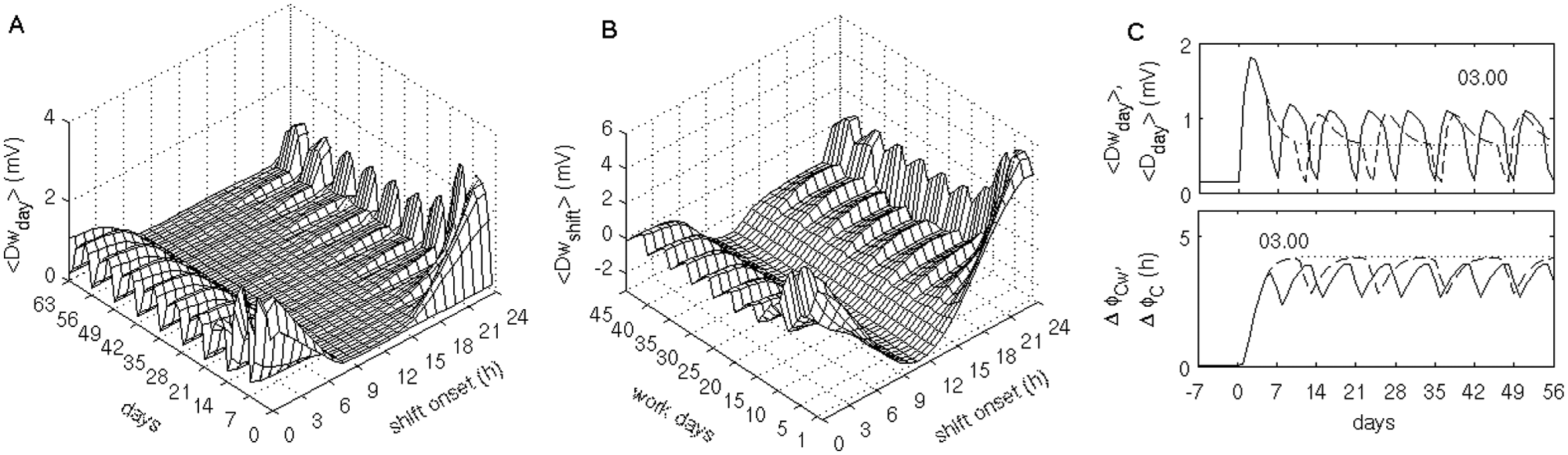
Average sleepiness on schedules with weekends depending on the shift onset and the number of days on the schedule. Mean daily sleepiness <D_day> taken across 24 hours (A), and mean sleepiness on the 8-hour shifts <D_shift> (B). (C) Plots demonstrate average sleepiness (top) and circadian phase difference (bottom) for the night schedule with shifts starting at 0300 h. Solid line indicates the results for schedules with 2 days off after 5 days of work; dashed line indicates the results for a schedule with 1 day off after 10 days of work, and dotted line indicates a permanent work schedule. Day counts start from the beginning of the shift schedule.

As can be seen from the maps of average sleepiness in Figure 6A and 6B and examples for <D_day> and Δϕ _C on the 0300-h schedules in Figure 6C, complete circadian entrainment is never achieved on either night or evening shifts in the presence of weekends. Sleepiness on such schedules increases during the work days, and before re-entrainment can be achieved, weekends interrupt it by introducing different zeitgebers and free sleep-wake activity. Sleepiness drops significantly during the weekends but increases again during work days. Entrainment during the work days can better be achieved on the schedules with shift onsets only slightly different from the normal daytime work starting between 0800 and 1400 h. On such schedules, sleepiness drops towards the end of the week, but weekends again disturb entrainment, and a first work day is associated with higher sleepiness.

The dashed line in Figure 5C demonstrates <D_day> and Δϕ _C for a 0300-h schedule with a different pattern of weekends: 1 day off after 10 days of work. Sleepiness on such a schedule is on average lower than on the previous schedule, and entrainment is achieved in the last days of work. However, it is again destroyed by the following day off. In this context, Figure 4A can also be interpreted as an indicator of the number of days for which it is essential for the worker to follow shift zeitgebers, also during the days off, in order to achieve entrainment to different schedules.

Discussion

In the present work, we have applied a previously developed physiologically based model of sleep and circadian entrainment to examine the effects of permanent shifts in schedules on sleepiness and re-entrainment. Multiple factors affect sleepiness of shift workers, so it is essential to not only make predictions about particular schedules but also most importantly to understand the underlying general mechanisms. The model used here can account for a large variety of factors, including complicated light profiles, variation of sleep-wake times, for example, due to social commitments, and any type of shifts and schedules of days off. Implementation of these diverse conditions would make the simulations closer to reality but at the same time would make it almost impossible to understand the mechanisms behind the dynamics. Therefore, in order to understand the complicated realistic schedules in the future, we have examined the simplest case with permanent shift schedules, weekends, and the simplest light profile with constant lighting intensity when light is present.

In good agreement with experimental data (Folkard and Åkerstedt, 2004), we have shown that sleepiness is increasing during the first days on all shift schedules besides the normal daytime work. This is related to increased homeostatic pressure due to insufficient sleep during active circadian phase. Studies with longer term effects of shift work show that the number of accidents on night shifts starts to decrease after the fifth night on the shift schedule (Folkard and Åkerstedt, 2004). Our simulations support these results, showing that sleepiness decreases when circadian phase changes sufficiently to allow longer sleep times. The degree of the initial increase of sleepiness on the schedule is associated with a shift of the circadian phase introduced by re-entrainment.

We have also found that the circadian phase curve in response to the considered shift conditions has type 0 phase transition for the shift starting around 2300 h (more precisely at 2224 h). The shifts that start shortly after the transition are the most difficult to entrain to and should be avoided. If shifts around that time are unavoidable, it is best to schedule them before the transitions or at least 1 or 2 hours after. Naturally, the timing of the phase transition will be different for different ambient and shift light conditions. Furthermore, other light settings may lead to a smoother, type 1 transition, which we expect to be easier in terms of entrainment. PRCs for specific shift schedules can be obtained experimentally and would prove highly useful for improving the design of shifts.

In practice, re-entrainment to shift schedules is not easy to achieve due to disturbances of sleep-wake cycles by social commitments, changes in lighting, or days off. Sometimes, circadian rhythms of workers can stay unentrained for many years (Folkard et al., 2005; Boivin et al., 2007), affecting their health and increasing chances of diseases (Knutsson, 2003). In agreement with this, we demonstrated that a common schedule with 2 days off after 5 days of work completely prevents entrainment and stabilization of sleepiness on the schedules with shift onsets between 1500 and 0700 h. Although it is well known that days off affect entrainment, these simulations highlight why it is critical to follow the same sleep-wake schedules on the days off as on work days. It is noteworthy that the time intervals determining daytime work, evening or night schedules, as described here, depend on the ambient light profile and will be different for workers exposed to different lighting. When the lighting during shifts is significantly different from that during breaks, the daytime work may also need re-entrainment during the first days on the schedule, leading to changes in sleepiness.

The present study creates a background for the examination of more complicated and realistic shift schedules and the development of measures helping to improve sleepiness and entrainment. In future studies, we will thus introduce forward and backward rotating shift schedules, examine how waking time affects sleepiness during the shift, and study how lighting can be adjusted to improve entrainment and sleepiness. Other measures should also be probed to help estimation of the effectiveness of a shift schedule. These include “performance”, which should also account for sleep inertia (McCauley et al., 2009), or “wake effort”, which is based on the stimulus level required to keep the stability of the wake state (Fulcher et al., 2010). In the present study, we have also assumed that light during sleep is gated to zero. In practice, this is true for some situations, while in others, some light may still penetrate eyelids during sleep and affect circadian re-entrainment (Dumont et al., 2001). This should also be taken into account in the future studies, along with examination of how photic and nonphotic inputs individually entrain the circadian pacemaker.

Overall, the structure of the model allows easy implementation and study of specific experimental protocols, which should be done in the future for further validation of the model and aid in explaining experimental observations and the design of more efficient protocols. Potentially, this model can also be used to make individual predictions regarding most appropriate shift schedules and conditions.