Sage Journals: Discover world-class research

Abstract

Spanish

Chinese

Empirical research on the impact of congestion on travel behavior remains limited. This study fills this gap using a comprehensive analytical framework, an improved time-related travel delay measure, structure equation modeling, and the disaggregated household survey data for the Puget Sound Region. The results indicate that travel time delay is associated with fewer household vehicles, fewer vehicle trips, and lower vehicle miles traveled. The findings confirm the intricate impacts of the travel time delay, reinforce the importance of the “D” factors in travel behavior, and point to the need for comprehensive solutions to travel demand management.

Keywords

travel time delay congestion built environment travel behavior structure equation model

Introduction

Traffic congestion is a major concern of planners, economists, environmentalists, individuals, and households, as it has grown considerably in cities of every size and affected urban structure, the spatial distribution of urban activities, economic productivity, and environmental quality of cities, as well as the daily life of individuals and households (Downs 2004; Schrank et al. 2021). Reducing traffic congestion has become a significant goal in the realm of transportation policy and planning. While differing in approach to traffic congestion, land use policies, such as compact development, transit-oriented development (TOD), urban infill, and the like, and toll/congestion pricing policies have been proposed or used as tools to reduce or contain traffic congestion (Ewing and Bartholomew 2018; Ewing, Tian, and Lyons 2018; Gordon and Lee 2015).

Land use policies are mainly based on findings from studies of travel behavior impact of the built environment. Common measurements of the built environment and urban form are the “5D” factors, such as density, diversity, design, destination accessibility, and distance to transit (Stevens 2017). It has been argued that higher land use density and diversity in neighborhoods, better design to increase access to destinations, and shorter distance to transit services can increase the propensity of nonautomobile travel and reduce the necessity of driving, therefore reducing vehicle miles traveled (VMT) (Cervero and Kockelman 1997; Ewing and Cervero 2001; Ewing, Tian, and Lyons 2018; Lamíquiz and López-Domínguez 2015; Zahabi et al. 2015). In addition, some scholars further suggest that traffic congestion, which may be a result of high-density developments as some critics of land use policies have argued, may reduce VMT because commuters may change their travel behavior to avoid traffic congestion (Ben-Akiva and Lerman 1985; Sarzynski et al. 2006). Despite the argument, fewer empirical studies have investigated the effect of traffic congestion on travel behavior (Sardari, Hamidi, and Pouladi 2018).

This study addresses the aforesaid gap by investigating the effect of travel time delay on travel behavior in terms of VMT per household. This study finds evidence of traffic congestion effects. It contributes to the literature by empirically testing a theory that has been proposed but not fully demonstrated. This research also adds to the current studies by considering self-selection factors in addition to household socioeconomic and neighborhood built environment characteristics and operatizing the conceptual framework via structural equation modeling (SEM). Moreover, the delay score created in this study can distinguish congestion from nonsaturated traffic condition, a shortcoming of the widely used volume/capacity ratio as a measure of traffic congestion. In the following sections, we first provide a brief review of the existing travel behavior studies and discuss the relationships among urban structure, travel behavior, and traffic congestion. Following the description of the research methodology, we present the model results. The final section summarizes the research findings, discusses implications of the findings and limitations of the study, and offers suggestions for future research.

Urban Structure, Travel Behavior, and Traffic Congestion

The relationship between the built environment and travel behavior has been a subject of numerous studies. Consideration of the interaction between land use patterns and travel behavior can be traced to the work of Mitchell and Rapkin (1954), which theorizes how and why people and freight move; why traffic occurs; and what the interrelations among transportation networks, passenger and goods movements, land use design, and distribution of activities are. The work of Mitchell and Rapkin (1954) lays the groundwork for studies of factors contributing to travel behavior (Beaver 1956; Wallace 1956).

The Effects of the “D” Factors

Building upon the work of Mitchell and Rapkin (1954), a large body of research has focused on the effects of built environment on travel behavior. For instance, having tested the effects of density, land use diversity, and pedestrian-friendly design (commonly known as the 3D’s) on household vehicle miles of travel and mode choice for nonwork trips, Cervero and Kockelman (1997) concluded that an increase in each of the 3D’s is associated with a modest or moderate decrease in travel demand. Later studies have extended the 3D’s to include the effects of other D’s such as demographic factors, distance to transit, destination accessibility, demand management, density and quality of transit services, and so on (Christiansen et al. 2017; Ewing and Cervero 2010; Guerra et al. 2018; Majid, Nordin, and Medugu 2014).

Conventional wisdom about the impacts of land use and urban form on travel behavior perceives suburbanization of low-density development as the stimulating engine of increasing traffic congestion (Downs 1992; Gillham 2002; Sarzynski et al. 2006). It has been argued that low-density housing and the separation of residential and workplace locations, a circumstance known as job–housing imbalance, among others, encourage longer commutes with higher vehicle usage and trip frequencies, resulting in more commute time and higher levels of traffic congestion. Studies have also argued that diverse population, better accessibility to transit and destinations, higher quality of transit services, and incentive for carpooling and transit subsidy would discourage vehicle travel. Researchers along this line of inquiry typically propose high-density, compact, and mixed development policies to reduce traffic congestion (Cervero 1989, 1996; Downs 1992; Ewing 1994, 1997; Ewing, Deanna, and Li 1996; Ewing, Pendall, and Chen 2003).

Critics of land use policies recognize the short-term effect of land use on travel behavior and traffic congestion but offer a countering argument for the long-term effect of suburbanization. For instance, Gordon and Richardson (1997) argued that while traffic congestion is inevitable due to short-term disequilibria, suburbanization in the long run would result in shorter trips, lower VMT, and higher average speed, which leads to lower levels of traffic congestion as a result of market self-correction. They supported this argument with statistics of changes in commute time from national household surveys, as well as results from other studies (e.g., Gordon, Richardson, and Jun, 1991; Levinson and Kumar 1997). Later studies also provide some support for the argument with cautions. For example, Crane and Chatman (2003) used the American Housing Survey data between 1985 and 1997 at the Metropolitan Statistical Areas (MSA) level and the two-stage least squares regression model for analysis. They found that more decentralization of jobs to suburban areas is associated with shorter commute distance on average after controlling for wage, land costs, and other factors. However, there was a large difference in commute distance by industries. Some industries, such as construction, wholesale, and retails, followed population decentralization and displayed shorter commute distance. Other industries, such as manufactory and finance, were found to associate with longer commute distance. Holcombe and Williams (2010) investigated the relationship between sprawl and commute time using the microdata of the 2001 National Household Travel Survey (NHTS) and the multilevel modeling technique. The results indicated that shorter commute time was associated with decentralization of employment. Holcombe and Williams (2010), however, were cautious about the implication of the results, as the model explained less than 5 percent of the variance in individual private vehicle commute time. Using data for seventy-nine large MSAs in the United States from the 2000 census, the American Community Survey (ACS) 2005–2009, and the NHTS of 2001 and 2009, Gordon and Lee (2015) compared changes over time, modeled the effects of urban spatial structure measured by population density, a decentralization factor along with other covariates, and concluded that the average commute time remained stable despite population growth. They attributed the phenomenon to urban suburbanization.

The Influence of Self-Selected Factors

Quite a few researchers have argued that research on travel behavior is incomplete without considering self-selection factors, defined by Van Wee (2009) as conscious decisions about travel and/or residential locations based on their abilities, needs, and preferences (see, for example, Cao, Mokhtarian, and Handy 2009 and many more). Van Acker, Mokhtarian, and Witlox (2011) demonstrated the difference in model outcomes between including and ignoring subjective attitude variables in mode choice modeling. Many studies also provided evidence about the mismatch between preferred and actual residential locations (Badland et al. 2012; Bagley and Mokhtarian 2002; Bohte, Maat, and van Wee 2007; Cao, Mokhtarian, and Handy 2009; De Vos et al. 2012; Frank et al. 2007; Kamruzzaman et al. 2013; Olaru, Smith, and Taplin 2011), as well as the heterogeneity among individual households’ response to a given built environment (Cao and Chatman 2015). Li (2018) conducted in-depth focus group interviews in three TODs in Dallas/Fort Worth metroplex. She found that social belonging and access to diverse amenities are key factors for residential decisions. While proximity to transit is valued in residential decisions, actual travel modes may be inconsistent with travel preference, due to other limitations. Næss et al. (2019) studied the effects of built environment on travel with the control of residential location self-selection factors in the Oslo and Stavanger areas. Travel behavior is measured by trip distance and mode share for both commute and nonwork activities. The authors used both cross-sectional and longitudinal designs for their analysis and triangulated the results with those from the qualitative analysis of in-depth interviews. The authors concluded that after controlling for self-selection factors, higher population density within the local area of residence is associated with lower car use but not with travel distance. Distance between residential location and city center tends to play a role in car use. Specifically, those who live closer to city center tend to make fewer car trips than those who live far away. Land use diversity is associated with shorter travel distance only if land use mix has reached a level of critical mass. In particular, a better match of job skills and job opportunities is required for shorter commute distance. Moreover, the local street pattern, a measure of the design factor, is found to be an insignificant factor in travel decision.

Traffic Congestion on Travel Behavior: A Reversed Impact?

The foregoing discussion reveals that travel behavior is complex, and more empirical studies are needed. The discussion also shows that the current literature has largely focused on the effects of land use, urban form, and built environment on travel behavior or traffic congestion, with the control of demographic and self-selection factors. None of the aforesaid studies considers the effect of traffic congestion on travel behavior. More than thirty years ago, Ben-Akiva and Lerman (1985) hypothesized that traffic congestion provides negative feedback to transportation systems by increasing travel time and travel costs. Due to the negative impacts of travel time delay, commuters may change their residential location and/or travel behavior to maximize benefits and save time by avoiding traffic congestion, which could be in the forms of making more short-distance trips, reducing vehicle miles of travel, substituting automobile trips with nonautomobile trips, eliminating travel, changing time or/and route of travel, or changing trip destinations. Inexplicitly, scholars who question the effectiveness of land use policies seem to suggest that traffic congestion may affect residential location decision and/or travel behavior. However, these hypotheses had not been empirically tested until recent years, though the contemporary results are misty. For example, Salon (2009) investigated the effect of population density and travel costs, including travel time, subway availability near home, and parking availability and costs, on car use for commute trips. Using multinomial logit modeling, she analyzed the survey data of New York City in 1997–1998 and found that the likelihood of car use would decrease if the costs of driving increase. Her finding implied the effect of traffic congestion on travel mode choice as hypothesized by Ben-Akiva and Lerman (1985). However, due to the lack of traffic congestion data, the study was unable to test the effect of traffic congestion on car use for commute trips.

Mondschein and Taylor (2017) examined the effects of traffic congestion on trip frequency, driving, and walking using the Southern California Association of Governments (SCAG) household travel survey data for metropolitan Los Angeles and negative binomial regression and logistic regression models. Local traffic congestion in their models was measured by the volume and capacity (V/C) ratio during peak hours. Besides individual travelers’ sociodemographic factors, their models included a few land use variables such as categorical variables of activity density and job location, defined as working at home or in many locations. Their results did not show a particular pattern, as traffic congestion was found to be in places with either low or high densities. They concluded that traffic congestion could coexist with trip making and activity participation in some places regardless of density. According to them, more people gathering in one place at the same time are likely to create traffic congestion; however, traffic congestion may not avert trip making and activity participation if there exist multiple travel options and agglomeration of economic activities.

Using disaggregated data from the 2009 NHTS and structure equation modeling, Sardari, Hamidi, and Pouladi (2018) found an inverse relationship between VMT and traffic congestion around individuals’ home locations. Similar to Mondschein and Taylor (2017), they used household travel data for all trips and measured traffic congestion by the V/C ratio using the annual average daily traffic (AADT) data. While popular, such a congestion measure is misleadingly simplistic as it does not catch the nature of traffic congestion and cannot distinguish between saturated and nonsaturated traffic conditions. In addition, they controlled for some land use and sociodemographic factors, though the specific measurements may not be the same as the ones by Mondschein and Taylor (2017). Both studies did not control for the effects of self-section factors on travel.

In short, the review indicates that empirical research on the effect of traffic congestion on travel behavior is in its infancy. Results of the limited studies are mixed. In addition, the limited studies of the congestion effects on travel behavior did not control for self-selection factors. Moreover, the V/C ratio used in the current literature as a measure of traffic congestion does not differentiate the saturated and nonsaturated traffic conditions. Despite the limitations, the aforementioned studies are a few pioneers in empirically testing the impact of traffic congestion on travel behavior. They point to a forgotten area that deserves attention in research and demonstrate the needs for further investigation of the effect.

Method

This research builds upon previous studies on the effects of traffic congestion and tests a theory that has been proposed but not yet fully investigated before. It adopts an improved framework for the investigation by including self-selection factors in addition to common factors considered in the prior studies. Moreover, it uses an improved time-related travel delay measure and implements SEM, an advanced statistical technique appropriate for the study. In the following, we first lay out the conceptual framework and hypotheses. Then, we explain the data used for this study, their sources, and data-processing approach.

Conceptual Model and Research Hypotheses

Travel behavior can be measured in terms of person miles traveled (PMT), household VMT, travel mode, travel time, route choice, or trip frequency. These dimensional measurements are interrelated. For example, nonautomobile travel modes, such as walking, biking, or transit, are often associated with shorter distance or longer travel time for the same distance than automobile travel. In addition, more short-distance trips and nonautomobile travel may be a substitute for automobile trips, and hence may reduce VMT. In this study, we focus on the effect of traffic congestion on VMT, while controlling for, to the extent allowed by the data, work location, trip frequency, and other pertinent factors as suggested by the existing literature. The unit of analysis in this study is household.

Figure 1 illustrates the framework for investigating the effect of traffic congestion on travel behavior with the control of factors in three broad categories including household demographic and socioeconomic characteristics, land use and built environment factors, and self-selection factors. These factors affect travel outcome directly and indirectly through mediating factors, which in this model include number of trips and household vehicles.

Figure 1.

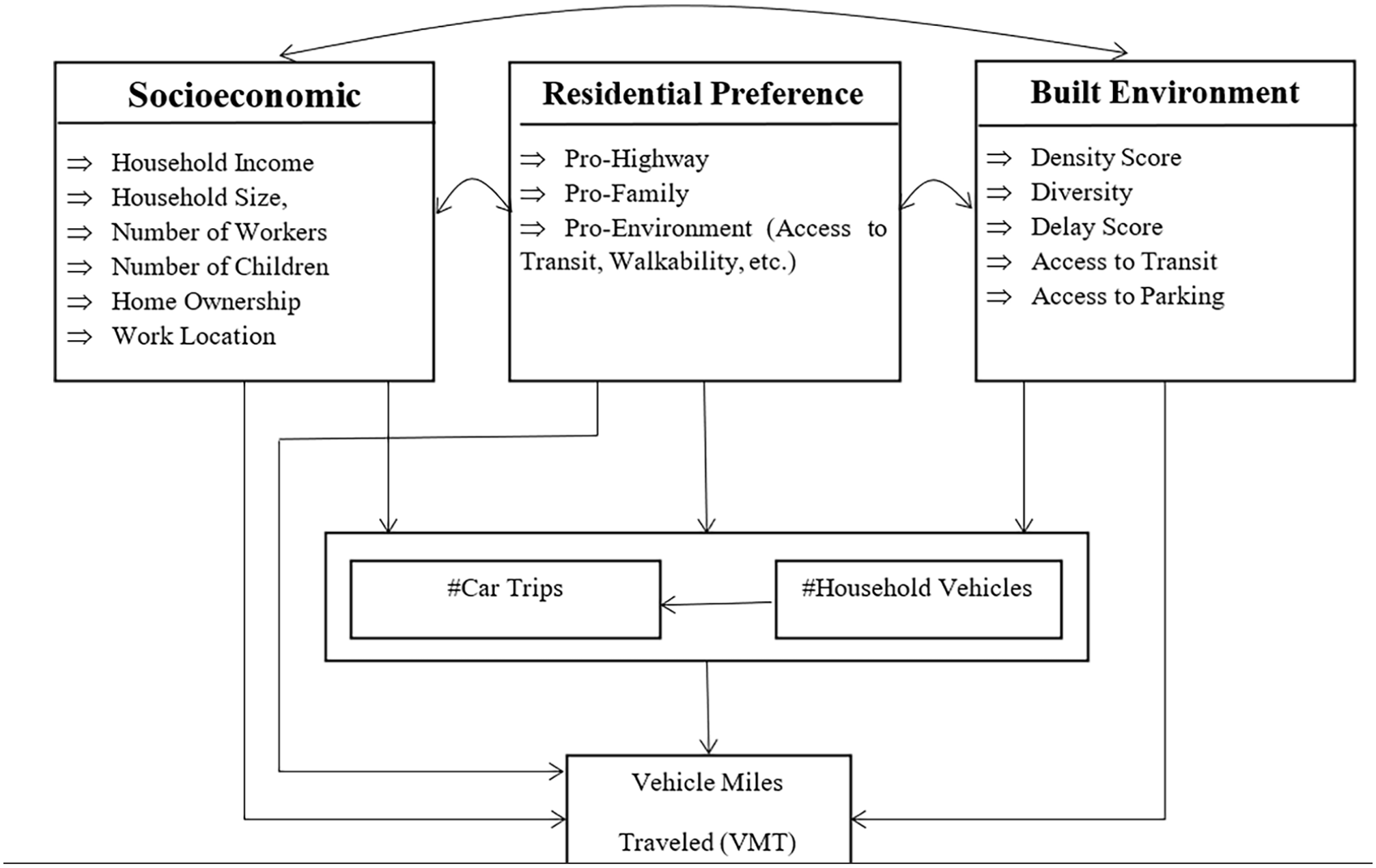
Effects of traffic congestion.

We propose the following hypotheses for testing:

As indicated by the single-headed path from household characteristics to VMT in Figure 1, household characteristics directly influence VMT. Specifically, higher household income increases VMT because households with a higher income tend to own more vehicles and make more household vehicle trips, which will lead to higher household VMT. Larger households, more workers in the household, and more children will be positively associated with VMT. Homeowners are more likely to have higher VMT than nonhomeowners. Households with members working at home tend to have lower VMT than households with members not working at home. As displayed by the two single-headed paths in Figure 1, household characteristics also indirectly affect VMT via household vehicle count and household vehicle trip. The double-headed curves linking household characteristics with self-selection factors and built environment indicate household characteristics are correlated with the self-selection factors and the built environment factors.

In the same vein, the self-selection factors, as hypothesized in the previous studies by Cao, Mokhtarian, and Handy (2009) and others, directly influence VMT and indirectly impact VMT through vehicle trip and household vehicle count, and they are also correlated with household characteristics and the built environment factors.

The D factors, representing the current land use and built environment, directly and indirectly through household vehicle trips and household vehicles affect VMT as suggested by Cervero and Kockelman (1997), Ewing and Cervero (2001, 2010), and many others. They are also correlated with household characteristics and self-selection factors. Traffic congestion measured by delay score, which is included in the land use/built environment category, may be inversely associated with VMT, household vehicles, and travel decisions as hypothesized originally by Ben-Akiva and Lerman (1985).

We tested this conceptual framework using SEM, a powerful statistical technique that sets itself apart from many traditional statistical techniques as highlighted by a number of scholars. Particularly, SEM is flexible as it can integrate multiple statistical tools such as equations, path diagrams, and matrices into a single framework that is appropriate for analyzing factors that are generally correlated with one another (Wang and Wang 2012). It can “incorporate both observed and unobserved variables” and “provides explicit estimates of these error variance parameters that many other statistical techniques ignore” (Bryne 2011). In addition, SEM allows for estimation of direct and indirect effects (Byrne 2012; Wang and Wang 2012). “By demanding that the pattern of intervariable relations be specified a priori, SEM lends itself well to the analysis of data for inferential purposes” (Byrne 2012). Figure 2 shows the diagram of the SEM. The predictors in each of the three categories and their hypothesized relationships are listed in Table 1.

Figure 2.

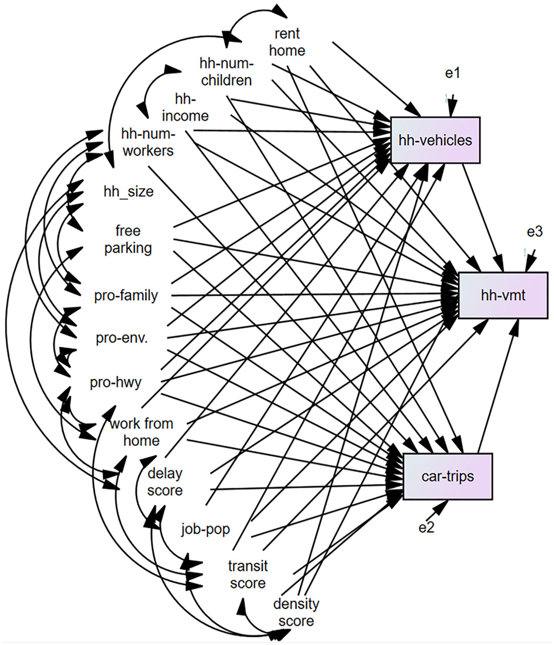
Causal path diagram explaining VMT per household.

Table 1.

Explanatory Variables and Hypothesized Relationships.

Predictors	Description/Definition	Relationship to exogenous factors	Relationship to mediating factors	Relationship to HH VMT
Household characteristics
hh_size	Household size	− home-rent + hh-child	+ hh-vehicle + car trips	+
hh_workers	Number of household workers	+ hh-size + hh-income	+ hh-vehicle + car trips	+
hh_child	Number of children in household	+ pro-family + hh-size	+hh-vehicle + car trips	+
hh_income	Household income	+ hh-workers − home-rent	+ hh-vehicle + car trips	+
home-rent	Living in rental homes (rent = 1; else = 0)	− hh-income − hh-size	− hh-vehicle − car trips	−
work-loc	Work location (home = 1; else = 0)	+ hh-income	− hh-vehicle − car trips	−
Self-selection factors for residential location
pro-hwy	Based on access to highway	+ free-parking + hh-income	+ hh-vehicle + car trips	+
pro-env	Based on access to public transit, walkability, or 30-minute travel time to work	+ transit-score + density-score + job/pop-score	− hh-vehicle − car trips	−
pro-family	Based on school, HH changes, close to friends and families.	+ hh-size + hh-child	+ hh-vehicle + car trips	+
Built environment factors
free-parking	No. of HH members with free parking at workplace	+ hh_workers	+ hh-vehicle + car trips	+
density-score	A factor of population, employment, road, and intersection densities	− hh-size + hh-rent − hh-income + transit-score	− hh-vehicle − car trips	−
Job/pop-score	Job/Population balance	+ density-score	− hh-vehicle − car trips	−
transit-score	No. of public transit routes	− hh-income − hh-size + hh-rent	− hh-vehicle − car trips	−
delay-score	Travel time delay	+ density-score − job/pop-score	− hh-vehicle − car trips	−
Mediating variables
hh-vehicles	No. of vehicles in an HH		+ car trips	+
car-trips	No. of car trips in an HH		+ hh-vehicles	+

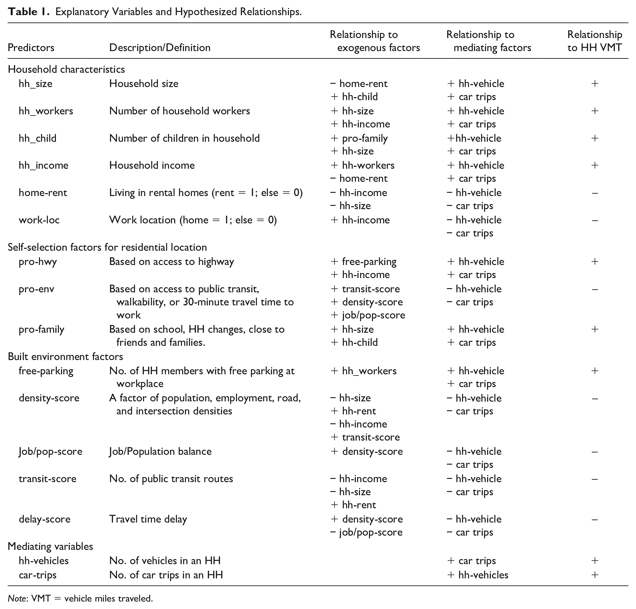
Note: VMT = vehicle miles traveled.

Data, Variables, and Measurements

The main data for this study come from the disaggregated 2015 household travel survey data from the Puget Sound Regional Council (PSRC) area. The PSRC travel survey data were selected primarily for two reasons. First, it was the most recent household travel survey data available at the time when this study commenced. Second, it was the first disaggregated travel survey dataset that includes the geocoded location of home, workplace, and all other trip-end locations. The 2015 PSRC travel survey dataset includes completed data for 4,786 persons from 2,442 households, with over eighteen thousand records of daily trips made by the survey respondents. All household socioeconomic variables, self-selection variables, and the free parking variable (an indicator of built environment) were extracted from the PSRC travel survey data.

Additional data were gathered from the 2015 NHTS, the U.S. Census, the Longitudinal Employer-Household Dynamics (LEHD) program, the TOD database, and the National Historical Geographic Information System (NHGIS). The GIS geospatial analysis tools and ArcGIS Modelbuilder were used to extract the built environment variables. Sardari, Hamidi, and Pouladi (2018) discussed the trade-offs between data intensity and research effect and recommended two-mile buffer from residential locations as the optimal thresholds to examine the interrelationships among land use patterns, traffic congestion, and auto usage. According to NHTS 2017, out of the travel day vehicle trips, 16.6 percent were commute trips, 34.3 percent were home trips, and 49.1 percent were related to shopping, social, medical, school, and other trips (Federal Highway Administration [FHWA] 2017). For these reasons, we decided to focus on traffic condition around residential locations and used the traffic congestion and built environment data in the two-mile buffer zones from individual households’ home locations.

The travel time delay score was an improved time-related travel delay measure for traffic congestion. It was calculated using time-related data from the Google Maps API. In this application, Google travel time data for a distance of two-miles around home locations were obtained for peak and off-peak hours during weekdays. Then, the delay score around each home location was calculated based on average speed during peak and off-peak hours within the two-mile network buffer. It is important to note that Google travel time data are based on historical data that are not allocated to a specific year. Google’s traffic model returns driving duration considering time spent in traffic, which is predicted based on historical averages (Google LLC 2018). Therefore, integrating these historical data into the household travel survey data provides an ideal travel time indicator. Equation (1) presents the formula for calculating the delay score. This delay measure overcomes the inability of the V/C ratio in differentiating traffic congestion under the saturated and nonsaturated conditions, normalizes the delay score, and therefore better reflects the local traffic condition without encumbering data collection and processing requirements.

Delay score = (1 - \frac{Average free flow travel time (weekdays)}{Average travel time during peak periods (weekdays)}) * 100 .

(1)

In addition, “home-rent” and “work-location” in Table 1 are dummy variables, in which living in rent homes and having an option of working at home, respectively, were coded as 1, and all else as 0. Moreover, the “pro-highway” variable was a five-point Likert-type scale from the 2015 PSRC travel survey dataset for the following question: “How important were each of these factors when choosing to move to where you live now (the residence where we sent your invitation to participate in this study)?—Being close to the highway.” Other self-selection variables were created using principal components analysis (PCA) based on responses to the relevant choices for the same question in the 2015 PSRC travel survey dataset (PSRC 2015). The factor loadings of these variables along with the testing statistics are described in Table 2. All the components have an eigenvalue, which measures the total amount of variance explained by a given principal component, greater than 1 and the explained variance greater than 76 percent. The values of the Kaiser–Meyer–Olkin (KMO) test, a measure to assess sampling adequacy of the data, are higher than the threshold of 0.6. Similarly, the results of Cronbach’s alpha test indicate that all factors have high internal reliability as Cronbach’s alpha values varied from .84 to .91, and all are greater than the threshold of 0.6.¹

Table 2.

Self-Selection Variables Extracted by PCA with Associated Statistics.

Variable	Factor loading	Factor	Eigenvalue > 1	Explained variance (%)	KMO (>0.6)	Cronbach’salpha (>0.6)
Employment density	0.846	Density factor	3.7	92	0.798	.890
Population density	0.922
Road density	0.966
Intersection density	0.955
Having a walkable neighborhood	0.854	Pro-environment	2.3	76	0.729	.838
Being close to public transit	0.888
Within a 30-minute commute to work	0.869
Quality of schools	0.867	Pro-family	2.5	85	0.715	.905
A change in family size or marital/partner status	0.955
Being close to family or friends	0.946

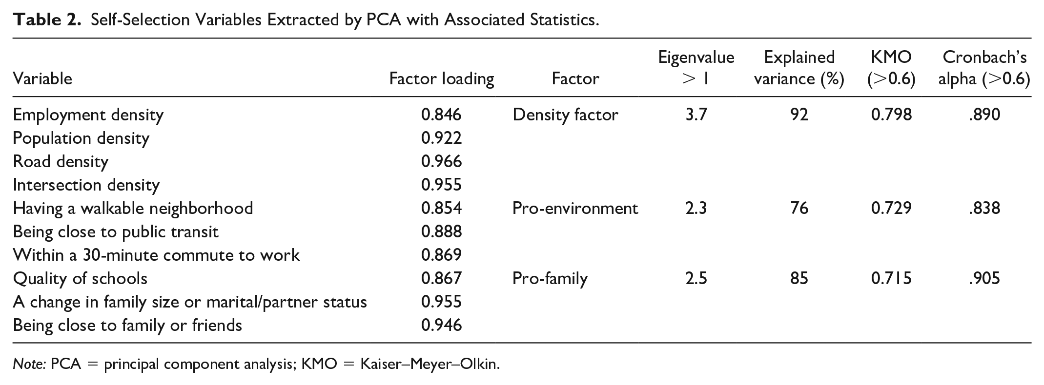
Note: PCA = principal component analysis; KMO = Kaiser–Meyer–Olkin.

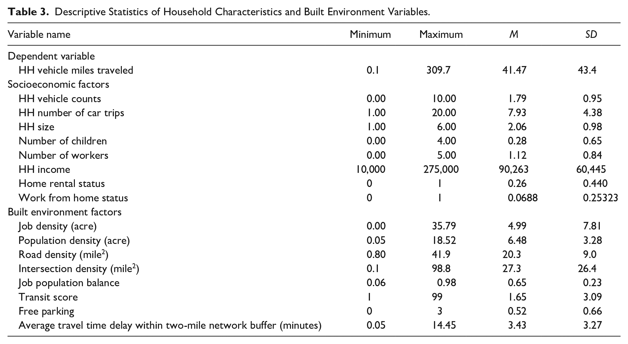
Except for “home-rent” and “work-loc,” other variables in Table 1 are continuous variables. These were transformed by taking natural logarithms to reduce the impact of outliers and provide parameter estimates as elasticities. The variable of “home-rent” indicates housing tenure status. Other household characteristics are not differentiated by tenure status. The descriptive statistics of all the variables, except for the self-selection variables reported in Table 2, are displayed in Table 3.

Table 3.

Descriptive Statistics of Household Characteristics and Built Environment Variables.

Variable name	Minimum	Maximum	M	SD
Dependent variable
HH vehicle miles traveled	0.1	309.7	41.47	43.4
Socioeconomic factors
HH vehicle counts	0.00	10.00	1.79	0.95
HH number of car trips	1.00	20.00	7.93	4.38
HH size	1.00	6.00	2.06	0.98
Number of children	0.00	4.00	0.28	0.65
Number of workers	0.00	5.00	1.12	0.84
HH income	10,000	275,000	90,263	60,445
Home rental status	0	1	0.26	0.440
Work from home status	0	1	0.0688	0.25323
Built environment factors
Job density (acre)	0.00	35.79	4.99	7.81
Population density (acre)	0.05	18.52	6.48	3.28
Road density (mile²)	0.80	41.9	20.3	9.0
Intersection density (mile²)	0.1	98.8	27.3	26.4
Job population balance	0.06	0.98	0.65	0.23
Transit score	1	99	1.65	3.09
Free parking	0	3	0.52	0.66
Average travel time delay within two-mile network buffer (minutes)	0.05	14.45	3.43	3.27

Results

We tested two models: one without the control of work location and vehicle trip variables (model 1) and one with the control of the two variables (model 2). The model fit statistics and maximum likelihood estimates of the model parameters are provided in the section below. The unstandardized and standardized coefficients of the regressors in the analysis are reported in the section following model fit statistics. Finally, we compared the importance of the regressors based on the standardized estimates. The unstandardized coefficients reflect the expected (linear) change in the outcome variable associated with each unit change in the regressor, while the standardized coefficients allow the comparison of relative strengths of the predictors on a common scale (Bollen 1989; Grace et al. 2018). With some exceptions, the results indicate that each direct effect is statistically significant at the .05 level or better. The main finding is that the level of traffic congestion, measured by delay score, is a significant predictor of household VMT. The following sections discuss the findings in further detail.

Model Fit Statistics

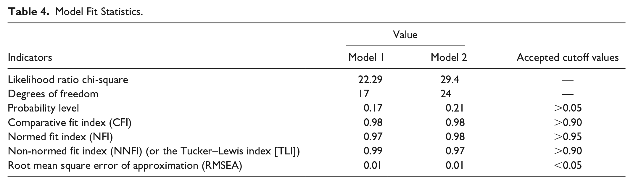
There are different indices for evaluating an SEM model’s goodness-of-fit. The traditional measure is the likelihood ratio chi-square test, which assesses the overall model fit and the discrepancy between the sample and fitted covariance matrices. The null model for the test is that model fits the data perfectly. According to Hox and Bechger (2007), a chi-square with a nonsignificant p value (>.05) indicates a good model fit. As seen in Table 4, the likelihood ratio chi-square is 22.29 for model 1 and 29.4 for model 2 with the significance levels at .17 and .21, respectively. Both are insignificant at the .05 level. The results suggest that both models fit the data well. However, the likelihood ratio chi-square statistics are sensitive to sample size. To further examine the model fit, additional goodness-of-fit indices were calculated. As indicated in Table 4, the comparative fit index (CFI), normed fit index (NFI), and non-normed fit index (NNFI) values are greater than the accepted cutoff value of 0.90. The root mean square error of approximation (RMSEA) values are smaller than the cutoff value of 0.05. The results confirm that both models represent a good fit to the data. Since model 2 controls for the effects of travel mode and work location, and is more comprehensive than model 1, we focus on the results of model 2.

Table 4.

Model Fit Statistics.

Indicators	Value		Accepted cutoff values
Indicators	Model 1	Model 2	Accepted cutoff values
Likelihood ratio chi-square	22.29	29.4	—
Degrees of freedom	17	24	—
Probability level	0.17	0.21	>0.05
Comparative fit index (CFI)	0.98	0.98	>0.90
Normed fit index (NFI)	0.97	0.98	>0.95
Non-normed fit index (NNFI) (or the Tucker–Lewis index [TLI])	0.99	0.97	>0.90
Root mean square error of approximation (RMSEA)	0.01	0.01	<0.05

In the following, we report the results by the effects on household vehicle counts, number of car trips, and VMT. We further detail the findings under each section along the dimensions of household socioeconomic characteristics, self-selection factors, and the built environment features, respectively. We close each section with the interpretations of standardized estimates.

Household Vehicle Counts

Table 5 shows the standardized and unstandardized parameter estimates for the direct effects of the predictors on the endogenous variables (i.e., household vehicle counts, household vehicle trips, and VMT) with single-headed arrows pointing toward them. With the log-transformation of the outcome variable, an unstandardized coefficient multiplied by one hundred can be interpreted as percentage change in the outcome variable for a one-unit change in the predictor variable. It is evident from Table 5 that all variables, except for the pro-family factor, are significantly and directly associated with household vehicle counts.

Table 5.

Maximum Likelihood Estimates for Direct Effects of Predictors on Household Vehicle Counts, Car Trips, and Vehicle Miles Traveled.

Variables	Standardized estimate (β)	Unstandardized estimate (B)	SE
Effects on household vehicle counts
Socioeconomic factors
hh-vehicles ← hh-size	.363***	0.368***	0.027
hh-vehicles ← hh-income	.141***	0.091***	0.013
hh-vehicles ← home-rent	−.132***	−0.143***	0.021
hh-vehicles ← hh-child	−.119***	−0.266***	0.047
hh-vehicles ← hh-workers	.09***	0.12***	0.03
hh-vehicles ← work from home	−.03*	−0.055*	0.033
Self-selection factors
hh-vehicles ← pro-environment	−.123***	−0.075***	0.013
hh-vehicles ← pro-highway	.05**	0.028**	0.011
hh-vehicles ← pro-family	.027	0.06	0.043
Built environment factors
hh-vehicles ← density-score	−.152***	−0.091***	0.015
hh-vehicles ← transit-score	−.114***	−0.017***	0.003
hh-vehicles ← delay-score	−.10***	−0.10***	0.025
hh-vehicles ← job/pop-score	−.088***	−0.086***	0.018
hh-vehicles ← free-parking	.071***	0.049***	0.014
Effects on household car trips
Socioeconomic factors
car_trips ← hh-size	.423***	0.585***	0.035
car_trips ← work at home	−.234***	−0.588***	0.041
car_trips ← hh-child	−.04	−0.04	0.06
car_trips ← home-rent	−.024	−0.036	0.026
car_trips ← hh-vehicles	.018	0.024	0.03
car_trips ← hh-income	.01	0.01	0.017
car_trips ← hh-workers	−.008	−0.014	0.038
Self-selection factors
car_trips ← pro-highway	−.036	−0.028	0.013
car_trips ← pro-family	.025	0.076	0.054
car_trips ← pro-environment	−.017	−0.014	0.016
Built environment factors
car_trips ← transit-score	−.601***	−0.126***	0.004
car_trips ← delay-score	−.118***	−0.163***	0.031
car_trips ← density-score	−.067*	−0.055**	0.019
car_trips ← job/pop-score	.044***	0.059***	0.022
car_trips ← free-parking	.024	0.022	0.018
Effects on household miles traveled
Socioeconomic factors
hh-vmt ← car_trips	.21***	0.959***	0.061
hh-vmt ← hh-workers	−.041	−0.343	0.096
hh-vmt ← hh-vehicles	.04***	0.246***	0.076
hh-vmt ← work-from-home	−.04***	−0.46***	0.11
hh-vmt ← hh-child	−.029	−0.409	0.15
hh-vmt ← hh-income	.013	0.051	0.042
hh-vmt ← hh-size	.007	0.041	0.095
hh-vmt ← home-rent	−.004	−0.029	0.067
Self-selection factors
hh-vmt ← pro-environment	−.075***	−0.286***	0.04
hh-vmt ← pro-highway	.053***	0.187***	0.034
hh-vmt ← pro-family	.024	0.333	0.135
Built environment factors
hh-vmt ← density-score	−.17***	−0.229***	0.049
hh-vmt ← transit-score	−.099***	−0.064***	0.012
hh-vmt ← delay-score	−.095***	−0.118***	0.079
hh-vmt ← free-parking	.072***	0.312***	0.044
hh-vmt ← job/pop-score	−.013	−0.079	0.056

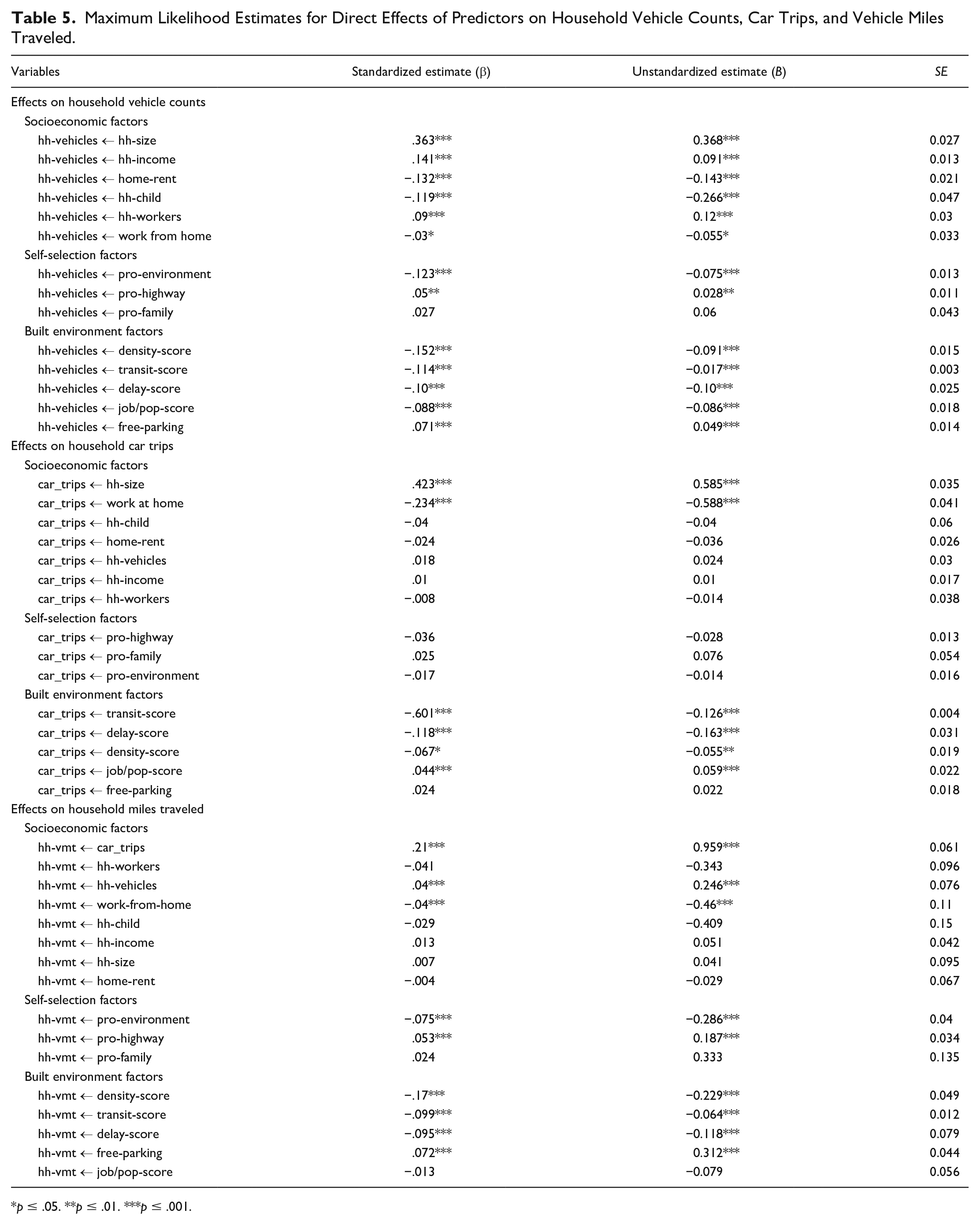
p ≤ .05. **p ≤ .01. ***p ≤ .001.

All household characteristics are significant predictors of household vehicle counts. The unstandardized coefficient for the effect of household size on household vehicle counts (B = 0.368) indicates that each additional person in the household is associated with a 36.8 percent increase in the number of vehicles in the household. This is consistent with our hypothesis. As expected, each additional worker in the household is associated with an increase in the number of household vehicles by 12 percent (B = 0.12). As hypothesized, household income is positively associated with the number of vehicles in the household. The B (=0.091) indicates that one-dollar increase in income corresponds to 9.1 percent increase in number of household vehicles. Compared with homeowner households, households living in rental homes own 14.3 percent fewer vehicles (B = −0.143). Also as expected, households with workers who have the option of working from home tend to own fewer vehicles than those with workers who commute to work (B = −0.055). However, the B for number of children (=−0.266) shows a significant negative relationship between the number of children and household vehicles, all else being equal. This finding is at odds with our hypothesis and suggests that the relationship between the number of children and vehicles in a household is not straightforward. Some studies have found that on one hand, more children in a household increase the need for cars to carry children around for various activities and hence more vehicles in a household (e.g., see Caulfield 2012; Zegras and Hannan 2012). Other studies found that household vehicle ownership is related to the age of children and the stage in life cycle of adults. Specifically, “families with small children have a higher probability of reducing the number of household vehicles” because they have fewer activities than children in older age groups (Liu et al. 2020; Yamamoto 2008). Families with older children, especially those in the driving age, may have higher number of vehicles because of more drivers. Financial stress such as child support and mortgage for mid-age adults represents drain on discretionary income that would otherwise be spent on vehicle after controlling for household income and household size (Liu et al. 2020). These circumstances may explain the negative relationship between number of children and household vehicle count.

For self-selection attributes, households with pro-environmental attitudes tend to own fewer vehicles as hypothesized (B = −0.075). Also as expected, the pro-highway factor (B = 0.028) is positively associated with household vehicle counts. Despite the expected positive relationship between the pro-family factor and vehicle counts (B = 0.06), this result does not reach statistical significance at the .05 level.

The results for the built environment variables are consistent with our hypotheses. The delay score, density score, job-population balance score, and transit score are inversely associated with the number of household vehicles. For instance, households living in congested areas tend to own fewer vehicles than households living in uncongested areas (B = −0.10). Each point rise in the delay score is associated with a 10 percent decrease in the quantity of household vehicles. Each point increase in the density score is associated with a 9.1 percent decline in number of household vehicles. This finding supports the hypothesis that people living in dense areas tend to have fewer cars. The same relationship is observed in the relationship between job-population balance and household vehicle counts (B = −0.086). Similarly, each point increase in the transit score is associated with a 1.7 percent decline in the number household vehicles (B = −0.017). On the other hand, households with access to free parking tend to own more vehicles than those that do not (B = 0.049).

The standardized estimates reveal that household characteristics have greater effects on household vehicle counts than the other two categories. In particular, household size is the most influential predictor (β = .363), and household income, homeownership, and number of children also play significant roles. The roles of built environment factors are also significant as shown by the β’s for density score, transit score, and delay score. The self-selection factors appear to be weakest. Especially, the pro-family attitude is the least influential determinant of vehicle count (β = .027). But the pro-environment factor cannot be ignored (β = −.123).

Number of Car Trips

The results in Table 5 indicate that among household characteristics, only household size and working from home status have significant direct effects on the number of household car trips. Specifically, each additional person in the household corresponds with a 58.5 percent increase in number of household car trips (B = 0.585). Working from home is associated with 58.8 percent reduction in number of household car trips (B = −0.588). Other household factors do not have statistically significant effects at the .05 level. Table 5 also shows that none of the self-selection factors attains statistical significance at the .05 level, indicating they have no significant effects on the number of household vehicle trips.

As hypothesized, most of the built environment variables are related to household vehicle trips significantly. Delay score and density factor show a negative association with the number of car trips. Each point increase in the delay score is associated with a 16.3 percent drop in the number of household car trips (B = −0.163). Each additional point in the density score is correlated with 5.5 percent decline in the household car trips (B = −0.055). Access to public transit, a built environment factor, also shows a reduction in the number of household car trips (B = −0.126) by 12.6 percent. Each point increase in the job/pop score is associated with a 5.9 percent increase in car trips (B = 0.059). Access to free parking makes no significant difference in the number of vehicle trips.

The standardized estimates indicate that transit score is the most significant contributor to reduction in car trips (β = −.601), followed by working at home and delay score (β = −.234 and β = −.118, respectively), among others. On the other hand, household size is the most influential factor that increases the number of household vehicle trips (β = .423).

VMT

Several patterns emerge from the results of the last panel in Table 5 predicting VMT, our ultimate outcome variable. First, both mediating variables (also considered part of the household characteristics)—number of household vehicle trips and number of household vehicles—are significant positive predictors of daily VMT. As expected, each vehicle trip is associated with an increase in VMT by 95.9 percent (B = 0.959), and the number of vehicle trips is the most important predictor of VMT among all predictors (β = .21). Also as anticipated, each additional household vehicle is correlated with an increase in VMT by about 25 percent (B = 0.246). Second, most other household characteristics do not show significant direct impact on VMT, except for working from home. Working from home does lower VMT by 46 percent compared with not working from home (B = −0.46). Third, self-selection factors appear to be by and large significant predictors of VMT. Households that indicated a higher level of importance for selecting their residential locations based on access to highways tend to have higher VMTs (B = 0.187). In contrast, the pro-environment factor is found to be a significant suppressor of daily household VMT (B = 0.286). The pro-family factor does not make a significant difference in VMT.

Finally, most built environment variables contribute significantly to VMT. As hypothesized, traffic delay reduces VMT (B = −0.118); that is, each point increase in delay score is associated with 11.8 percent reduction in VMT per household. Also as expected, each point increase in density score is associated with 22.9 percent reduction in VMT (B = −0.229). This is consistent with the findings of Ewing, Tian, and Lyons (2018) and Kim and Brownstone (2013). As hypothesized, households located in areas with closer proximity to transit tend to have a lower daily household VMT (B = −0.064). In contrast, households with access to free parking have a higher daily VMT by 31.2 percent (B = 0.312), compared to those without access to free parking. The job-population balance score does not have a significant effect on VMT. We also tested the interaction effect between the transit and delay scores, but the result reveals an insignificant interaction effect, suggesting that the effect of traffic delay does not vary significantly by transit availability.

The standardized estimates indicate that number of car trips, density score, transit score, and delay score are among the most important predictors of VMT in terms of direct effect. Free parking and pro-environment attitudes also play a role. In short, selected household characteristics, self-selection factors, and environmental factors contribute significantly to household VMT.

Total, Direct, and Indirect Effects

The foregoing discussion pertains only to the direct effects, but one of the advantages of SEM is to produce estimates for three types of effects: direct, indirect, and total effects. Direct effect refers to the influence of one variable on another unmediated by any other variables in a path model. Indirect effect refers to an effect mediated by at least one intervening variable (Bollen 1989). The sum of the direct and indirect effects is the total effect. The direct, indirect, and the total effects of predictor variables on VMT per household are summarized in Table 6. The indirect effects are generally small, except for household size (β = .105). Among all the factors, number of trips by car has the highest total effect on VMT (β = .21), followed by the density score (β = −.191). The total effect of delay score, a key variable and focus of this investigation, is −.124. Access to transit is also a significant factor for reduction in VMTs. Free parking, on the other hand, is associated with higher VMT. Besides car trips, the total effect of household size is also significant. The total effects of other household and self-selection factors on VMT, albeit somewhat smaller compared with the aforesaid factors, are also displayed in Table 6. Together, these findings suggest that controlling for household and self-selection factors and congestion factor along with many built environment factors such as land use, parking, and transit all play an important role in VMT.

Table 6.

Standardized Estimates of Direct, Indirect, and Total Effects on VMT per Household.

Variables	Direct effect	Indirect effect	Total effect
Socioeconomic factors
car_trips	0.21		0.21
hh-Size	0.007	0.105	0.112
home-rent	−0.04	−0.051	−0.091
hh-vehicles	0.04	0.004	0.044
hh-num-workers	−0.041	0.002	−0.039
hh-num-children	−0.029	−0.006	−0.035
hh-income	0.013	0.006	0.019
work from home status	−0.004	−0.011	−0.015
Self-selection factors
pro-environment	−0.075	−0.009	−0.084
pro-highway	0.053	0.005	0.058
pro-family	0.024	0.006	0.03
Built environment factors
density-score	−0.17	−0.021	−0.191
delay-score	−0.095	−0.029	−0.124
transit-score	−0.099	−0.021	−0.12
free-parking	0.072	0.008	0.08
job/pop-score	−0.013	−0.005	−0.018

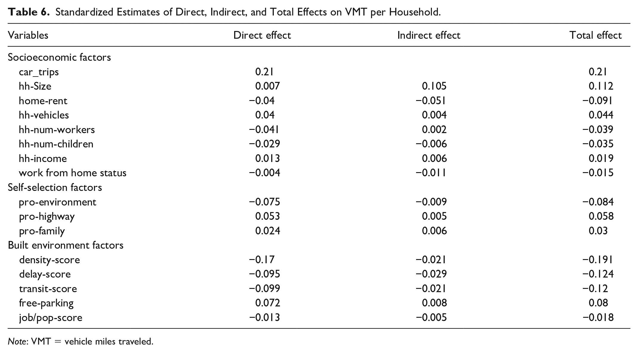
Note: VMT = vehicle miles traveled.

Conclusion

Scholars have debated about the effects of traffic congestion on greenhouse gas emissions, environmental justice, air pollution, public health, and physical activities, among others, yet few studies have directly considered its effect on travel behavior (Bovy and Salomon 2002; Litman 2014; Stern, Salomon, and Bovy 2002). This study fills this gap by investigating the impact of congestion, along with other built environment, self-selection, and socioeconomic factors, on VMT, both directly and indirectly based on data for the PSRC region/area. It contributes to the literature with an improved framework that incorporates household demographic and socioeconomic characteristics, self-selection factors, and built environment factors. Moreover, this study provides an improved measure of travel time delay that can differentiate traffic congestion from nonsaturated traffic condition with a normalized score. This delay score can also better reflect the local traffic condition without encumbering data collection and processing requirements. The delay score can be used to examine not only the effects of congestion on travel behavior measured by VMT but also the interrelationships among congestion, physical activities, obesity, or other public health outcomes. Finally, this research empirically tests a theory that was hypothesized several decades ago but has yet been tested. This research adds empirical evidence to the debate over planning policies with new data and SEM that can address measurement errors and complex relationships among observed and unobserved variables (Tomarken and Waller 2005).

Our research findings by and large are consistent with our research hypotheses about the effects of household characteristics, attitudes toward residential selection, and built environment conditions on travel behavior measured by VMT. All the variables included in this study, except for the pro-family factor, show direct influence on household vehicle counts. One unexpected result is the negative relationship between the number of children in a household and household vehicle counts, which might be explained by the age of children and/or stage in life cycle of adults in households. Household size, work at home, and all the environmental characteristics, except for free parking, are correlated with the number of car trips. All else being equal, household vehicle counts, household car trips, work from home, pro-highway, and pro-environment factors are significant predictors of VMT. Holding household characteristics and self-selection factors constant, the built environment variables play significant roles in VMT. The number of household vehicle trips, density score, traffic delay, and transit score are the four most influential factors in terms of total effect on VMT.

One important takeaway from this study is the influence of travel time delay on household vehicle counts, household vehicle trips, and VMT. The findings based on the PSRC data suggest that congestion has two sides. On one hand, congestion is annoying because it causes more time to travel, reduces productivity, increases vehicle emission and stress, and is also harmful to air quality and health. On the other hand, the results of this study reveal that travel delay, a measure of congestion, is associated with fewer household vehicles, fewer vehicle trips, and lower VMT. These are beneficial to environment and energy conservation. Congestion might also be seen as an adversary of density because congestion is more likely, though not always, to exist in areas with high density, a key paradox at the center of the land use policy debate. However, congestion can coexist with density as demonstrated by Mondschein and Taylor (2017). While “delay” is treated as a built environment variable in this study, it is a measure of the “mobile” feature of the built environment. This measure differs from other land use density and diversity variables that quantify the “fixed,” long-term features of the built environment. The findings about the effects of travel delay reinforce the notion that travel delay is an important constraint of travel behavior and should be considered along with other “D” factors. Together, they point to the need for comprehensive solutions, such as transportation demand management (TDM) policies² in addition to land use policies for managing travel demand. As argued by many scholars, congestion is more efficiently managed by congestion pricing policies, such as pricing by time, location, distance, vehicle occupancy, or other hybrid strategies depending on the nature of the challenges faced by communities. While “complete” pricing of transportation is difficult, other forms of congestion pricing are possible. For example, toll roads, value pricing strategies, high-occupancy toll (HOT)/managed lanes in California, Texas, and many areas have proven to be acceptable by the public. A common characteristic of these forms of congestion pricing is that the “priced” transportation services are offered as alternatives or choices to the “free” transportation infrastructure services. By providing “options,” travelers can make their decisions based on their preferences and other circumstances.

The findings about the effects of free parking offer support for parking management, also a TDM strategy. Shoup (2005a, 2005b) has long discussed the problems of free parking and proposed parking cash-out, along with charging the full price of parking as a win-win solution for employers, commuters, and the society as a whole. As explained by Shoup, parking cash-out is an excellent recruiting tool. Employers with parking cash-out can attract quality employees, retain current employees, and promote productivity as happy employees tend to perform better. Employees benefit from parking cash-out as they have the freedom to decide the best use of the cash and to make mode choice decisions. As commuters shift from driving to other modes of travel, society is better off with reduced traffic congestion, improved air quality, higher demand for transit, and more equity in transportation and public health.

The findings regarding densities and transit accessibility lend support to such land use policies as compact development, and mixed-use or TODs that combine residences, employment, and related services in pedestrian-friendly environments. Nonetheless, dense, mixed-use, or TODs in most large cities tend to be expensive and associated with less reputable public schools. To provide affordable housing with good schools, it is desirable to explore innovative policies such as subsidies, tax abatement, charter school, school choice, or other institutional collaborative approaches that can help control housing prices, improve educational quality and choice, and create a safe environment for urban and suburban residents to make residential location decisions. Through the adoption of land use, congestion pricing, and equity-based resource allocation policies with a holistic approach, it may be possible to create an “optimal equilibrium” in traffic congestion, land use density, and equity, though an “optimal equilibrium” accepted by the public in one region may be different from that in another region due to variations in social, political, and geographical contexts.

This research points to a number of directions for future planning research. First and foremost, since this study is based on the 2015 disaggregated NHTS data in one metropolitan area, the validity of the findings ought to be verified by additional empirical studies using the post-2015 data. Second, because of regional variations in social, political, and geographical contexts, future studies may further explore this issue using data for other regions. Third, future studies may investigate the effects of additional factors on travel behavior with panel data or other longitudinal travel data. Some examples of such additional factors are travel time reliability and moderating variables. Finally, future research may use different measures of certain variables included in this study. For example, density score in this study is a composite variable created with PCA. While this measure is useful, further research may consider separating the built environment density components into different types of densities to investigate their effects on travel behavior. It will also be useful to include commuters’ route choices in travel surveys, as this will allow one to analyze the effects of traffic congestion on another dimension of travel behavior. Doing some or all of these will further enhance our understanding of the effects of traffic congestion on travel behavior.

Footnotes

Acknowledgements

The authors wish to thank the three anonymous reviewers and the journal editors for their critical and constructive comments on an earlier version of the paper. They are grateful for the research facilities and support from the University of Texas, Arlington.

Declaration of Conflicting Interests

The author(s) declared no potential conflicts of interest with respect to the research, authorship, and/or publication of this article.

Funding

The author(s) received no financial support for the research, authorship, and/or publication of this article.

ORCID iD

Jianling Li

Notes

Author Biographies

Reza Sardari is a business intelligence analyst at the City of Plano, Texas. His research interests and expertise include integrated land use and transportation models, market share analysis, predictive models, and geospatial data analytics.

Jianling Li is a Professor of Urban Planning in the College of Architecture, Planning and Public Affairs, at the University of Texas, Arlington. Her areas of research interests include transportation policies, travel behavior, data analytics, smart cities, and public health.

Raha Pouladi is a lead planner at the City of Plano, Texas. Her research interests are urban planning, placemaking, affordable housing, urban beautification, and gentrification.

References

Badland

H. M.

Oliver

Kearns

R. A.

Mavoa

Witten

Duncan

M. J.

Batty

G. D.

2012. “Association of Neighbourhood Residence and Preferences with the Built Environment, Work-Related Travel Behaviours, and Health Implications for Employed Adults: Findings from the URBAN Study.” Social Science and Medicine 75 (8): 1469–76. doi:10.1016/j.socscimed.2012.05.029.

Bagley

M. N.

Mokhtarian

P. L.

2002. “The Impact of Residential Neighborhood Type on Travel Behavior: A Structural Equations Modeling Approach.” The Annals of Regional Science 36 (2): 279–97. doi:10.1007/s001680200083.

Beaver

S. H.

1956. “Review of Urban Traffic: A Function of Land Use.” [Review of Review of Urban Traffic: A Function of Land Use, by Robert B. Mitchell and C. Rapkin]. Population Studies 10 (1): 117–17. doi:10.2307/2172279.

Ben-Akiva

Lerman

S. R.

1985. Discrete Choice Analysis: Theory and Application to Travel Demand. Vol. 9. Cambridge: MIT Press.

Bohte

Maat

van Wee

2007. “Residential Self-Selection. The Effect of Travel-Related Attitudes and Lifestyle Orientation on Residential Location Choice; Evidence from the Netherlands.” 11th World Conference on Transport Research, Berkeley, CA, June 24–28. https://trid.trb.org/view/884684.

Bollen

K. A.

1989. Structural Equations with Latent Variables. Hoboken: Wiley.

Bovy

P. H.

Salomon

2002. “Congestion in Europe: Measurements, Patterns and Policies.” In Travel Behaviour: Spatial Patterns, Congestion and Modelling, edited by Stern

Salomon

Bovy

P. H. L.

, 143–179. Cheltenham: Edward Elgar Publishing.

Byrne

B. M.

2012. Structural Equation Modeling with Mplus: Basic Concepts, Applications, and Programming. New York: Routledge/Taylor & Francis Group.

Cao

Chatman

2015. “How Will Smart Growth Land-Use Policies Affect Travel? A Theoretical Discussion on the Importance of Residential Sorting.” Environment and Planning B: Planning and Design 43: 58–73. doi:10.1177/0265813515600060.

10.

Cao

Mokhtarian

Handy

2009. “Examining the Impacts of Residential Self-Selection on Travel Behaviour: A Focus on Empirical Findings.” Transport Reviews 29 (3): 359–95.

11.

Caulfield

2012. “An Examination of The Factors That Impact Upon Multiple Vehicle Ownership: The Case of Dublin, Ireland,” Transport Policy, 19 (1): 132–138. doi:10.1016/j.tranpol.2011.08.003

12.

Cervero

1989. “Jobs-Housing Balancing and Regional Mobility.” Journal of the American Planning Association 55 (2): 136–50. doi:10.1080/01944368908976014.

13.

Cervero

1996. “Mixed Land-Uses and Commuting: Evidence from the American Housing Survey.” Transportation Research Part A: Policy and Practice 30 (5): 361–77. doi:10.1016/0965-8564(95)00033-X.

14.

Cervero

Kockelman

1997. “Travel Demand and the 3Ds: Density, Diversity, and Design.” Transportation Research Part D: Transport and Environment 2 (3): 199–219. doi:10.1016/S1361-9209(97)00009-6.

15.

Christiansen

Engebretsen

Ø.

Fearnley

Usterud Hanssen

2017. “Parking Facilities and the Built Environment: Impacts on Travel Behaviour.” Transportation Research Part A: Policy and Practice 95:198–206. doi:10.1016/j.tra.2016.10.025.

16.

Crane

Chatman

D. G.

2003. Traffic and Sprawl: Evidence from US Commuting from 1985-1997. Vol. 6. Los Angeles: University of Southern California.

17.

De Vos

Derudder

Van Acker

Witlox

2012. “Reducing Car Use: Changing Attitudes or Relocating? The Influence of Residential Dissonance on Travel Behavior.” Journal of Transport Geography 22:1–9. doi:10.1016/j.jtrangeo.2011.11.005.

18.

Downs

1992. Stuck in Traffic. Washington, DC: Brookings Institution Press.

19.

Downs

2004. Still Stuck in Traffic: Coping with Peak-hour Traffic Congestion. Washington, DC: Brookings Institution Press.

20.

Ewing

1994. “Residential Street Design: Do the British and Australians Know Something Americans Do Not?” Transportation Research Record 1455. https://trid.trb.org/view/424730.

21.

Ewing

1997. “Is Los Angeles-Style Sprawl Desirable?” Journal of the American Planning Association 63 (1): 107–26.

22.

Ewing

Bartholomew

2018. Best Practices in Metropolitan Transportation Planning. New York: Routledge.

23.

Ewing

Cervero

2001. “Travel and the Built Environment: A Synthesis.” Transportation Research Record: Journal of the Transportation Research Board 1780:87–114. doi:10.3141/1780-10.

24.

Ewing

Cervero

2010. “Travel and the Built Environment: A Meta-Analysis.” Journal of the American Planning Association 76 (3): 265–94. doi:10.1080/01944361003766766.

25.

Ewing

Deanna

S.-C.

1996. “Land Use Impacts on Trip Generation Rates.” Transportation Research Record: Journal of the Transportation Research Board 1518:1–6. doi:10.3141/1518-01.

26.

Ewing

Pendall

Chen

2003. “Measuring Sprawl and Its Transportation Impacts.” Transportation Research Record: Journal of the Transportation Research Board 1831:175–83. doi:10.3141/1831-20.

27.

Ewing

Tian

Lyons

2018. “Does Compact Development Increase or Reduce Traffic Congestion?” Cities 72:94–101. doi:10.1016/j.cities.2017.08.010.

28.

Federal Highway Administration. 2017. “Explore Vehicle Trips Data: Popular Vehicle Trips Statistics—Trip Purpose.” https://nhts.ornl.gov/vehicle-trips.

29.

Federal Highway Administration. 2022. “Transportation Demand Management.” https://ops.fhwa.dot.gov/plan4ops/trans_demand.htm.

30.

Foster

Jeremy J.

Barkus

Yavorsky

2006. Understanding and Using Advanced Statistics. London: SAGE.

31.

Frank

L. D.

Saelens

B. E.

Powell

K. E.

Chapman

J. E

. 2007. “Stepping towards Causation: Do Built Environments or Neighborhood and Travel Preferences Explain Physical Activity, Driving, and Obesity?” Social Science and Medicine 65 (9): 1898–1914. doi:10.1016/j.socscimed.2007.05.053.

32.

Gillham

2002. The Limitless City: A Primer on the Urban Sprawl Debate. Washington, DC: Island Press.

33.

Google LLC. 2018. “Google Maps Platform Terms of Service.” https://cloud.google.com/maps-platform/terms/.

34.

Gordon

Lee

. 2015. “Spatial Structure and Travel: Trends in Commuting and Non-commuting Travels in US Metropolitan Areas.” In Handbook on Transport and Development, edited by Hickman

Bonilla

Givoni

Banister

, 87–103. Cheltenham: Edward Elgar Publishing. https://www.elgaronline.com/view/edcoll/9780857937254/9780857937254.00012.xml.

35.

Gordon

Richardson

H. W.

1997. “Are Compact Cities a Desirable Planning Goal?” Journal of the American Planning Association 63 (1): 95–106. doi:10.1080/01944369708975727.

36.

Gordon

Richardson

H. W.

Jun

M. J.

1991. “The Commuting Paradox: Evidence from the Top Twenty” Journal of American Planning Association 57 (4): 416–20. doi:10.1080/01944369108975516.

37.

Grace

J. B.

Johnson

D. J.

Lefcheck

J. S.

Byrnes

J. E.

2018. “Quantifying Relative Importance: Computing Standardized Effects in Models with Binary Outcomes.” Ecosphere 9(6): e02283. doi:10.1002/ecs2.2283.

38.

Guerra

Caudillo

Goytia

Quiros

T. P.

Rodriguez

2018. “Residential Location, Urban Form, and Household Transportation Spending in Greater Buenos Aires.” Journal of Transport Geography 72:76–85. https://trid.trb.org/view/1540595.

39.

Holcombe

R. G.

Williams

D. W.

2010. “Urban Sprawl and Transportation Externalities.” Review of Regional Studies 40 (3): 257–73.

40.

Hox

J. J.

Bechger

T. M.

2007. “An Introduction to Structural Equation Modeling.” Family Science Review 11:354–73.

41.

Kamruzzaman

Baker

Washington

Turrell

2013. “Residential Dissonance and Mode Choice.” Journal of Transport Geography 33:12–28. doi:10.1016/j.jtrangeo.2013.09.004.

42.

Kim

Brownstone

2013. “The Impact of Residential Density On Vehicle Usage And Fuel Consumption: Evidence From National Samples.” Energy Economics 40: 196–206.

43.

Lamíquiz

P. J.

López-Domínguez

2015. “Effects of Built Environment on Walking at the Neighbourhood Scale. A New Role for Street Networks by Modelling their Configurational Accessibility?” Transportation Research Part A: Policy and Practice 74:148–63. doi:10.1016/j.tra.2015.02.003.

44.

Levinson

D. M.

Kumar

1997. “Density and the Journey to Work.” Growth and Change 28 (2): 147–72. doi:10.1111/j.1468-2257.1997.tb00768.x.

45.

2018. “Residential and Transit Decisions: Insights from Focus Groups of Neighborhoods around Transit Stations.” Transport Policy 63:1–9. doi:10.1016/j.tranpol.2017.10.012.

46.

Litman

2014. “Congestion Evaluation Best Practices.” International Transportation Economic Development Conference. I-TED 2014, Dallas, TX. https://pdfs.semanticscholar.org/8cb4/de716d755b9ed793c60a1bc2b414bf3b0d02.pdf.

47.

Liu

Nambisan

2020. “Are Young Americans Carless Across the United States? A Spatial Analysis.” Transportation Research Part D 78: 102197.

48.

Majid

M. R.

Nordin

A. N.

Medugu

I. N.

2014. “Influence of Housing Development Designs on Household Vehicle Miles Traveled: A Case of Iskandar Malaysia.” Transportation Research Part D: Transport and Environment 33:63–73. doi:10.1016/j.trd.2014.09.001.

49.

Mitchell

R. B.

Rapkin

1954. Urban Traffic: A Function of Land Use. New York: Columbia University Press.

50.

Mondschein

Taylor

B. D.

2017. “Is Traffic Congestion Overrated? Examining the Highly Variable Effects of Congestion on Travel and Accessibility.” Journal of Transport Geography 64:65–76. doi:10.1016/j.jtrangeo.2017.08.007.

51.

Næss

Strand

Wolday

Stefansdottir

2019. “Residential Location, Commuting and Non-Work Travel in Two Urban Areas of Different Size and with Different Center Structures.” Progress in Planning 128:1–36.

52.

Olaru

Smith

Taplin

J. H

. 2011. “Residential Location and Transit-Oriented Development in a New Rail Corridor.” Transportation Research Part A: Policy and Practice 45 (3): 219–37.

53.

Puget Sound Regional Council. 2015. “2015 Travel Surveys Program: Appendix 1—Questionnaire.” https://www.psrc.org/our-work/household-travel-survey-program.

54.

Salon

2009. “Neighborhoods, Cars, and Commuting in New York City: A Discrete Choice Approach.” Transportation Research Part A: Policy and Practice 43 (2): 180–96. doi:10.1016/j.tra.2008.10.002.

55.

Sangkapichai

Saphores

J. D

. 2009. “Why are Californians interested in hybrid cars?” Journal of Environmental Planning and Management 52 (1): 79–96. doi:10.1080/09640560802504670.

56.

Sardari

Hamidi

Pouladi

2018. “Effects of Traffic Congestion on Vehicle Miles Traveled.” Transportation Research Record 2672:92–102. doi:10.1177/0361198118791865.

57.

Sarzynski

Wolman

H. L.

Galster

Hanson

2006. “Testing the Conventional Wisdom about Land Use and Traffic Congestion: The More We Sprawl, the Less We Move?” Urban Studies 43 (3): 601–26. doi:10.1080/00420980500452441.

58.

Schrank

D. L.

Albert

Luke

Eisele

Bill

Lomax

Tim J.

2021. The 2019 Urban Mobility Report. College Station, TX: Texas A&M Transportation Institute. https://static.tti.tamu.edu/tti.tamu.edu/documents/mobility-report-2021.pdf.

59.

Shoup

2005a. Parking Cash Out. Chicago, IL: American Planning Association.

60.

Shoup

2005b. The High Cost of Free Parking. Chicago, IL: American Planning Association.

61.

Stern

Salomon

Bovy

P. H.

, eds. 2002. Travel Behaviour: Spatial Patterns, Congestion and Modelling. Cheltenham: Edward Elgar Publishing.

62.

Stevens

M. R.

2017. “Does Compact Development Make People Drive Less?” Journal of the American Planning Association 83 (1): 7–18.

63.

Tomarken

A. J.

Waller

N. G.

2005. “Structural Equation Modeling: Strengths, Limitations, and Misconceptions.” Annual Review of Clinical Psychology 1 (1): 31–65.

64.

Van Acker

Mokhtarian

P. L.

Witlox

2011. “Going Soft: On How Subjective Variables Explain Modal Choices for Leisure Travel.” European Journal of Transport and Infrastructure Research 11 (2). doi:10.18757/ejtir.2011.11.2.2919.

65.

Van Wee

. 2009. “Self-Selection: A Key to a Better Understanding of Location Choices, Travel Behaviour and Transport Externalities?” Transport Reviews 29 (3): 279–92. doi:10.1080/01441640902752961.

66.

Wallace

D. A.

1956. “Review of Urban Traffic, A Function of Land Use” [Review of Review of Urban Traffic, A Function of Land Use, by R. B. Mitchell and C. Rapkin]. Journal of the American Statistical Association 51 (274): 417–18. doi:10.2307/2281388.

67.

Wang

2012. Structural Equation Modeling: Applications Using Mplus. Hoboken: Wiley, Higher Education Press. doi:10.1002/9781118356258.

68.

Yamamoto

2008. “The Impact of Life-Course Events On Vehicle Ownership Dynamics: The Cases of France and Japan.” IATSS Research 32 (2): 34–43.

69.

Zahabi

S. A. H.

Miranda-Moreno

Patterson

Barla

2015. “Spatio-Temporal Analysis of Car Distance, Greenhouse Gases and The Effect of Built Environment: A Latent Class Regression Analysis.” Transportation Research Part A: Policy and Practice 77:1–13. doi:10.1016/j.tra.2015.04.002.

70.

Zegras

P. C.

Hannan

V. A.

2012. “Dynamics of Automobile Ownership under Rapid Growth: Case Study of Santiago, Chile.” Transportation Research Record 2323 (1): 80–89. doi:10.3141/2323-10.

Delay: The Next “D” Factor in Travel Behavior?

Abstract

Keywords

Introduction

Urban Structure, Travel Behavior, and Traffic Congestion

The Effects of the “D” Factors

The Influence of Self-Selected Factors

Traffic Congestion on Travel Behavior: A Reversed Impact?

Method

Conceptual Model and Research Hypotheses

Data, Variables, and Measurements

Results

Model Fit Statistics

Household Vehicle Counts

Number of Car Trips

VMT

Total, Direct, and Indirect Effects

Conclusion

Footnotes

Acknowledgements

Declaration of Conflicting Interests

Funding

ORCID iD

Notes

Author Biographies

References