
Abstract
This article explores differences in the relationship between the built environment and households’ car use in Mexico City in 1994 and 2007. After controlling for income and other household attributes, population and job density, transit and highway proximity, destination diversity, intersection density, and accessibility are statistically correlated with households’ weekday car travel in Mexico City. These correlations are generally stronger than those found in studies from U.S. cities and fairly stable over time. Where correlations have changed, they have strengthened. Findings suggest that land use planning can play a modest and growing role in reducing car travel in Mexico City.
Introduction
Developing-world cities account for the lion’s share of recent and projected global population growth. A rapid increase in urban footprints—as cities sprawl outward—and car ownership and vehicle travel have accompanied this growth (Angel et al. 2011; Schafer and Victor 2000; Sperling and Clausen 2002; Sperling and Gordon 2009). Mexico City is no exception. Although aggregate metropolitan population growth has slowed markedly in the past two decades, the periphery continues to grow rapidly and accounts for nearly all recent and projected population growth. From 1990 to 2010, the metropolitan car fleet more than doubled. Between 1994 and 2007, total vehicle kilometers of car travel (VKT) on an average weekday increased from 24 million to 32 million. 1 Given the associated congestion, pollution, infrastructure, and public health costs, citizens, policy makers, and advocacy groups are increasingly interested in containing and slowing the rapid rise in automobility. Land use planning offers one opportunity.
Researchers have long found that people are less likely to drive and more likely to take transit, walk, or bike in dense built environments with a diverse mix of land uses. In Mexico, several prominent civil society organizations are encouraging the central government’s National Development Plan (2013–2018) to focus on increasing urban densities, decreasing peripheral growth, and concentrating development in metropolitan centers (Tapia 2013). However, most of our understanding of how the built environment influences individuals’ travel decisions comes from cross-sectional studies in American or European cities. What role can land use planning play in constraining car use in developing-world cities that are already dense and diverse? Is the built environment becoming more or less important as cities expand and more households move into peripheral neighborhoods? That is, does land use planning in Mexico City have increasing or diminishing returns over time?
To address these questions, this study analyzes and compares the empirical relationships between eight measures of the built environment and average weekday VKT in Mexico City in 1994 and 2007. The proceeding sections describe existing findings about the relationship between travel and the built environment; present hypotheses about the nature of this relationship in Mexico City relative to other cities and over time; document recent changes in the built environment and travel in Mexico City; describe the study’s data and statistical methods; present the results of the statistical models; and discuss the implications of the results for our understanding of the relationship between the built environment and travel and public policy in Mexico City.
The Built Environment and Travel Behavior across Places and over Time
After a long and lively debate, something of a general consensus about the influence of the built environment on car use has emerged in the United States: Small increases in density, land use diversity, and other quantifiable aspects of the built environment tend to contribute to statistically significant, but smaller decreases in households’ propensity to own and use cars (Bento et al. 2005; Boarnet 2011; Brownstone 2008; Ewing and Cervero 2010; Transportation Research Board 2009; Frank et al. 2008; Zhang 2006). Regional metrics, such as distance from the downtown or job accessibility, have a stronger but still less than proportional effect. Despite many similarities in empirical findings, there is no reason to expect the influence of the built environment on car travel to be stable either across geographies or over time; particularly in rapidly growing developing-world cities where densities are much higher, public transportation is more readily available, and households are generally larger and poorer.
Empirical Findings from Developing-World Cities
Empirical studies from developing-world cities also generally find statistically significant correlations between quantifiable aspects of the built environment, car ownership and use (Cao, Chen, and Zhen 2009; Shirgaokar 2012; Zegras 2010; Zegras and Hannan 2012; Zhang 2004), and nonmotorized travel (Cervero et al. 2009; Sallis et al. 2009). However, the relationships are not systematically stronger than those observed in the United States. For example, Zegras’s (2010) estimates of the collective strength of the relationship between the built environment variables and car travel in Santiago de Chile is around twice the average from Ewing and Cervero’s (2010) meta-analysis, which primarily consists of U.S.-based studies. By contrast, Zhang (2004) finds a stronger correlation between local population density and travel behavior in Boston than in Hong Kong. Job density has a similar relationship in both cities. Hong Kong, however, is so dense—average households lived in neighborhoods with 650 residents per hectare (263 per acre)—that a weaker statistical correlation at the margin is unsurprising. The built environment and other factors already constrain most car trips. Only 8.6 percent of work trips and 6.6 percent of nonwork trips in the sample rely on cars.
Research Hypotheses
Two hypotheses about the general nature of the relationship between the built environment and car use in Mexico City guide this research. For a review of the hypothesized relationships between individual measures of the built environment and car use and empirical findings from more than two hundred studies, I refer readers to Ewing and Cervero (2010).
Hypothesis 1: The relationship between the built environment and car use in Mexico City tends to be stronger than the relationship observed in U.S. cities.
In theory, the built environment influences household car use through its influence on the relative cost and availability of different travel alternatives for achieving day-to-day activities like work, shopping, and recreation (Boarnet and Crane 2001; Chatman 2008; Crane 2000; Handy 1996a, 1996b). Facing shorter trip distances, more congestion, higher car-insurance fees, less parking, higher gasoline prices, better public transit, and a more pleasant walking environment, residents tend to drive less in dense, compact cities than in sparse, sprawling ones. Above or below a certain threshold, however, changes in the built environment are likely to have little or no effect on travel because they no longer influence the relative attractiveness of travel choices. For example, Pickrell (1999) observed no correlation between household car use and residential population density below 15 people per gross hectare (6 per acre) in the United States. The relationship only became pronounced above 29 people per gross hectare (12 per acre). Newman and Kenworthy (2006) identified a similar threshold of 35 jobs and people per gross hectare (14 per acre) across fifty-eight high-income cities around the world. In Mexico City, like most other developing-world metropolises, density levels are significantly higher than this minimum. Even the most peripheral neighborhoods had an average of 54 people per hectare in 2005. On the one hand, nearly all of Mexico City’s residents live in neighborhoods that are sufficiently dense to influence travel choices. On the other, if all neighborhoods are extremely dense, density may not covary much with households’ travel within a city, as Cervero et al. (2009) found in a study of land use and nonmotorized travel in Bogota.
The influence of the built environment also depends on the relative desirability of travel options, independent of the built environment. For example, if a traveler is indifferent between driving a car and taking the bus for a given trip, any small change in the cost or convenience of either mode will likely influence mode choice. By contrast, even significant changes to the cost or convenience of the bus will be unlikely to influence the traveler’s mode choice, if the time-savings and convenience of driving significantly outweigh the bus’s lower costs. Barring some radical nonlinear differences in a population—for example, everyone above median income drives, while everyone below takes the bus—changes to the built environment are likely to have the strongest influence on aggregate mode choice where roughly the same proportion of individuals chooses each option. Given that Mexico City’s residents used cars for one-third of nonpedestrian trips on an average weekday (INEGI 2007a), the relative attractiveness of alternatives to the car—whether due to lower incomes, greater congestion, or better public transportation—is presumably much higher than in the United States, where nearly all trips are made by car (U.S. Department of Transportation 2009) or Hong Kong, where very few are.
Hypothesis 2: The relationship between the built environment and car use in Mexico City has changed over time.
In addition to differences across cities, the relationship between different aspects of the built environment and travel behavior is unlikely to remain stable in the rapidly changing cities of the developing world. On the one hand, more residents tend to live in less dense neighborhoods of the periphery, as the metropolis expands. On the other hand, rising incomes and car use may strengthen the constraining influence of the built environment, since more people are competing for scarce road space and parking. Few empirical studies, however, examine more than a single cross-sectional snapshot of individual travel behavior. In a rare exception, Zegras and Hannan (2012) model car ownership in Santiago de Chile in 1991 and 2001. They find notable changes in household behavior over the period and estimate that the influence of neighborhood population density on car ownership doubled over the time period while the influence of land use diversity decreased significantly. Proximity to the subway went from having a statistically insignificant correlation with car ownership in 1991 to a significant one in 2001. While the modeling structure does not allow for direct comparison of the parameter estimates—they reject the hypothesis that preferences have remained stable but do not normalize parameter estimates across the two time periods—it is nevertheless clear that the estimated influence of the built environment on car ownership changed in a significant and measurable way in just ten years. This study builds on directly on this previous work by adding another empirical example of how the relationship between the built environment and household travel behavior has changed over time in a fast-changing, developing-world city. It also expands research in this area by focusing on car use, rather than car ownership, and by providing directly comparable parameter estimates and statistical tests of whether and how the relationship has changed.
Case Context, Data, and Model Specifications
Case Context
The Mexico City Metropolitan Area’s population has grown at an average annual rate of 10 percent since 1950. Although aggregate growth rates have slowed considerably in recent years, many suburban neighborhoods grew at more than 10 percent annually between 1990 and 2010. During that period, the proportion of metropolitan residents living outside of the Federal District—the jurisdictional limits of Mexico City proper—increased from 44 to 53 percent. Car ownership and use also increased. Table 1 summarizes recent demographic and travel trends in Mexico City between 1994 and 2007. A suburbanizing metropolis and increased driving in the suburbs account for nearly all of the 33 percent increase in total weekday VKT from 24 million to 32 million. Average one-way travel time increased from an already high 47 minutes to 51 minutes across the metropolis.
Population and Travel in Mexico City between 1994 and 2007.
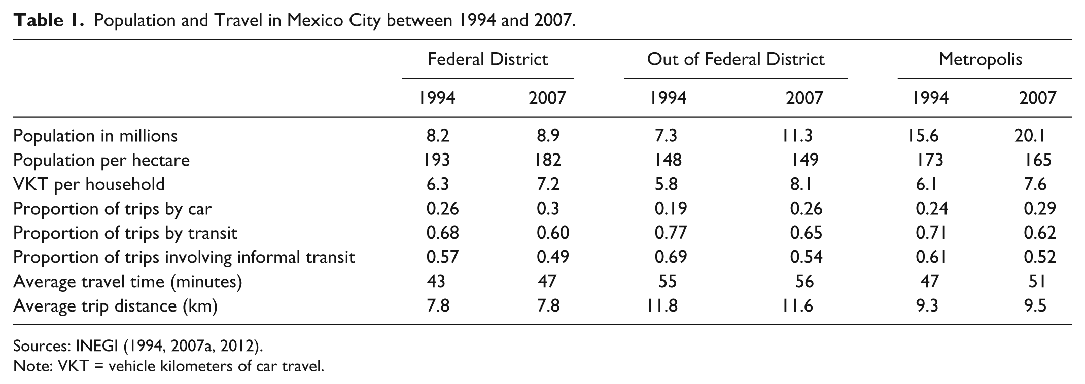
Sources: INEGI (1994, 2007a, 2012).
Note: VKT = vehicle kilometers of car travel.
Nevertheless, peripheral households remained less likely to drive than more centralized households in 2007. Figure 1 maps the percentage of households that generated any VKT on the weekday of the 2007 travel survey by municipality and borough. This correlates well with a map of household income; households in the wealthier western parts of the city are more likely to drive. Once a household generates VKT, however, geographic centrality has a clear spatial correlation with how much they drive (Figure 2).
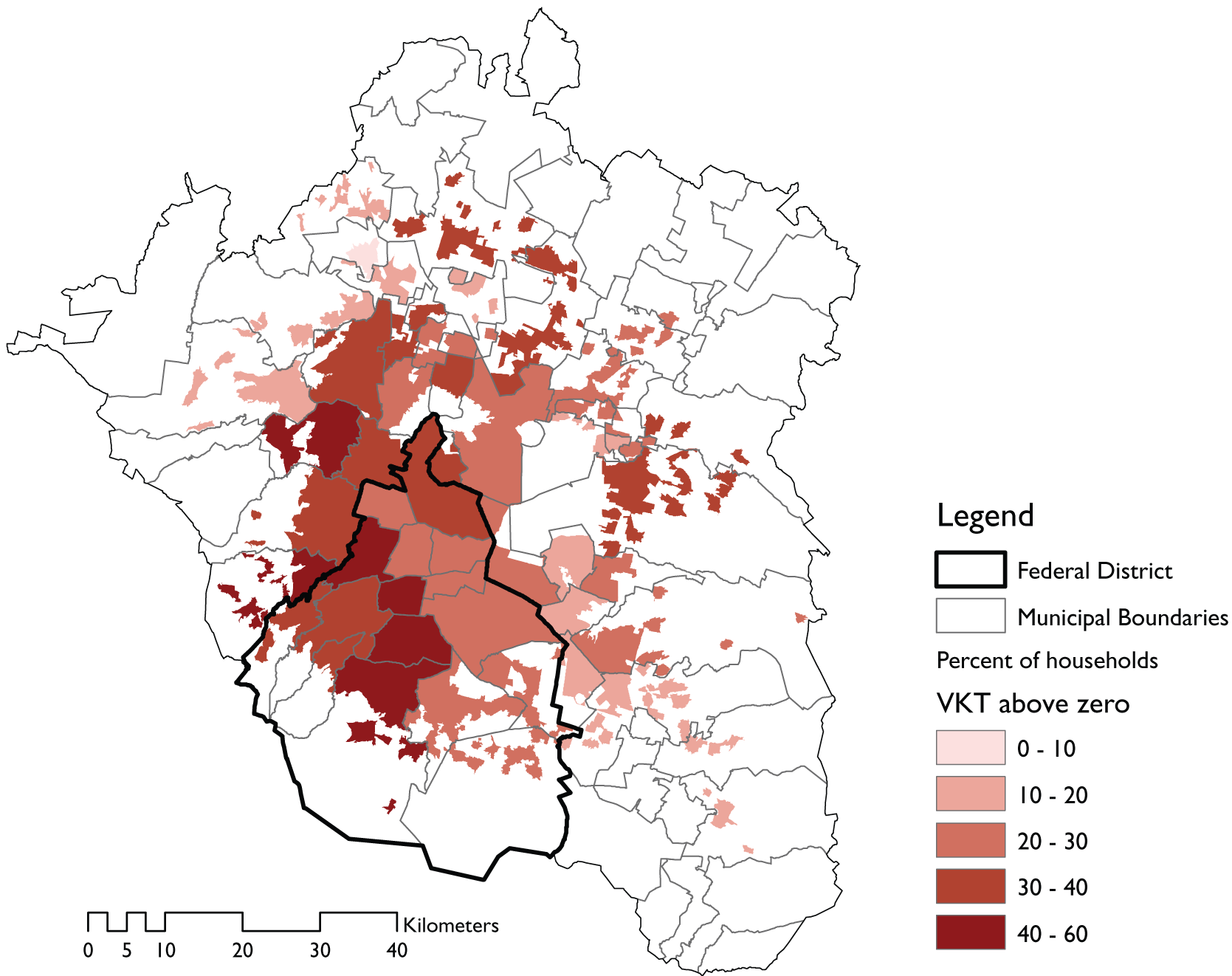
Percentage of households that generated vehicle kilometers of car travel (VKT) on survey day in 2007.
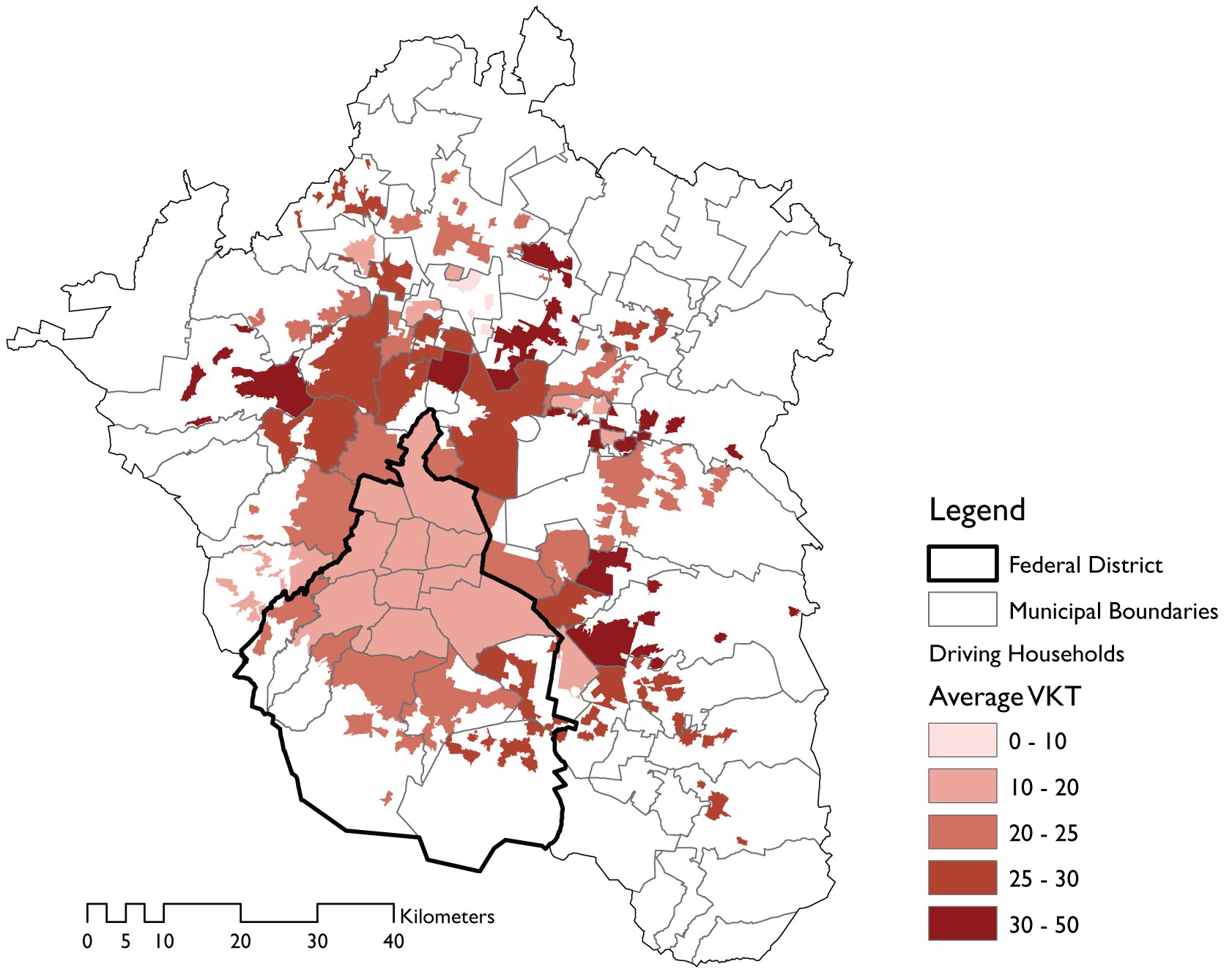
Average daily vehicle kilometers of car travel (VKT) per driving household on survey day in 2007.
Despite a suburbanizing metropolis, Mexico City’s jobs have remained fairly centralized. The four oldest and most central boroughs accounted for half of metropolitan Gross Census Value Added, a measure of economic output, and 34 percent of formal metropolitan jobs in 2008 (INEGI 2012). The central boroughs had 123 jobs per hectare compared to 5 per hectare in the most remote municipalities in 2008. Furthermore, Mexico City has a fairly flat population distribution. In 2005, two-thirds of all metropolitan residents lived in neighborhoods with densities between 100 and 300 people per hectare (40 and 120 per acre). Many of the densest of these neighborhoods are in large inner suburbs like Ecatepec and Nezahualcoyotl, which together house nearly three million residents. This density combined with widespread informal public transit and a centralized high-capacity metro system has allowed Mexico City to maintain high transit mode share in suburban as well as central locations (Table 1). In 2007, despite a decline in mode share from 1994, a majority of all metropolitan trips relied on informal transit in privately owned minivans or minibuses for at least one trip segment.
Between 1994 and 2007, the metro added 24 kilometers of new right-of-way to the 178-kilometer system, significantly increasing service into the southeast and northeast. While ridership on these two new lines has been high, aggregate metro ridership has remained flat (Guerra 2014). Despite the increased metro service, a smaller fraction of metropolitan households lived near the metro in 2007 than in 1994 because of decreasing population densities around stations in the Federal District and population growth in peripheral neighborhoods far from the metro (Guerra 2014).
Data
The National Statistics and Geography Agency (INEGI 1994, 2007a) conducted metropolitan household travel surveys in 1994 and 2007. The surveys contain information on approximately 1 percent of all households, household members, and their daily travel—including the geographic location of origins and destinations, trip purpose, trip duration, trip time, out-of-pocket expenses, and mode of travel—on an average weekday in the Mexico City Metropolitan Area (Zona Metropolitana del Valle de México). 2 The surveys exclude pedestrian travel and travel by children younger than six. Both surveys provide geographic codes for household location, origin, and destination to the Census Tract (Área Geográfico Estadística Básica) and sample weights based on full Census data for each household and trip. 3 I spatially matched the surveys with 1990 and 2005 Census shapefiles, a national municipal database (INEGI 2012), and transportation infrastructure from the National Statistics and Geography Agency (INEGI 2013), the Secretary of Transportation and Highways (SETRAVI 2013), and OpenStreetMap (2013) to estimate local population and job densities, accessibility measures, and distance from metro stations, major highways, and the center of the city. Data cleaning led to the exclusion of 2,433 households from the 1994 data set and 5,324 from 2007, generally because of unreported income (1,974 missing from 1994 and 4,708 missing from 2007) but also because of unmatched or mislabeled home Census Tracts (484 missing from 1994 and 639 from 2007).
Table 2 provides data means and standard deviations for all variables used in this study. Because of a limitation in the 1994 database, household-level statistics are approximated from the available information on individuals who took trips during the survey day in 1994 and 2007. In 2007, approximately half of all household members reported taking a trip (an average of 2.23 compared to an average household size of 4.07). Children between 6 and 10 were less likely to travel; only about a seventh of those surveyed reported having taken vehicular trips. The following paragraphs describe each built environment metric and provide additional information on household income.
Sample Data Descriptive Statistics.
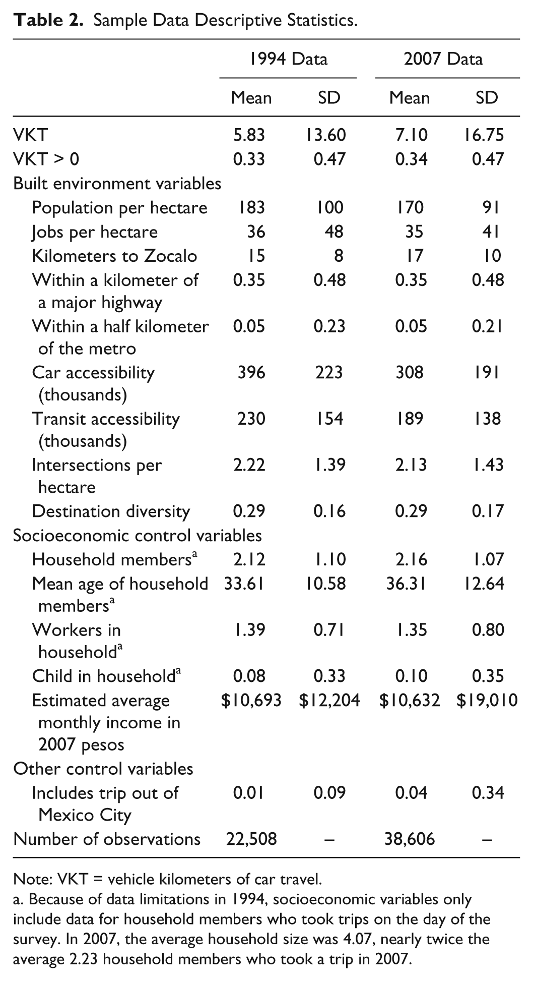
Note: VKT = vehicle kilometers of car travel.
Because of data limitations in 1994, socioeconomic variables only include data for household members who took trips on the day of the survey. In 2007, the average household size was 4.07, nearly twice the average 2.23 household members who took a trip in 2007.
Vehicle kilometers traveled
Vehicle kilometers traveled measures the sum of the total distance traveled in cars divided by the vehicles’ occupancy for all household members older than five. Distances are measured as the network distance between the centroid of each origin and destination’s Census Tract along the road network (see below for a description of the network). The measure does not include trips outside of the metropolitan area, because these destinations’ Census Tract identification numbers were not included in the survey data. One percent of households reported trips that left the metropolis in the 1994 survey, compared with 4 percent in 2007. A dummy variable for trips outside of the metropolitan area is included as a control, since the VKT measure excludes these trips.
Neighborhood population density
Population density measures the total number of people in a household’s home Census Tract divided by the area of the Census Tract in 1990 and 2005. This metric tends to net out major parks, highways, and concentrations of nonresidential land uses, making it closest to a measure of gross residential density. In 2007, the survey captured approximately five thousand Census Tracts, compared to three thousand in 1994. This is the result of new Census Tracts as the metropolis expanded, better coverage in the survey year, and the division of fast-growing Census Tracts.
Job density
Job density measures the total number of jobs in a household’s municipality, divided by the sum of the land area of all urban Census Tracts within the municipality. INEGI (2012) provides job estimates by municipality from the 1998 and 2008 Economic Censuses. These counts were not available at the Census Tract level and exclude jobs without a fixed business location, including informal ones. 4 Density metrics are rescaled in the final models to get the parameter estimates between −1 and 1. This facilitates model convergence and makes the coefficients easier to read. Since job density does not exclude Census Tracts without jobs, it is a grosser measure of density than population density.
Intersection density
Intersection density measures the number of intersections per hectare in each Census Tract. This metric is a proxy for urban design features, since more intersections per acre tend to indicate smaller, more walkable block sizes.
Destination diversity
This index, which relies on survey data about trip purpose and destination, serves as a proxy for land use diversity. Data limitations prevent a more typical land use diversity index. Destinations include eight categories: homes, offices, industrial buildings, schools, retail, hospitals, parks and gymnasiums, and other. A Census Tract’s destination diversity index is
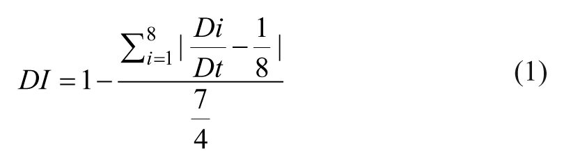
where DI is the diversity index in a given Census Tract, Di is the number of destinations in one of the eight destination categories and Dt is the total number. This specification follows existing work and gives a range of scores from zero, when destinations are only in one category, to one, when there is an equal number of destinations in each category (Bhat and Gossen 2004; Zegras 2010; Rajamani et al. 2003).
Distance to the Zocalo, distance to the metro, and distance to a major highway
All reported distances are the estimated shortest road-network distance from the center of a household’s home Census Tract to the nearest metro or light-rail station point file, highway road segment, or central Zocalo—Mexico City’s historical, geographical, and political center. The same road network is used for the 1994 and 2007 calculations. Although an older road network was available for 1994, this network counterintuitively led to shorter trips, since network calculations assign straight-line Euclidean distances to connect Census Tract centroids and other point files to the road network.
For distance to transit and to the metro, I tested multiple distances before settling on a preferred catchment area (for a description of testing procedures, see Guerra, Cervero, and Tischler 2012). With the preferred distances included, neither the relationship between living within one and two kilometers of a highway nor a half and whole kilometer from a transit station had a statistically significant relationship with VKT generation in 1994 or 2007.
Job accessibility by car and by transit
The job accessibility metric measures the number of jobs accessible by car to a household weighted by a negative exponential decay function for travel time:
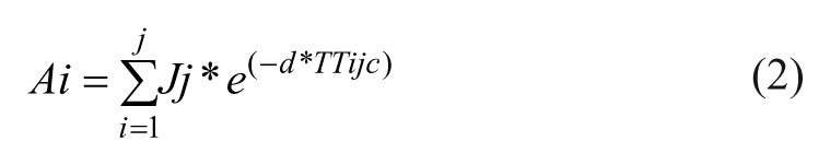
Where Ai is job accessibility in Census Tract i, d is the impedance factor of 0.05, J is the number of jobs in a Census Tract j, and TT is the travel time in minutes between Census Tract i and Census Tract j by car (c).
The final decay function (0.05)—chosen after testing a range from 0.025 to 0.4—gives a job that is 10 minutes away a weight of 61 percent, a job that is 30 minutes away a weight of 22 percent, and a job that is 60 minutes away a weight of 5 percent. The 1994 models fit slightly better with a stronger decay function, while the 2007 models fit slightly better with a weaker decay function. Instead of using the number of formal jobs from above, the accessibility metric uses the total number of job destinations per Census Tract estimated from the household travel survey. Because the surveys were randomized and extrapolated based on household location, measuring jobs in this way likely excludes job destinations from some Census Tracts, while highly overestimating it in others. Unlike for measuring local job density, these errors will tend to cancel each other out over space in a measure of accessibility. I also tested models that included transit accessibility and car accessibility, but dropped transit accessibility because of high levels of multicollinearity as measured by variance inflation scores.
Household income
Average inflation-adjusted income in the sample remained stable across the two time periods, while median income decreased by 8 percent. A reporting difference may influence this result. Only 80 percent of households reported income in 2007, compared to 100 percent in 1994. Nevertheless, the National Household Survey of Income and Expenditures confirms a national 5 percent decline in household income between 1994 and 2006 (INEGI 2011). Although inflation-adjusted GDP per capita increased by 21 percent between 1994 and 2007, adjusted for purchasing power parity, GDP per household declined (World Bank 2012).
Model Forms and Specifications
The discrete decision of whether to drive either precedes or coincides with the more continuous choice of how much to drive. Given a vector of predictor variables (x), a household’s expected VKT (y) is equal to the probability that a household (i) generates any VKT times the expected VKT, if the household produces any:

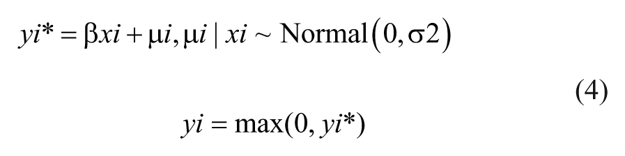
Choosing whether to take any car trips at all is a particularly important choice in Mexico City. Since most households did not generate any VKT on the survey day in 1994 and 2007, ordinary least squares (OLS) regression would produce highly biased estimates of behavior. In particular, it would tend to undervalue the influence of variables that have a strong influence on the choice not to drive at all. To avoid this bias, I estimate standard censored Tobit regression models with left-censoring at zero for 1994 and 2007. The Tobit model jointly estimates whether and how much VKT a household produces as the maximum of zero and a latent variable (y*) that is somewhat akin to a total desired VKT (if for example households could trade VKT for higher income):
Transportation researchers have used this specification—or a variation to correct for selectivity bias when different variables are thought to affect discrete and continuous choices—to model mode choice and distance traveled (Schwanen and Mokhtarian 2005; Golob and van Wissen 1989), mode choice and vehicle travel (Chatman 2003), the ratio of walk and transit trips to drive trips (Greenwald 2003), distances walked (Boarnet, Greenwald, and McMillan 2008), and fuel choice and vehicle travel (van Wissen and Golob 1992).
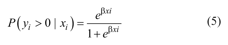
Although the Tobit model provides full information about how VKT and independent variables covary, it may mask important statistical relationships. For example, households in a neighborhood with good accessibility by car are almost certainly more likely to drive than households with poor accessibility. However, they may drive significantly less since destinations are much closer than for households with poor car accessibility. A Tobit model might find no significant correlation between the variables, despite the existence of a strong, but countervailing, correlation with the discrete and continuous decisions. To disentangle possibly confounding correlations, I also estimate logit models of whether households drove on the survey day and OLS regressions of household VKT for the one-third of households that drove. Together, these two models form the first and second half of equation (3):

Because of a long-tailed distribution of household VKT when it is greater than zero, the fitted models estimate the natural log of one plus VKT. This transformation produces a distribution much closer to a normal curve, improves the model fits, and generates more convincingly homoscedastic residual plots.
Testing Changes over Time
In order to evaluate changes in the relationship between VKT and measures of the built environment over time, I pool the two data sets and estimate models with each independent variable interacted with a dummy variable for 1994 and 2007. I then run separate models in which the coefficient for a single built environment variable is constrained to be equal across the two time periods and test whether this improves the overall model fit. In the model results, I only present the final, best-fitting models with constrained and unconstrained parameter estimates.
In the case of the Tobit and logit models, constraining the parameter estimates to be equal improves the model fit, if the unconstrained and constrained models’ log-likelihoods are not statistically different with 95 percent confidence:
where LGLK is a model’s log-likelihood, DF is the degrees of freedom, full is the unconstrained model, con is the constrained model, and χ2* is the critical value on a χ2 distribution that is different from 0 with 95 percent confidence.
For the OLS regressions, model fits are tested using the residual sum of squares (SSE) against a similar critical value on an f distribution (f*):
Prior to testing differences in coefficients, the logit model requires an additional coefficient to rescale all other coefficients for one of the two time periods (Train 2009, chap. 3.2; Ben-Akiva et al. 1994). Since the dependent variable of the logit model is utility—and utility has no absolute value—the size of parameter estimates increases with the variance of the error term. If the error term is larger in one time period than the other, then the parameter estimates will also tend to be larger. The Biogeme software package provides a routine for estimating scalar parameters (Bierlaire 2003, 2009).
Model Results
Table 3 presents the results of the Tobit model predicting the natural log of households’ VKT in 1994 and 2007. While the coefficients have a similar linear relationship to the dependent variable as in an OLS regression, the dependent variable is the uncensored latent variable, rather than actual VKT. Since the dependent variable is the natural log of VKT, the exponent of the coefficient estimates provides an interpretable measure of the relationship between the predictor variables and VKT. For example, a 10-kilometer increase in a household’s distance from the Zocalo correlates with a 0.15 decrease in the natural log of latent VKT. Taking the exponent of this coefficient indicates that a 10-kilometer increase in distance correlates with around a 14 percent decrease in the uncensored latent variable (e−0.15 = 0.86).
Tobit Model Predicting Log of Household VKT Plus One on an Average Weekday in 1994 and 2007.
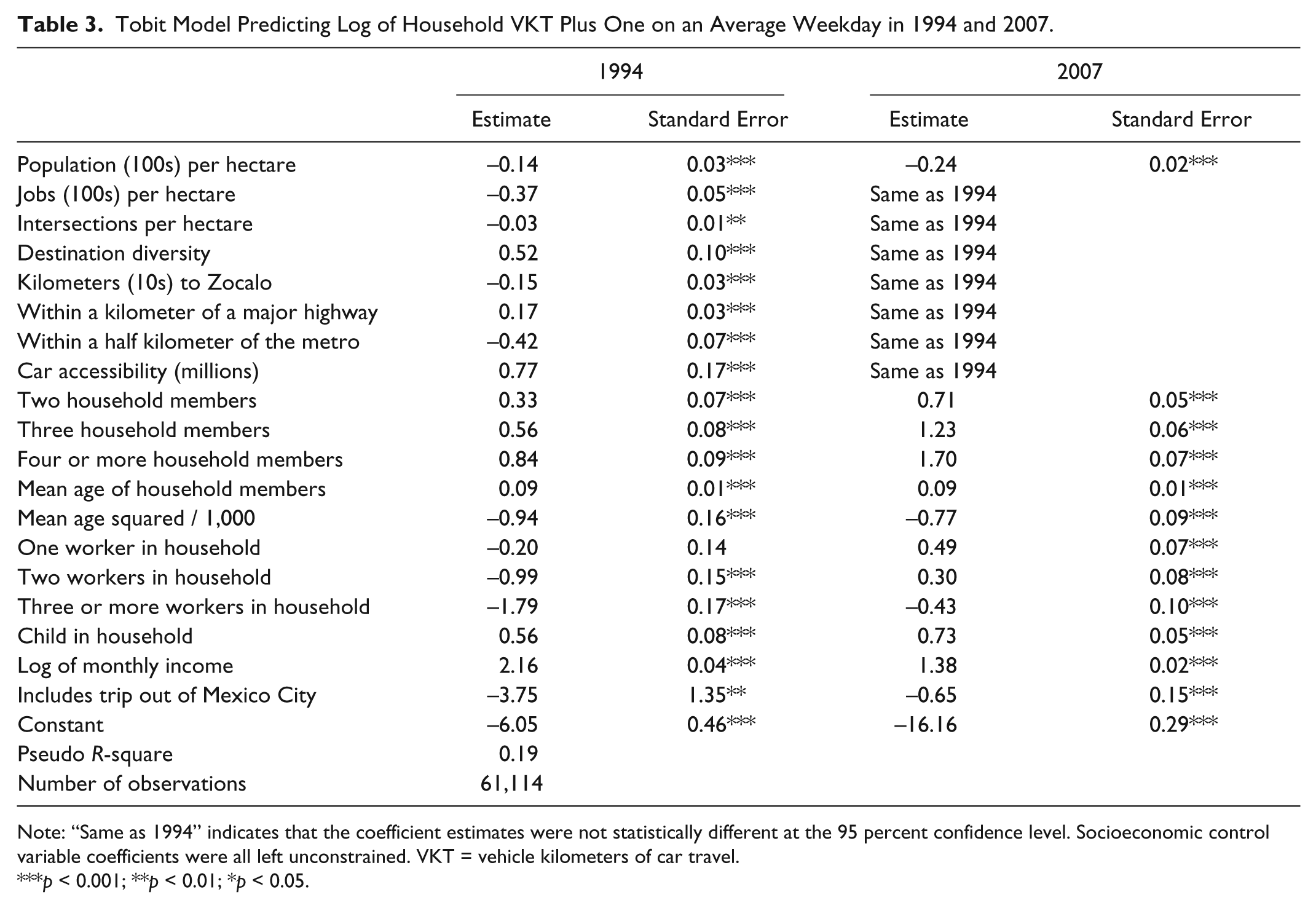
Note: “Same as 1994” indicates that the coefficient estimates were not statistically different at the 95 percent confidence level. Socioeconomic control variable coefficients were all left unconstrained. VKT = vehicle kilometers of car travel.
p < 0.001; **p < 0.01; *p < 0.05.
As expected, higher job and population densities correlate with lower VKT. An additional hundred jobs per hectare predicts approximately 31 percent fewer latent VKT (e−0.37 = 0.69). Higher car accessibility and proximity to highways both were statistically associated with higher VKT, higher intersection density and proximity to the metro, with lower VKT. The statistical relationships conform to the expected influence of density and urban design on VKT. By contrast, higher destination diversity and higher accessibility in a household’s neighborhood associate with higher VKT.
With the exception of population density, none of the measures has a statistically different relationship with VKT across the two time periods (see previous section for a description of the formal statistical tests). One hundred more people per hectare in 2007 correlates with a 21 percent reduction in latent VKT (e−0.24 = 0.79) compared with 13 percent in 1994 (e−0.14 = 0.87). Nevertheless, the coefficients for car accessibility and intersection density in 1994, although not statistically different from the 2007 coefficients, are not statistically different from zero either. All other coefficients, when estimated separately, are statistically significant and move in the same direction across the two periods. 5
The coefficient estimates from the logistic regression of whether a household generated any VKT are quite similar to those from the Tobit model (Table 4). This is unsurprising since two-thirds of households in the sample reported no VKT. As with the Tobit model of the natural log of VKT, taking the exponent of coefficients from the logistic regression provides more easily interpreted results. For example, increasing the number of jobs per hectare by one hundred decreases the odds that a household produces any VKT by around 17 percent (e−0.19 = 0.83). The odds ratio of 1.09 derived from taking the exponent of the coefficient 0.09 indicates that being within a kilometer of a highway correlates with 9 percent higher odds that a household generates any VKT. The relationship between intersection density and whether a household generates VKT moves in the expected direction, but is not statistically different from zero. Again, a marginal change in population density is correlated with a lower probability of driving in 2007 than in 1994. Car accessibility also has a significantly stronger correlation with car use in 2007 than in 1994.
Binomial Logit Model Predicting Whether VKT Is Greater Than Zero.
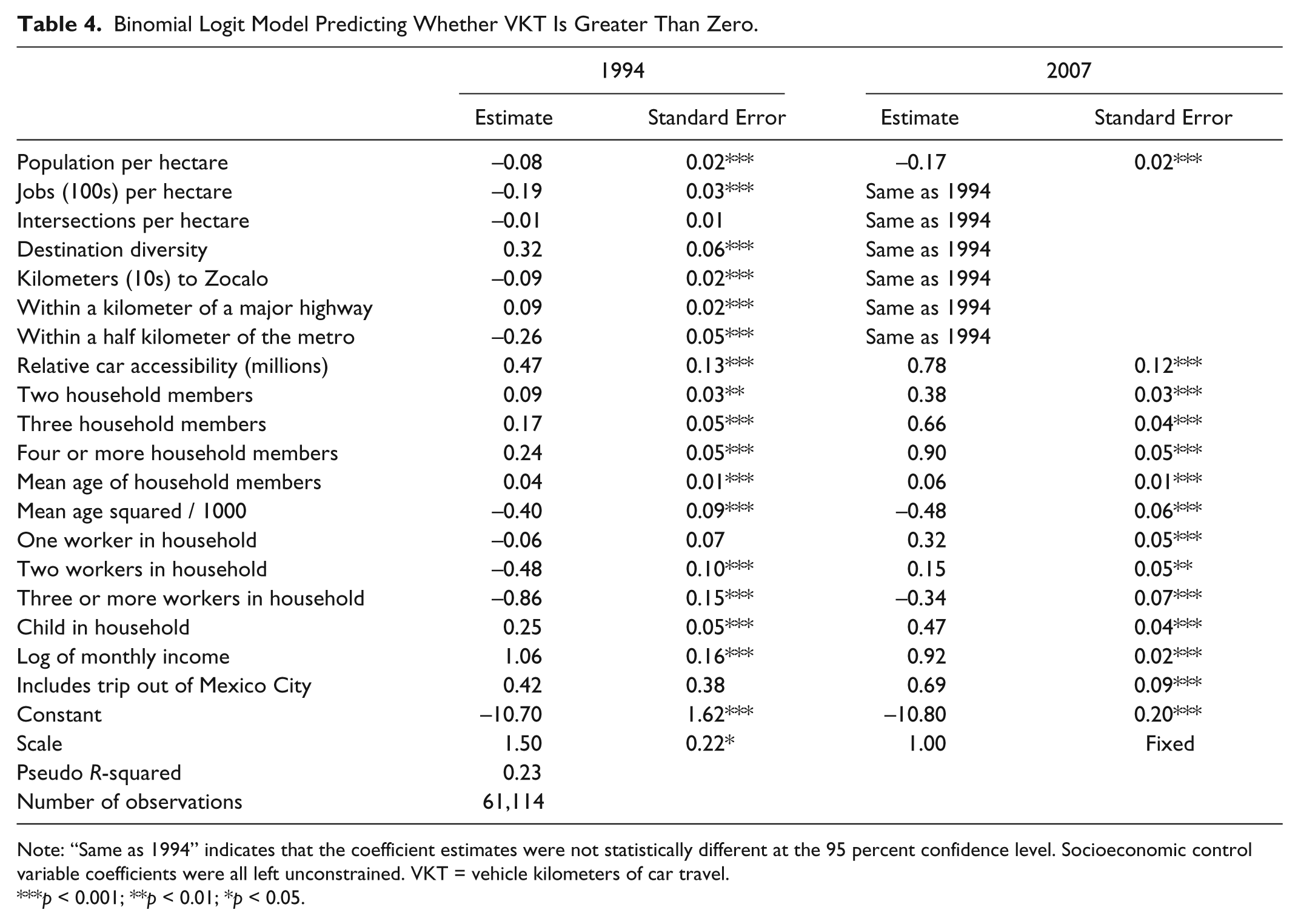
Note: “Same as 1994” indicates that the coefficient estimates were not statistically different at the 95 percent confidence level. Socioeconomic control variable coefficients were all left unconstrained. VKT = vehicle kilometers of car travel.
p < 0.001; **p < 0.01; *p < 0.05.
As previously discussed, pooling data and estimating a logistic regression for the two time periods requires the estimation of a scalar variable to ensure comparable coefficient estimates. The estimated scale is statistically significant and greater than one, indicating greater variation in the error term in 1994. This suggests more variation in unobserved attributes, such as personal preference, or possibly less reliable data in that year.
For the one-third of households that reported VKT in the surveys, the correlations between the built environment variables and total VKT tend to be weaker than in the Tobit or logit models (Table 5). For example, a one hundred person increase in people per hectare correlated with 3 percent fewer VKT, compared with a 13 percent to 21 percent decrease in latent VKT in the Tobit model. Jobs and intersections per hectare are statistically associated with fewer VKT at the 90 percent confidence level but not the 95 percent level. In addition to a general weakening of the statistical relationships, two coefficient estimates change signs. The subset of households that generate VKT in the two time periods generate statistically more VKT in areas with poor car accessibility and homogenous destination types. It appears that households in diverse, accessible neighborhoods are more likely to drive, but drive shorter distances than they would in single-use, inaccessible neighborhoods.
OLS of the Natural Log of VKT Plus One for Households with VKT Greater Than Zero.
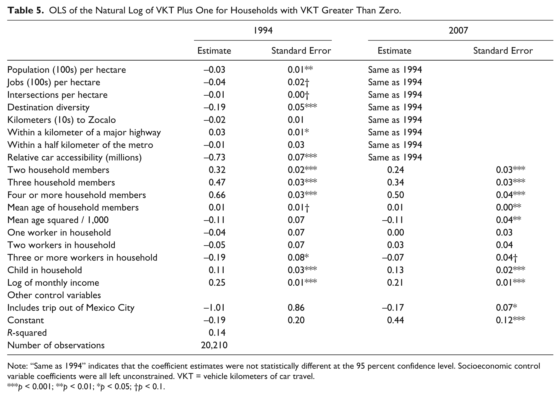
Note: “Same as 1994” indicates that the coefficient estimates were not statistically different at the 95 percent confidence level. Socioeconomic control variable coefficients were all left unconstrained. VKT = vehicle kilometers of car travel.
p < 0.001; **p < 0.01; *p < 0.05; †p < 0.1.
Limitations
In addition to general caveats about data and causal inference, three issues of sample selection may bias the results. First, the surveys exclude pedestrian trips and—because of a data limitation in 1994—non-trip-making households. In 2007, 15 percent of all surveyed households did not report a vehicular trip on the survey day. Presumably they took no trips, took only pedestrian trips, or failed to report vehicular trips. As a result, the models are biased toward the behavior of households taking vehicular trips. Using the full 2007 data sample, I find that models excluding non-trip-taking households produce slightly smaller parameter estimates than models including them, but larger elasticity estimates, because of the higher proportion of nondriving households in the sample.
Second, the Tobit model of VKT is unavoidably biased toward the behavior of the one-third of households that reported generating positive VKT in the 1994 and 2007 samples. Their recorded attributes factor into the estimation of the probability that a household generates VKT as well as the amount generated. Since these households likely differ systematically from the total population sample in ways that cannot be statistically controlled—for example, they may have an unmeasured preference for driving—their driving habits may be less sensitive to marginal changes in income, the built environment, or household composition. Nevertheless, the stability in coefficient estimates between the 1994 and 2007 sample, despite changes in the proportion of households generating VKT, indicates that the estimated relationships tend to hold, at least for those households at the margin of choosing to generate VKT.
Third, this analysis does not correct for residential self-selection. As Brownstone (2008, 2) puts it, “The observed correlations between higher density and lower VMT may just be due to the fact that people who choose to live in higher density neighborhoods are also those that prefer lower VMT and more transit or non-motorized travel.” Mokhtarian and Cao (2008) and Cao, Mokhtarian, and Handy (2009) identify nine methodologies to address residential self-selection, summarize the findings from 38 studies that use them, and conclude that failing to account for residential self-selection tends to lead to overestimates of the relationship between the built environment and travel. Chatman (2009), however, finds that failing to account for self-selection can produce underestimates, as well as overestimates. Furthermore, the built environment likely influences preferences that, in turn, influences residential selection (Weinberger and Goetzke 2010). Brownstone and Golob (2009) and Bhat and Guo (2007) find that including a rich set of sociodemographic control variables—as this study does—appears to account for most, if not all, residential self-selection. Nevertheless, the failure to account for residential self-selection is an undoubted limitation.
Discussion
Contrary to expectations, the estimated relationship between the built environment and daily VKT is fairly stable, though modestly stronger over time. Of the eight metrics analyzed, only population density has a statistically different correlation with total VKT across the 1994 and 2007 surveys. The results suggest that a one unit increase in population density had nearly twice the constraining effect on VKT in 2007 as in 1994. Furthermore, car accessibility and intersection density are statistically significantly correlated with VKT in 2007 but not in 1994. In this respect, the relationship between VKT and the built environment also appears stronger over time. In the logit model of whether a household generated any VKT, the relationships with population density and car accessibility are also stronger in 2007 than in 1994. Intersection density is not statistically correlated with whether a household generates VKT in either year. For the one-third of households that generated VKT, none of the estimated coefficients for measures of the built environment differ across the two time periods. However, these correlations are generally weaker and less statistically significant. Taken together, the results from the three models suggest that the built environment has an increasingly important role to play in constraining or encouraging car use in Mexico City.
To compare results with those from other studies and better understand the relationship across the three models, Table 6 provides elasticity estimates of the relationship between VKT and the eight measures of the built environment in 1994 and 2007 from the Tobit, logit, and OLS models. If a coefficient estimate is not statistically different from zero with at least 90 percent confidence, the elasticity is not reported. Given nonlinearity in the estimation procedures, directly estimating elasticities from the regression outputs likely produces biased results (Train 2009, 30). Instead, the reported elasticities represent the average response of each household to a change in one of the built environment variables across the population. For dummy variables that cannot be increased marginally, such as whether a household lives within a half kilometer of the metro, households with a value of zero are randomly assigned a positive value in order to estimate elasticities.
Elasticity of Car Use with Respect to Changes in the Built Environment.
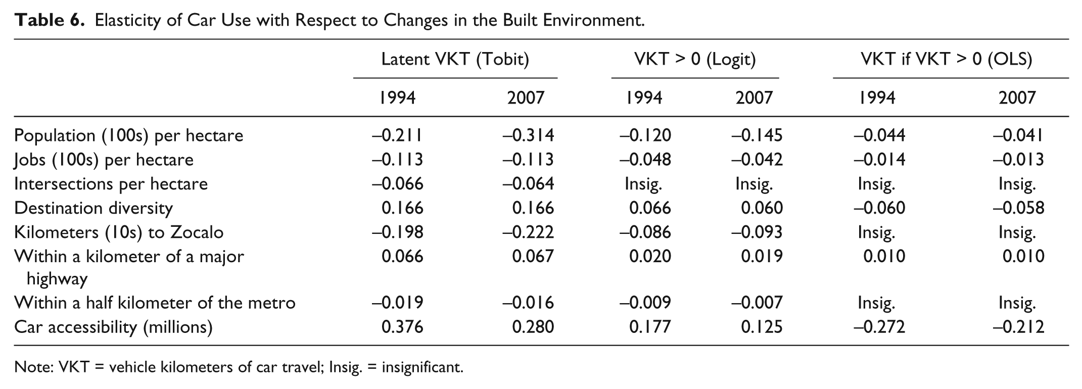
Note: VKT = vehicle kilometers of car travel; Insig. = insignificant.
In the case of the Tobit models, the elasticity relates to the relationship between the built environment and latent predicted VKT. While it is possible to estimate the relationship between the built environment variables and total VKT, this produces estimates that are biased toward the behavior of the households with the highest predicted VKT. Given that the predicted log transformation of VKT ranges from negative to positive seven, this bias is substantial. At an estimated value of seven or negative seven, the proportional change in an individual household’s estimated latent VKT due to a change in a given predictor variable is identical. The difference in predicted VKT, however, is quite substantial. For example, at a predicted value of seven, a one unit increase in millions of accessible jobs equates with 1,272 additional VKT. At negative seven, there is no predicted change since the Tobit model continues to predict a negative value. Furthermore, it is not possible to calculate elasticities for individual households that move from zero to positive VKT. I therefore opt to report elasticities for latent rather than actual VKT. The estimated elasticities for total VKT (rather than latent VKT) are smaller for variables that correlate with lower VKT and larger for variables that correlate with higher VKT, because of the bias.
For the one-third of households that generated VKT, the estimated elasticities of VKT with respect to population density, car accessibility, and destination diversity are strikingly similar to the weighted average elasticities of studies reported by Ewing and Cervero (2010, 273). The relationship with job density is stronger, but within the range of the six studies used to estimate the weighted average elasticity. Intersection density and proximity to transit are also within the range of reported elasticities, though neither is significantly correlated with VKT. The relationship between VKT and distance to the downtown is much weaker than the range of elasticities (−0.18 to −0.27) reported by Ewing and Cervero. However, distance to the downtown is generally included as a proxy for accessibility. None of the cited studies included both distance to the downtown and a measure of accessibility.
By contrast, the correlation between measures of the built environment and whether a household produces any VKT is two to ten times stronger. For example, a doubling of a neighborhood’s population density corresponds on average to a 12 to 15 percent decrease in the number of households that drive but only a 4 percent reduction in driving households’ VKT. Gross population density, while an increasingly important disincentive to driving, has a weak and constant relationship with VKT once a household generates at least some VKT. The relationship with latent VKT combines the predicted influence on whether and how much households drive and is even stronger at −21 percent in 1994 and −31 percent in 2007. Job density and proximity to highways and transit also have a much stronger correlation with whether a household generates VKT on a given weekday than how much it generates.
More interestingly, the estimated relationships between the built environment and whether and how much households drive do not always move in the same direction. Households that live in urban areas with good car accessibility and diverse destinations are more likely to drive than similar households in less accessible and diverse, suburban neighborhoods. Once a household generates VKT, however, it generates significantly more in the areas with poor car accessibility and undiversified destinations. For example, a doubling of a household’s neighborhood’s destination diversity correlates with a 6 percent higher probability of driving but 6 percent fewer VKT for the households that do drive. Presumably, this is because they have to drive longer distances to fulfill daily activities.
Conclusion
After controlling for income and other household attributes, population and job density, transit and highway proximity, destination diversity, and intersection density are statistically correlated with car travel in Mexico City. Across the 1994 and 2007 data, the estimated correlations are fairly stable. Where they have changed, they strengthened over time. While the magnitude of the relationships between car use and most measures of the built environment are similar to those found in U.S. cities for the subset of households that drive on an average weekday in Mexico City, they are stronger when all households are included. To the extent that relationships are causal, this is good news for the civil society groups and planners promoting land use planning to constrain car travel. Not only does the relationship appear to be somewhat stronger than in the United States, it also appears to be strengthening. As in the United States, however, no individual measure of the built environment has more than a moderate correlation with VKT: elasticities range from −0.31 to 0.38. This is far weaker than the relationship to household income, a doubling of which correlates with two to three times more latent VKT. This suggests that—as in U.S. cities—land use planning can play a role in reducing car travel, but that the effects will likely be modest unless done in concert with travel demand management, transit investments, and other supportive policies.
In addition to supporting common planning practices such as encouraging development around transit stations, limiting highway expansion, and increasing or maintaining local densities, the findings have two less commonly referenced implications for policy makers concerned with slowing the growth of car use in Mexico City. First, if indeed the built environment influences travel behavior in Mexico City, most of this influence occurs through households’ decisions of whether, rather than how much, to drive. This suggests that land use policies will have a stronger impact on VKT when directed at neighborhoods with low-to-average, rather than high, driving rates. If most households in a neighborhood drive—whether due to preference, higher wealth, or other factors—they will be far less responsive to physical changes in the neighborhood than those residing in a neighborhood where more households are at the margin of choosing to drive. It also suggests more generally that policies designed to reduce the likelihood that households drive on an average day are likelier to bear fruit than policies designed to reduce the amount that they drive. For example, policies to encourage suburban job accessibility—while potentially meritorious for other reasons—would tend to decrease VKT for driving households, but increase total VKT, by encouraging a shift to cars from other modes. Though not directly measured in this study, maintaining and improving viable alternatives to car travel appears to be critical. In Mexico City, this almost certainly means increasing the attractiveness of public transportation, which carried 71 percent of non-pedestrian trips in 1994 and 62 percent in 2007.
Second, households in low-diversity, inaccessible neighborhoods are among the least likely to drive, but once they drive, they tend to drive a lot. Given the rapid increase in population and driving rates in peripheral neighborhoods that are far from job centers, this is worrying. Eighty-five percent of the 8.3-million-kilometer increase in weekday car travel between 1994 and 2007 occurred outside of the Federal District. In order to slow the increase in VKT, policy makers would do well to target policy toward inaccessible neighborhoods with low driving rates but a high potential for generating significant VKT. In these peripheral neighborhoods that are far from the existing metro system, informal transit is the car’s chief and often only competitor. Unless the government or private sector can quickly extend high-capacity transit to these neighborhoods or reorient growth patterns away from the periphery, improving informal transit should be a key transportation policy goal. If these residents start driving, land use planning will likely have a much smaller influence on how much they drive.
Footnotes
Acknowledgements
The research and text have benefited greatly from comments from Robert Cervero, Joan Walker, Dan Chatman, Elizabeth Deakin, David Hsu, Megan Ryerson, Rebecca Sanders, Allie Thomas, Jake Wegmann, and three anonymous reviewers. I would also like to thank Salvador Herrera and CTS-EMBARQ for support and assistance in Mexico City.
Declaration of Conflicting Interests
The author declared no potential conflicts of interest with respect to the research, authorship, and/or publication of this article.
Funding
The author disclosed receipt of the following financial support for the research, authorship, and/or publication of this article: A University of California Transportation Center Dissertation Grant and a Dean’s Normative Time Fellowship from the University of California Berkeley’s Graduate Division.