
Abstract
The Wechsler Intelligence Scale for Children-Fifth Edition (WISC-V; Wechsler, 2014) provides a general intelligence score, representing g, and five index scores, reflecting underlying broad factors. Within person differences between the overall performance across subtests and index scores, denoted as index difference scores, are often used to examine profiles of strengths and weaknesses. In this study, the validity of such profiles was examined for the Dutch WISC-V. In line with previous studies, broad factors explained little variance in index scores. A simulation study showed that variation in index difference scores also reflected little broad factor variance. The simulation study further revealed that, as a consequence, a significant discrepancy between an index score and overall performance was accompanied in only 40%–74% of the cases by a discrepancy on the underlying broad factor. Overall, these results provide little support for the validity and thereby clinical use of WISC-V profiles.
Intelligence is probably the most widely assessed ability around the world (Evers et al., 2012). In children it is used to inform a range of educational decisions including eligibility for special services, placement in secondary education, underperformance in the classroom and the diagnosis of several developmental disorders that are relevant in the context of school (Benson et al., 2020).
Intelligence scores or IQ scores are usually determined with a battery of (sub)tests. Additionally, variation in performance across subtests or composites of subtest [i.e. profiles of strengths and weaknesses] are often considered (Kranzler et al., 2020). However, the clinical use of such profiles has been hotly debated for many years. Some have argued that further scrutiny of a profile, like a ‘detective’ (Kaufman, 1994), can provide additional information that is relevant to understanding an individual’s intellectual functioning and needs for treatment. Others have questioned the reliability, stability and validity of such profiles (Macmann & Barnett, 1997; McGill et al., 2018; Watkins & Canivez, 2004), and tried to debunk the ‘myth of the master detective’ (Macmann & Barnett, 1997) or advised to ‘just say no to subtest analysis’ (McDermott et al., 1990). The release of the fifth edition of the Wechsler Intelligence Scale for Children (WISC-V) seems to have given a new impetus to this debate (Canivez et al., 2017; Dombrowski et al., 2018; McGill et al., 2018). In this study, I consider the validity of profiles of strengths and weaknesses on the basis of the Dutch version of the WISC-V (Wechsler, 2018).
The WISC-V is based on the Cattell-Horn-Carroll model (CHC-model) of cognitive abilities, which McGrew (2009) claims to be the most encompassing taxonomy of cognitive abilities. The CHC-model resulted from merging the Cattell-Horn model with Carroll’s Three Stratum model, two models of the structure of cognitive abilities which are often regarded as similar although only the latter model includes g (Canivez & Youngstrom, 2019). The CHC model is a hierarchical model with a general factor at the highest level affecting approximately 16 broad abilities at a second level, which in turn each affect a range of specific cognitive abilities at the lowest level.
The WISC-V consists of 16 subtests that are assumed to measure g, and five broad abilities of the CHC model: Verbal Comprehension, Visual Spatial, Fluid Reasoning, Working Memory and Processing Speed. The major scores are derived from only 10 subtests; a Full Scale IQ (FSIQ) based on seven subtests and the General Index Score (GIS-index) based on 10 subtests. In addition, five index scores can be derived, each based on two of the subtests. The index scores are presumed to reflect the five broad abilities. Furthermore, index difference scores can be computed by subtracting the GIS-index (or FSIQ) from an index score. A significant discrepancy between an index score and the GIS-index (or FSIQ) indicates a strength in case the index score is higher than the GIS-index, or a weakness, in case the index score is lower (Wechsler, 2014; 2018).
Structure of the WISC-V
In a number of studies Canivez and colleagues have addressed several problems with the interpretation of the five index scores (Canivez et al., 2017; Canivez, et al., 2018; Dombrowski et al., 2015; 2018; 2022; Watkins & Canivez, 2022). One problem concerns the factor structure of the WISC-V. The appropriateness of the five factor model is important as it underlies the index scores which form the basis for the interpretation of strengths and weaknesses in cognitive abilities. The five factor model reported in the technical manual of the American version has redundancies as shown by re-analyses of data (e.g., Dombrowski et al., 2015; Dombrowski et al., 2019) as well as by a simulation study (Dombrowski, et al., 2021). For example, the second order g factor and the broad factor Fluid Reasoning are identical and the model implied correlation of Fluid Reasoning with Visual Spatial is .88. In a series of studies Canivez and colleagues showed that a model with four broad factors provides a better and more parsimonious description of the 16 subtests as well as the 10 primary subtests of the US version of the WISC-V (Canivez, et al., 2016; 2017; Dombrowski, et al., 2018; Dombrowski et al., 2019). In their four factor solutions, the Visual-Spatial and Fluid Reasoning factors merged together. Similar results were reported for the French and the German version of the WISC-V (Lecerf & Canivez, 2018; Pauls & Daseking, 2021
Another problem with the validity of the index scores, mentioned by Canivez and colleagues, concerns the extent to which these scores reflect the underlying broad factor. This problem is considered in the present study for the scores of the Dutch version of the WISC-V. In addition, also the validity of the index difference scores is examined as these scores form the basis of profiles of strengths and weaknesses.
Validity of Index Scores
Canivez and colleagues have repeatedly highlighted the limited amount of variance in the index scores that can be attributed to the associated underlying broad factor, denoted here as the lack of validity of the index scores (e.g., Canivez et al., 2017; McGill et al., 2018; Watkins & Canivez, 2022). Most of the variance of an index score is accounted for by the g factor and not by the broad factor that it is presumed to reflect. A review by McGill et al. (2018) shows that the broad factors on average account for less than 25% of the variance, with the processing speed index at one extreme (18%–52%) and fluid reasoning at the other (0%–6.6%). Therefore, Canivez and colleagues have concluded that the index scores of the WISC-V are of questionable value for clinical decisions (Canivez et al., 2017; Watkins & Canivez, 2022).
Most studies on the (un)interpretability of WISC-V index scores have followed the logic of factor analysis and decomposed the variance of the index scores into three independent sources: the g factor, the broad factor and unique variance. But for a particular subtest, the unique variance consists of measurement error and specific variance. Measurement error indicates the unreliability of the subtest. The specific variance of a test reflects one or more additional abilities that are required for a particular subtest but are unrelated to the specific abilities needed for the other subtest associated with the index (Brunner et al., 2012; Schneider, 2013). The specific abilities of both subtests are also a source of variance for the index score. Usually, these specific abilities are assumed to reflect very specific, and mostly uninteresting, features of the task. In some cases, however, there might be a substantive interpretation of the subtest-specific variance. For example, the working memory index is determined by two span tasks, Digit Span and Picture Span. These task probably (partly) represent different aspects of the working memory system (Baddeley, 2012), with Digit Span depending more on the verbal subsystem and Picture Span more on the visual-spatial subsystem. Thus, the amount of task specific variance in the index scores can be of interest, but is still largely unknown.
Validity of Index Difference Scores
As said, a strength or weakness on an index does not concern the index score as such, but a difference between an index score and the GIS-index (or FSIQ). Accordingly, an important question in the use of profiles is the extent to which index difference scores actually reflect the underlying broad factor. At first sight these difference index scores might fare better than the index scores because these difference scores are corrected for the influence of the g factor. However, two caveats should be mentioned. First, the absence of the g factor in a difference index score comes at a cost, as difference scores can be unreliable and will certainly be less reliable than the index scores (Cronbach & Furby, 1970; Watkins & Canivez, 2022). Second, there is a relation between the sources of variance in the index and the index difference score. That is, the amount of broad factor variance in an index score affects the amount of broad factor variance in an index difference score. However, how a lack of broad factor variance in an index score affects the amount of variance accounted for by the broad factor in the index difference scores of the WISC-V is not yet known. It is also unclear to what extent these difference index scores reflect other sources of variance, such as subtest specific factors.
Even if an index difference score reflects an insufficient amount of variance of the underlying broad factor, the meaning of such an outcome remains somewhat elusive. Knowledge of the amount of such variance might not clarify the relation between an observed discrepancy (strength or weakness) and the likelihood of a discrepancy of similar magnitude on an underlying factor. Put differently, for practitioners it seems more apt to ask how often a significant weakness or strength on an index score can be attributed to a weakness or strength on the broad factor and/or to the specific factors that are believed to underlie a particular index score.
Current Study
The main aim of the current study was to examine the validity of the index and index difference scores of the Dutch WISC-V. With respect to the five index scores, the amounts of variance accounted for by the various sources, that is the g factor, the broad factor and the specific factors, were derived from the five factor solution as reported in the technical manual (Wechsler, 2018). To put these amounts of variance into perspective, they were compared to the variance described by these sources in the US version of the WISC-V (Wechsler, 2014). Following previous studies, it was expected that most of the variance in the index scores is accounted for by the g factor, with smaller contributions of the broad factor and the specific factors. Next, the validity of the five index difference scores was assessed through a simulation study. The amount of variance captured by the broad and specific factors was expected to be somewhat higher in the difference scores than in the index scores, as the index difference scores do not reflect the g factor. The data of the simulation study were also used to examine how often a weakness or strength on an index score, that is a significant positive or negative index difference score, was accompanied by a similar weakness or strength on the underlying broad factor.
Method
Variance Decomposition of Index Scores
Computation of the contributions of variance by the various sources underlying the index scores was based on Figure 1 for the Dutch WISC-V and on Dombrowski et al. (2018, Figure 1, p. 92) for the US WISC-V. The reliabilities of the primary subtests came from the Dutch and US technical manuals (Wechsler, 2014, 2018). Hierarchical factors model of the Dutch WISC-V with standardized coefficients (information taken from Figure 6.2 in Wechsler [2018]). SI = Similarities, VC = Vocabulary, BD = Block Design, VP = Visual Puzzles, MR = Matrix Reasoning, FW = Figure Weights, DS = Digit Span, PS = Picture Span, CD = Coding, SS = Symbol Search.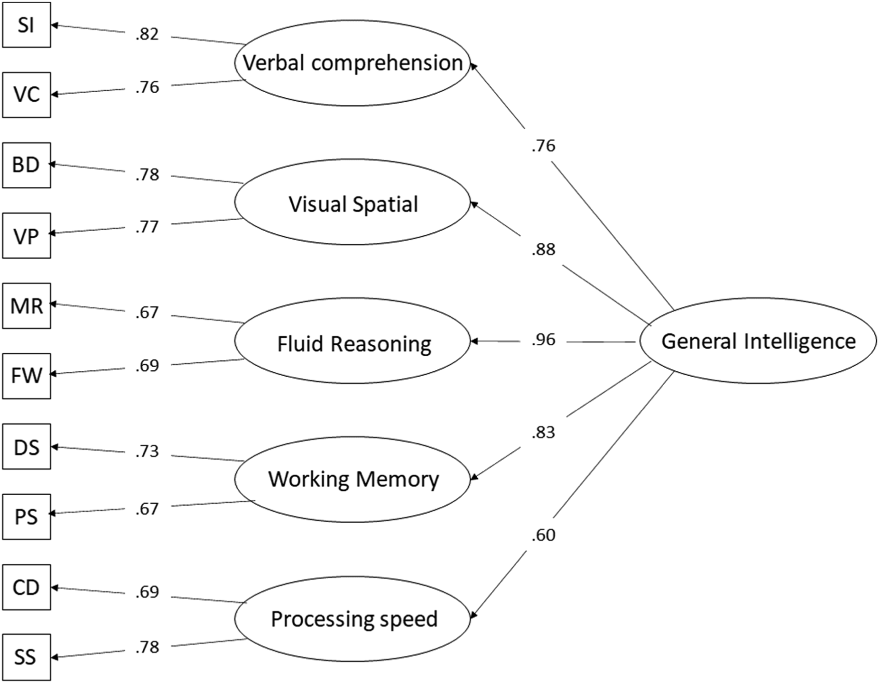
Variance decomposition of the index scores comprised two steps. First, the variance of each subtest was decomposed into variance accounted for by the g factor, variance accounted for by the broad factor, error variance and specific variance. The proportion of variance accounted for by the g factor was computed by multiplying the factor loading of a subtest on its broad factor by the factor loading of the broad factor on the g factor and then taking the square root of this product (Brunner et al., 2012). The proportion of variance contributed by the broad factor after the g factor variance was accounted for, was computed by subtracting the g factor variance from the square of the factor loading of the subtest on the broad factor. The proportion of error variance due to measurement error was obtained by subtracting the reliability of the subtest as reported in the technical manual from one. Finally, the proportion of specific variance was computed by subtracting the proportion of error variance from the residual subtest variance, which was computed by subtracting the squared loading of the test on the broad factor from one.
In the second step the total variance of an index score was decomposed. Coefficient Omega hierarchical scale was used to compute the unique proportion of variance that each of the factors (g factor, broad factor, specific factors and errors) accounted for in the variance of the index score (Brunner et al., 2012; Reise, 2012). Although, Omega hierarchical scale is usually considered a reliability estimate of a scale, it essentially expresses the amount of variance described by one source of variance divided by the total amount of variance described by all sources of variance of a score, in this case an index score. The computations were based on an adaptation of Formula 3 in Brunner et al. (2012, p. 825). The adaptation was to split the residual variance ei into (test) specific variance si and measurement error εi (see Appendix A). For valid clinical interpretation of an index score, Omega hierarchical scale for the broad factor should be at a minimum of .50, but .75 is to be preferred (Reise et al., 2013).
Variance Decomposition of Index Difference Scores
Simulation Procedure
Following the logic of the hierarchical factor model in Figure 1, each subtest can be decomposed into four independent factors: The g factor, the broad factor, the specific factor and an error factor. The full factor model of the 10 primary subtest consists of 26 independent variables: One g factor, 5 broad factors, 10 specific factors and 10 error factors. The R program (R Development Core Team, 2016) was used to generate a sample of 1,000,000 cases from a multivariate normal distribution of 26 independent variables with a mean of zero and a variance of one (Beaujean, 2018; Miciak et al., 2018). The code for the simulation is listed in Appendix B.
Generated scores were not transformed, and were not rounded to whole numbers. The z-score metric was used in all analyses because a) sources of variance in the difference scores are not dependent on metric and b) the use of the z-score metric will not affect the conclusions that follow from the results.
For each case, subtest scores were computed as the weighted sum of the underlying factors of the subtest, that is the general factor, the broad factor involved in the subtest, its specific factor and its error factor. The weights were the square root of the proportions of variance accounted for in a particular subtest (see section Validity of index scores above). For a particular subtest, these weights are identical to the factor loadings of the subtest on its underlying factors. Then, the index scores were computed as the average of the two subtest scores and the GIS index as the average of the 10 primary subtests. Finally, five index difference scores were computed by subtracting the GIS index from each index score.
Sources of Variance in Index Difference Scores
To determine the sources of variance in the five index difference scores, each of these scores was regressed on the assumed underlying sources of variance of the index. Each difference index score was regressed on seven types of factors. Four factors were related to the particular index score: 1) the g factor, 2) the broad factor that the index score is assumed to reflect, 3) the subtest specific variance of the two subtests that are the basis of the index, and 4) the errors of these two subtests. Three types of factors were unrelated to the particular index, that is all other 1) broad factors (4 in total), 2) test specific factors (8 in total) and 3) subtest errors (8 in total). Together, proprotions of variance of all related and unrelated underlying factors add up to one.
The factors were subsequently added to the regression model to determine the change in R 2 . This change indicated how much variance a particular type of factor added. Note that the particular order of inclusion of the factors was irrelevant, because all factors were independent, that is, had a correlation of zero, which is a consequence of the assumption underlying the factor model of the tests.
Classification Procedure of Observed and Underlying Weaknesses or Strengths
The data of the simulation study were also used to examine the relation between an observed discrepancy on an index score and discrepancies on the underlying factors of the index difference score. The classification of cases with and without a discrepancy between the index score and the GIS index was based on the index difference scores. Note that a discrepant index score means that the index difference score differs significantly from zero. Cut-off scores for discrepancies depended on the significance level of the difference between index and GIS-index. In the current study, significance levels of .05 and .01 were examined. The cut-off score that belongs to each level of significance of each particular index score was derived from the technical manual (Wechsler, 2018). The discrepancies between the GIS-index and an index score in z-scores ranged from 0.68 to 0.75 at an alpha level of .05 and from 0.81 to 0.90 at an alpha level of .01.
Next, cases with and without discrepancies on the underlying factors of the difference index scores, that is the broad factor, two test specific factors and two errors, were distinguished. Discrepancies on these five underlying factors were based on the same z-score cut-offs used to determine a discrepancy (strength or weakness) on an index score. There are 32 possible combinations of discrepancies on the five underlying factors. Three broader categories were considered: 1) The percentage of cases with an underlying discrepancy on the broad factor, 2) the percentage of cases with a discrepancy on one or both task specific factors only and 3) the percentage of cases with discrepancies on one or both errors only. The remaining possibilities concerned discrepancies on combinations of task specific and error factors which are difficult to interpret and were therefore lumped into the category ‘other’. The computations were done separately for strengths and weaknesses.
Results
The results are presented in three sections. The first two sections contain the results on the sources of variance in the index and index differences scores, respectively. The last section presents the results on the relation between observed strengths and weaknesses on index scores and the discrepancies on the factors that underlie the index difference scores.
Sources of Variance in the Index Scores
Proportion of Variance per Source for each of the 10 Subtests of the Dutch and US WISC-V.
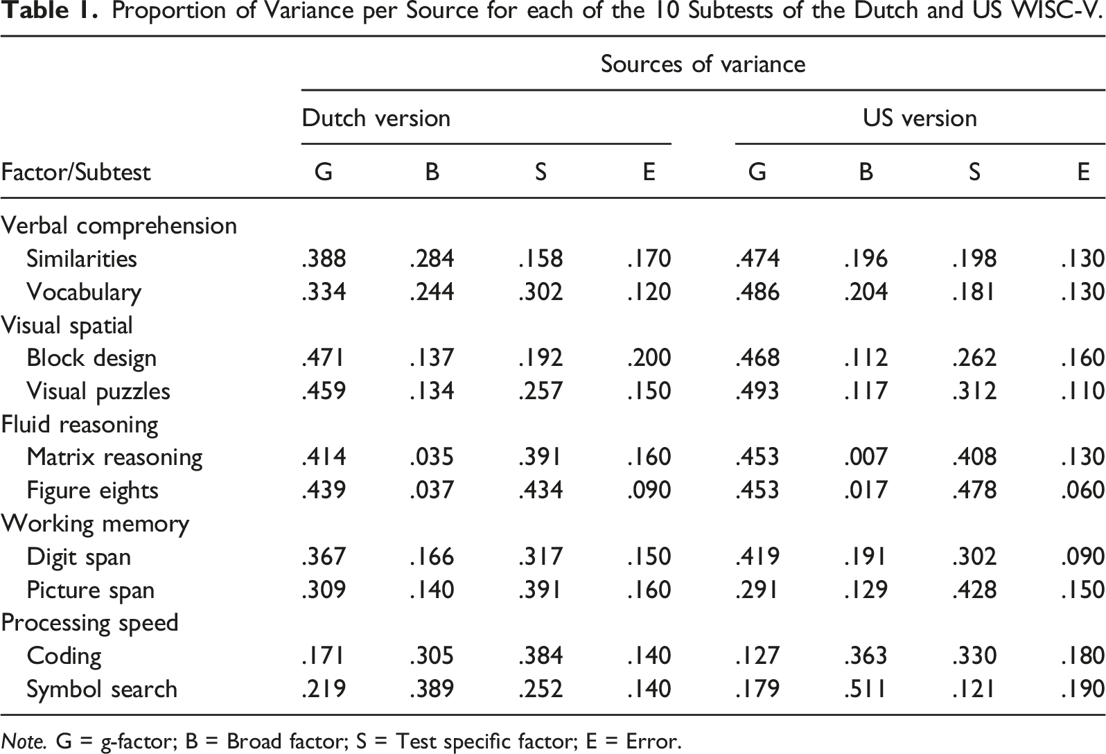
Note. G = g-factor; B = Broad factor; S = Test specific factor; E = Error.
Proportion of Variance per Source per Index and General Score for the Dutch and US WISC-V.
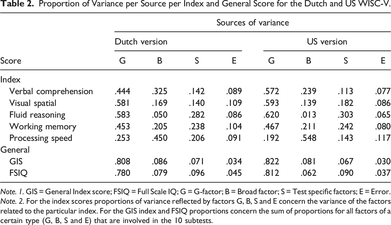
Note. 1. GIS = General Index score; FSIQ = Full Scale IQ; G = G-factor; B = Broad factor; S = Test specific factors; E = Error.
Note. 2. For the index scores proportions of variance reflected by factors G, B, S and E concern the variance of the factors related to the particular index. For the GIS index and FSIQ proportions concern the sum of proportions for all factors of a certain type (G, B, S and E) that are involved in the 10 subtests.
Sources of Variance in the Index Difference Scores
The sources of variance of the index difference scores were derived from the simulated data. First, however, the quality of these data was examined. To this end, in the simulated data, each of the index scores was regressed on its underlying sources of variance. Regression analyses were also conducted for the FSIQ and the GIS index. The outcomes of these regression analyses were compared to the Omega hierarchical scale values reported for the Dutch version of the WISC-V in Table 2. The results were virtually identical. A very small difference, ranging from .001 to .003, was found for 7 out of the 28 proportions.
Proportion of Variance per Source per Difference Index score for the Dutch WISC-V.
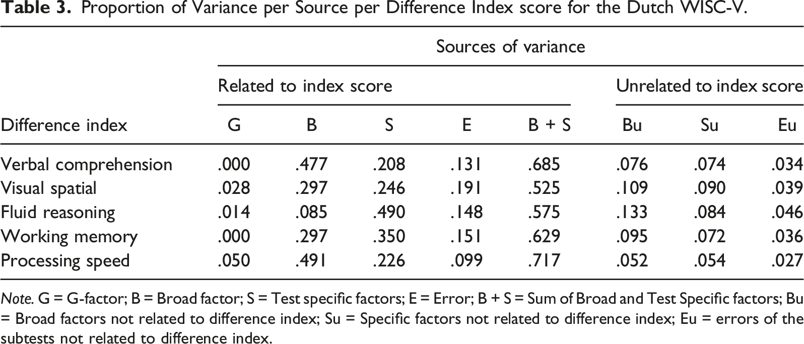
Note. G = G-factor; B = Broad factor; S = Test specific factors; E = Error; B + S = Sum of Broad and Test Specific factors; Bu = Broad factors not related to difference index; Su = Specific factors not related to difference index; Eu = errors of the subtests not related to difference index.
As expected, the g factor accounted for negligible amounts of variance. The amount of variance captured by the broad factors was higher than in the index scores but still below the minimum of 50% (Reise et al., 2013). Similar to the index scores, substantial amounts of variance in the index difference scores could be attributed to the subtest specific factors. In the difference index score for Fluid Reasoning, even 49% of the variance was due to the specific factors of the two subtests. In the fifth column of Table 3, the variance captured by the sum of the variances of the broad factor and the two subtest specific factors (B + S) is reported. Using this sum assumes that both the broad factor and the test specific factors are relevant for the domain of cognitive abilities reflected by an index difference score. Even taking this lenient approach, however, these joint sources of variance only capture between 54% and 72% of the variance. Although this exceeds the minimum amount of 50%, it is still below the level of 75% preferred for clinical interpretation (Reise et al., 2013).
Relations Between Observed and Underlying Strengths and Weaknesses
Percentages of cases with a weakness on underlying factors in the group of cases with and without a weakness on an index score for two levels of significance. a .
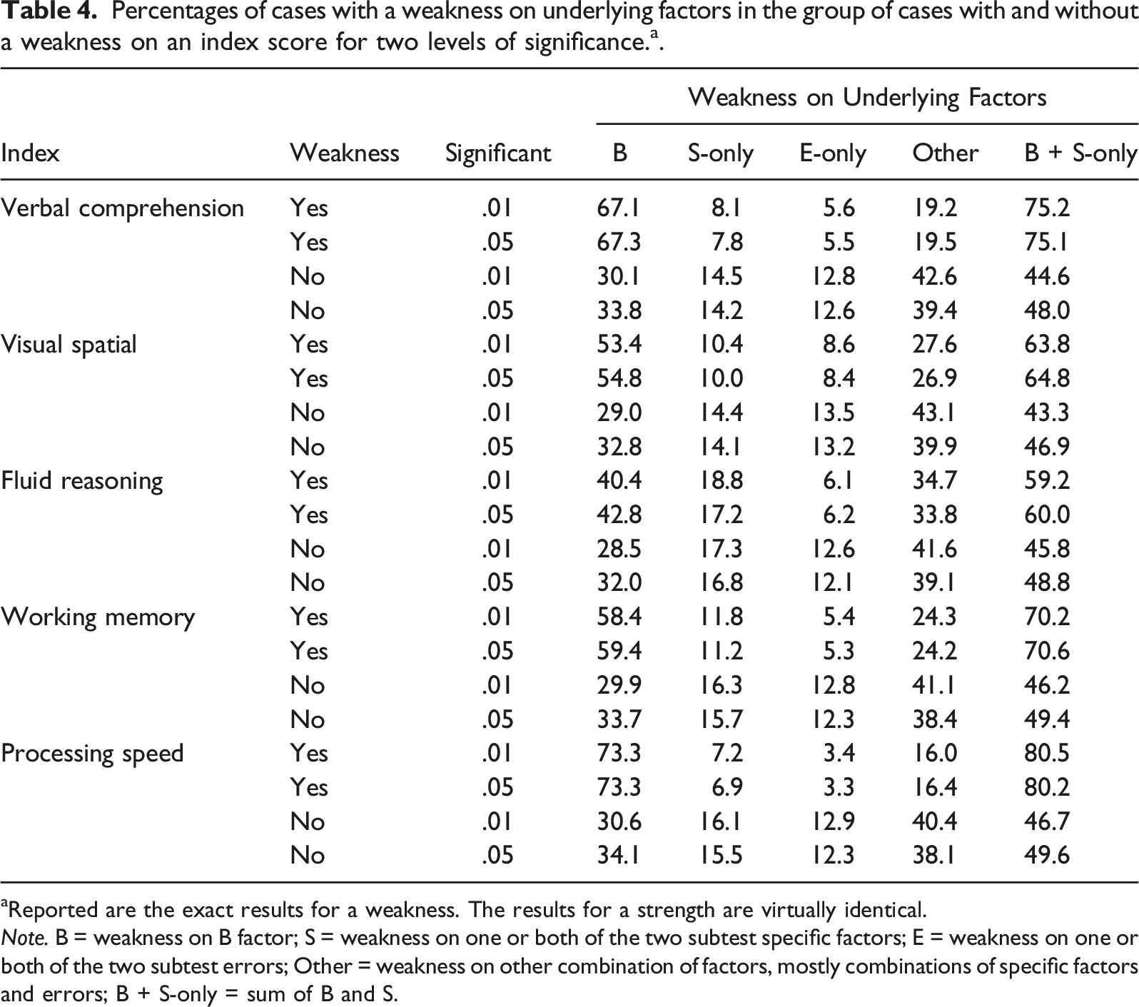
aReported are the exact results for a weakness. The results for a strength are virtually identical.
Note. B = weakness on B factor; S = weakness on one or both of the two subtest specific factors; E = weakness on one or both of the two subtest errors; Other = weakness on other combination of factors, mostly combinations of specific factors and errors; B + S-only = sum of B and S.
Several of the results in Table 4 are noteworthy. First, the results are hardly affected by the level of significance used to determine a discrepancy. Second, a discrepancy on an index score reflected a discrepancy on the underlying broad factor in 40%–74% of the cases. For Fluid Reasoning, a discrepancy on the observed index score was not accompanied by a weakness on the underlying broad factor in approximately 60% of the cases. Verbal Comprehension and Working Memory fared somewhat better. Still, for one in three cases, the discrepancy between the index and the GIS-score could not be attributed to the broad factor. Third, in 8%–20% of the cases a discrepancy was solely due to subtest specific factors. Finally, turning to cases without a discrepant index score, it appeared that approximately 30% of these cases (about one in three) did nevertheless have a discrepancy on the underlying broad factor. The results show that a discrepancy on the underlying broad factor was about 1.3 to 2.4 times more likely in cases with than in cases without a discrepant index score. The average likelihood was 1.88. According to Chen et al. (2010), these likelihoods mostly indicate a small effect. When taking a lenient approach by adding discrepancies on the broad and subtest specific factors (last column of Table 4), the average likelihood even decreased to 1.5.
Discussion
The clinical use of profiles has been hotly debated within the domain of intelligence testing (McGill et al., 2018; Watkins & Canivez, 2022), as well as outside this domain, for example for the diagnosis of learning disabilities (Fletcher & Miciak, 2017). Many studies have been conducted that question the reliability and validity of patterns of strengths and weaknesses (Canivez et al., 2017; Macmann & Barnett, 1997; Miciak et al., 2018; Watkins et al., 2022). The current study examined the validity of a profile of strengths and weaknesses for the Dutch WISC-V. The results replicate and extend previous findings on the validity of WISC-V profiles.
As in studies on the US version of the WISC-V (e.g., McGill et al., 2018), most of the variance in the subtest and index scores of the Dutch WISC-V was accounted for by the g factor. The broad factors that indexes, and the associated subtest scores, are assumed to reflect, explained little variance in these scores. Especially the subtest and index scores for Fluid Reasoning, Visual Spatial and Working Memory were hardly determined by their broad factor. As an extension to previous studies, a distinction was made between subtest specific variance and error variance, for the Dutch as well as the US version of the WISC-V. The results showed that, in both the Dutch and US versions, for the majority of the subtest scores, and about two out of five index scores, task specific factors accounted for more variance than the broad factor. In all, as in earlier studies (e.g., McGill, et al., 2018), the subtest and index scores of the WISC-V hardly seem a reflection of the broad factors, after the g factor is removed.
On the basis of similar findings, Canivez and colleagues (e.g., Canivez et al., 2017; Dombrowski et al., 2018; Watkins & Canivez, 2022) have repeatedly concluded that index scores are not sufficiently valid to be used for clinical purposes. Although this conclusion might be warranted, it does not seem to follow directly from the lack of broad factor variance reflected by the index scores. First, the crucial assumption of Canivez and colleagues is that the validity of an index score should be assessed after g factor variance has been deleted. In contrast, it could be argued that the heavy involvement of the g factor in the various subtest and index scores might not be a problem for their interpretation. For example, a vocabulary test is arguably the best reflection of vocabulary knowledge, despite the fact that the test score might be substantially related to g. The two subtests constituting the Working Memory index clearly encompass the domain of working memory. Moreover, in some taxonomies of cognitive abilities, g is not even involved (Canivez & Youngstrom, 2019) or an emergent property of a dynamic system of reciprocal interactions among cognitive abilities, as in the mutualism theory (van der Maas et al., 2006; 2019). According to these theories, there would be no reason to partial out the g factor variance that index scores have in common. Second, as argued in the Introduction, the main issue concerns the interpretation of index difference scores as these form the basis of profiles of strengths and weaknesses. The g factor is hardly involved in these scores. In all, it might be debated that the substantial amount of g factor variance in the index scores hampers their interpretation.
Irrespective of the taxonomy or theory of cognitive abilities, the heavy involvement of the g factor in the index scores does become a problem when profiles of strengths and weaknesses are considered based on index differences scores. The current results show that, as in the index scores, the broad factors accounted for relatively little variance in these scores. For Fluid Reasoning, this was even less than 10%. However, unlike the index scores, the major problem with the index difference scores is that the remaining variance is hard to interpret. Depending on the particular index difference score, between 50% and 91.5% of the variance was due to a mixture of subtest specific factors and errors, as well as broad factors deemed to be irrelevant for the particular index (see Table 3). As a result, these difference scores contain insufficient systematic true score variance. Thereby, these scores are of little use for clinical interpretation.
Taking a more lenient approach, one might argue that also subtest specific factors should be taken into account to judge the validity of a difference index. In this approach, the index score is not merely conceived as the reflection of the common variance of the subtests but reflects the level of performance in a particular domain. Even taking this lenient approach, however, several difference index scores, especially the Fluid Reasoning and Visual Spatial difference indexes, hardly capture the minimally required amount of variance, and none account for the preferred amount to warrant a valid clinical interpretation (Reise et al., 2013). Moreover, though some subtest specific factors might have a substantive interpretation, such as for Digit and Picture Span, for most subtest specific factors the theoretical interpretation is largely unknown
The consequence of a lack of validity of index difference scores was further examined by considering the extent to which a significant discrepancy on an index (strength or weakness) could be attributed to an accompanying discrepancy on the underlying broad and test specific factors. The criteria for a discrepancy were taken from the Dutch manual of the WISC-V (Wechsler, 2018), making the results directly relevant for clinicians. The results provide further insight in what it means when difference index scores are insufficiently determined by the broad factors. Especially, the Fluid Reasoning difference index hardly reflected the broad factor. As a result, in the simulated data a discrepancy on this index was accompanied by a discrepancy on the underlying broad factor in only 40% of the cases. Similarly, only 50% of the cases with a discrepancy on the Visual-Spatial index appeared to have an underlying discrepancy on this broad factor. Discrepancies on the other indexes fared a little better. But overall, about one in two to one in four cases with a discrepancy on an index did not have an accompanying discrepancy on the underlying broad factor. These results were hardly affected by the level of significance used to determine a discrepancy. A higher significance level did result in a lower percentage of cases with a discrepancy, but did not further ensure that a discrepancy was accompanied by a discrepancy on the underlying broad factor.
Finally, a comparison was made between cases with and without a discrepancy on a particular index. Given the somewhat arbitrary cut-off to determine a discrepancy, it was to be expected that a substantial number of cases without a discrepancy on an index, did nevertheless have a discrepancy on the underlying broad factor. A weakness on an index only increased the likelihood of an underlying discrepancy on the broad factor by a factor 1.5 to 2. Such a small effect is in line with the finding that many leaning problems have multiple probabilistic causes (Pennington, 2006; van Bergen et al., 2014). However, with respect to the implications of strengths and/or weaknesses in an IQ profile for a specific learning disorder, two likelihoods are actually at stake. One is the likelihood of a learning disorder given a weakness on a certain index, and the second is the likelihood that the weakness is related to poor performance on the broad factor. When both likelihoods are rather small, it becomes difficult to tie a learning problem of a particular person to a weakness on a broad factor.
Limitations
All results of the current study are based on the Dutch factor model of the WISC-V with five first order factors (Wechsler, 2018). In this model, similar to the US model (Dombrowski et al., 2015, 2017), the first order factors Visual Spatial and Fluid Reasoning seem hard to distinguish (see Figure 1). It might be regarded a limitation that the current study was not based on the proper factor model, probably the four factor model in which the Visual Spatial and Fluid Reasoning tests form one factor. However, the five factor model currently forms the basis of the index scores used by clinicians. Moreover, as the results show, the redundancy of the five factor model is largely responsible for the little variance that can be attributed to the broad factor in the Visual Spatial and Fluid Reasoning index and difference index scores. The choice for a four factor model might not be a much better solution. The more general point is that index difference scores reflect little variance of the broad factors if the first order factors in the factor model are strongly correlated with the second order g factor. In a four factor solution the correlations among the factors are also (too) high (Canivez et al., 2017).
A further limitation of the use of the Dutch factor model of the WISC-V could be that the results, especially of the simulation study, might not generalize to versions of the WISC-V used in other countries. However, the factor models of the various versions tend to be highly similar (e.g., Canivez et al., 2017; Lecerf & Canivez, 2018; Pauls & Daseking, 2021). Moreover, the current study showed that the sources of variance in the subtest and index scores of the Dutch and US version are highly similar as well. As the results on the index scores directly translate into the index differences scores, it seems highly likely that a simulation study based on the US factor model of the WISC-V will give similar results and leads to the same conclusions.
The Use of Profiles of Strengths and Weaknesses
The current study, as with previous studies, strongly suggests that patterns of strengths and weaknesses lack sufficient validity for clinical use. Nevertheless, clinicians continue to use the WISC profiles. In closing, a number of reasons are considered that might be responsible for this continuing use in clinical practice. One reason is that particular profiles have often been observed in groups of individuals with specific disorders (van Iterson et al., 2015; Toffalini et al., 2017). Possibly, clinicians might not realize that profiles observed at the group level are often not representative for substantial numbers of individuals belonging to such a group. Another reason is probably that the use of profiles is still taught to students who will eventually enter clinical practice (Farmer et al., 2021). A final reason could be that strengths and weaknesses on the WISC-V are automatically provided by the publisher to the users who are, subsequently, tempted to interpret them. As a result, the use of profiles often concerns post hoc interpretations, whereas as a proper diagnostic process should start with hypotheses to explain the problem at hand. Such hypotheses could involve a weakness or strength across the various indexes of IQ, although in many instances an absolute strength or weakness might be more important than a relative. But even in the case of an hypothesis about a discrepancy, which is important and can be posed before an IQ test battery is administered, it seems doubtful that the hypothesis can be properly tested given the lack of validity of the scores that are available to signal strengths and weaknesses.
Footnotes
Acknowledgments
I would like to thank Kees-Jan Kan for generating the data, Lauren McGrath for providing me with the reliabilities of the subtests of the US version of the WISC-V and Madelon van den Boer for her comments on an earlier version of this paper
Declaration of conflicting interests
The author(s) declared no potential conflicts of interest with respect to the research, authorship, and/or publication of this article.
Funding
The author(s) received no financial support for the research, authorship, and/or publication of this article.
Appendix A
Omega hierarchical scale, ωh, denotes the proportion of variance that can be accounted for by the broad factor in the index score. According to Brunner et al. (2012, p. 825), ωh can be defined as
where λij denotes the standardized factor loading of subtest Yi on factor j and ei the standardized variance of the unique factor related to subtest Yi. J is the index for the factors involved in an index (the g-factor and the broad factor) and p indicates the particular subtests, here two. When ei is split in task specific variance, si, and error, εi, ωh becomes
Omega hierarchical scale for the proportion of variance accounted for by the subtest specific variance can be defined as
Omega hierarchical scale for the proportion of variance accounted for by the subtest error variance can be defined as
Appendix B
# In order to generate multivariate normal data, load package MASS
library(MASS)
# in order to be able to replicate the outcome, choose a random seed
set.seed(2021).
## Setup
n <- 1000000 # number of individuals
ng <- 1 # number of general factors
nf <- 5 # number of group factors
nu <- 10 # number of specific (unique) factors
ne <- 10 # number of error terms
nv <- ng + nf + nu + ne # total number of (latent) variables
# generate values for the nv variables
# means are set to 0 for all variables
# sds to 1
# assume variables are all independent (diagonal variance-covariance matrix)
# empirical = TRUE means generate population data/‘exact simulation’.
Data <- mvrnorm( n, rep( 0, nv ), diag( nv ), empirical = TRUE ).
# add column names to the dataset.
colnames( data) <- c( 'g', paste0( 'f', 1:nf ), paste0( 'u', 1:nu), paste0( 'e', 1:ne ))