
Abstract
This study develops a cost model covering monetary and environmental damage costs for source-separated biowaste collection. The model provides an improved basis for decision-making by including environmental damage costs compared to the assessment that considers the only monetary cost. The monetary cost calculation integrated route optimisation using existing road networks, while the environmental damage cost was estimated using the life cycle impact assessment method based on the endpoint (LIME) model. The model was tested in the Finnish case where the new law implements the stricter requirement for source-separated biowaste. The costs of collection, transportation and treatment of three different scenarios were assessed: mixed waste under the old law (MW-OL), biowaste under the new law (B-NL) and mixed waste without biowaste under the new law (MW-NL). The results showed the economic and environmental benefits of sourced separated biowaste. The overall cost of collection and transportation (CT) under the old law and new laws were 80.7 € Mg−1 and 81.1 € Mg−1, respectively. Treatment costs were 79 € Mg−1 and 64.8 € Mg−1 under the old and new laws, respectively. The damage costs for CT under the old and new laws were 0.23 € Mg−1 and 0.24 € Mg−1, respectively. At the same time, the damage costs from the treatment stage were 4.9 € Mg−1 and 3.5 € Mg−1 under the old law and new law, respectively. The model supports decision-making when the collection scheme requires a change. Failing to plan an optimised solution and cost will lead to inefficient systems.
Introduction
Waste generation is an unavoidable consequence of anthropogenic activities that may damage human health and the environment (Logan and Visvanathan, 2019). Consumption patterns, population growth, income and climate affect the quantity and composition of municipal solid waste (MSW) generation (Kinobe et al., 2015; Ragossnig and Schneider, 2019). Consequently, MSW varies among regions, while at the same time, it becomes crucial to manage MSW properly to protect human health and the environment. With the new paradigm of the circular economy (CE), waste is seen as a resource, so the end-of-life (EoL) notion should be phased out by recovering the remaining value of the waste (Geissdoerfer et al., 2017).
Policies are the key driver to achieve circular waste management in Europe (Wilts et al., 2016). European Commission formulates directives that should be achieved by the members without specifying the laws or means to fulfil the target. An example is the waste directive framework that requires the country members to recycle biowaste up to 70% by 2030 (European Commission, 2021). This affects how waste management policy is applied in each country member. In Estonia, the biowaste collection is a source-separated for at least 10 apartments (Tallinn, 2022). Sweden has a different approach where the target is set on the national level, guiding the municipalities in structuring the waste collection and treatment. Household biowaste can be collected separately or as a fraction of mixed waste, with about two-thirds of all municipalities collecting source-separated food waste at varying degrees (Avfall Sverige, 2018). Denmark applies a similar approach as Sweden regarding biowaste collection (State of Green, 2017). Finland amended the Waste Act (646/2011), which sets the goal for the reuse and recycling of 55% of MSW in 2025, 60% in 2030 and 65% in 2035. The new legislation also tightens the obligation of biowaste collection. Biowaste should be collected separately if the residential property has at least five apartments which is stricter than 10 apartments in the previous legislation. Source-separated municipal waste effectively optimises resource recovery and avoids landfilling as long as proper infrastructures are available (Daskal et al., 2018; Kawai and Huong, 2017). A source separation system is generally more complex and costly than a mixed waste system, and it involves more stakeholders and alternatives for collection routes (Lavee and Nardiya, 2013). It also requires higher collection costs, more labour, new infrastructure and vehicles (Groot et al., 2014). Therefore, estimating the economic implication of implementing a source-separated collection system is imperative to formulate a charging method to cover the entire cost. It is especially significant since the collection and transportation (CT) stage may contribute up to 70% of the total cost of waste management (Rathore and Sarmah, 2019).
Previous studies about waste CT focused mainly on investigating the shortest distance and fuel consumption (e.g. Edwards et al, 2016; Kinobe et al., 2015; Nguyen and Wilson, 2010) as well as the monetary costs incurred (e.g. Boskovic et al., 2016; Larsen et al., 2010). Meanwhile, the environmental damage cost in waste CT is still underrepresented. Therefore, more accurate analysis employing real road networks to optimise collection routes as well as estimate monetary costs and damage cost is important.
This research aims to develop a monetary and environmental damage cost calculation model for waste CT. The calculation of monetary cost and environmental damage cost can provide a more comprehensive insight into which trade-offs may occur. We also utilised a tool that allowed the use of an actual road network. The applicability of the cost model is demonstrated through a real case study of Kauhajoki municipality in Finland. The amended Waste Act (646/2011) resulting in new legislation that requires biowaste separation for residential property with at least five apartments, compared with 10 apartments in the previous legislation. The amended legislation creates new clusters of properties that necessitate a separate organic waste collection; hence, new route planning is needed. Specific objectives are then formulated to achieve the aim of the study by focusing on: (i) optimisation of the waste collection route, (ii) identification of the monetary and environmental damage cost (€ Mg−1-waste) for CT, (iii) comparison of the monetary and damage cost of biowaste treatment in waste-to-energy (WtE) and anaerobic digestion (AD) facility and (iv) investigation of sensitive parameters in the cost model. The research can denote how to deal with the challenge of transitioning toward CE, where a source-separated system will be the norm.
Materials and methods
Study area
The study area comprises Kauhajoki municipality in the Southern Ostrobothnia region of Finland, which covers the area of 1315 km2 with 13,172 inhabitants (Kauhajoki, 2020). The temperature varies from −11 °C up to 21 °C throughout the years. The warm season lasts for about 3 months from June to August with an average temperature of 16 °C, whereas the cold season lasts for almost 4 months, from December to March, with an average temperature below 1 °C (Weather Spark, 2021). The growing session starts at the end of April and lasts for about 140–175 days in the area of study (Finnish Meteorological Institute, 2020).
The publicly owned waste management company provided data concerning the study area where the law will affect the collection scheme. The data included the location of collection points (CPs) and the total number of households being served. The number of CPs is 198, and it comprises 2202 individual households. The collected waste is transferred to the transfer station (TS) in Teuva, a nearby municipality, and gathered collectively with waste from neighbouring areas. The waste is then transported to the treatment facility in Vaasa region for about 82 km from the TS where WtE and AD are situated at the same area. Figure 1 displays the location of the CPs, garage (G), TS and AD.
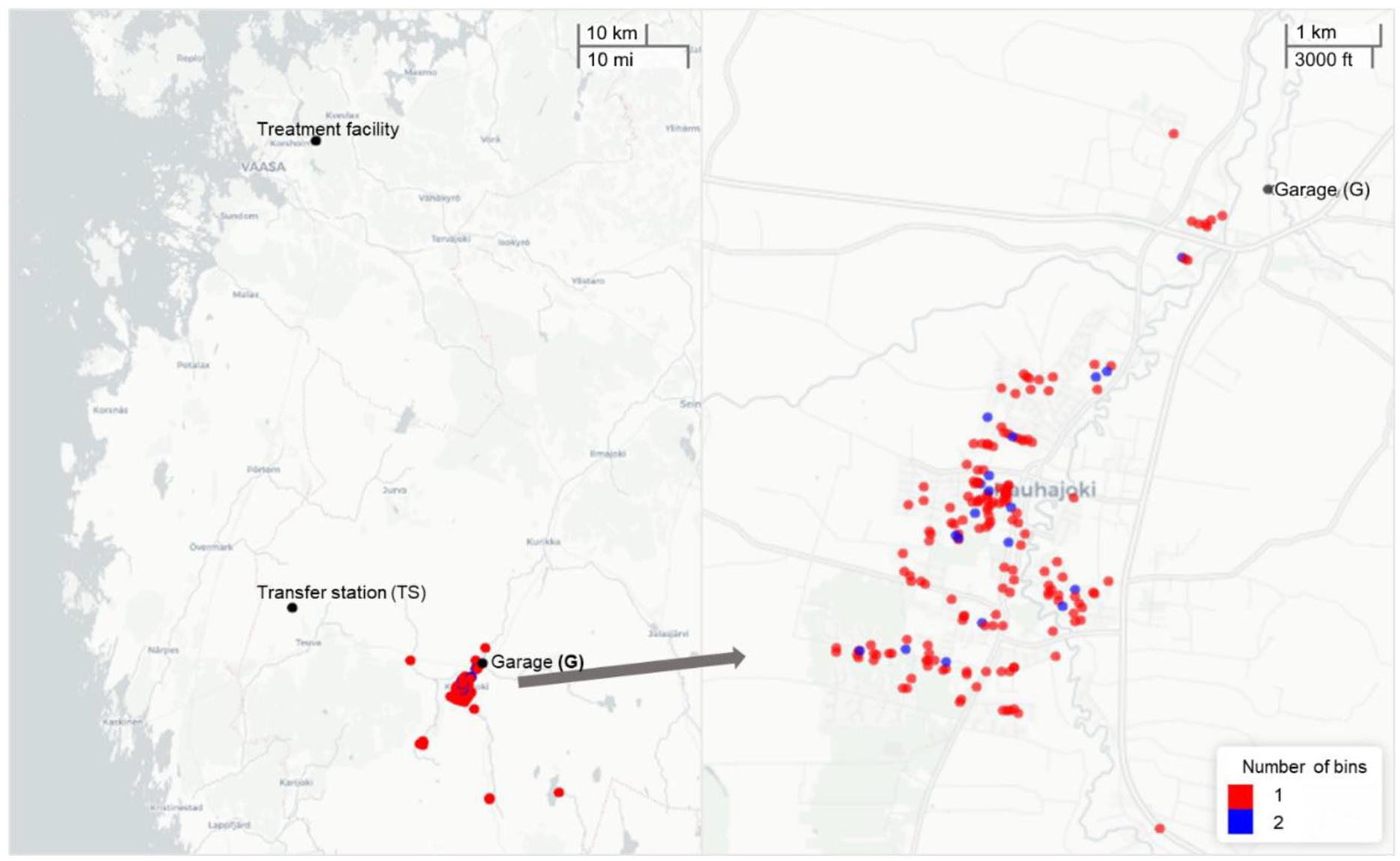
Left: Location of the collection points, garage, transfer station and anaerobic digestion. Right: The concentrated CPs.
Some of the CPs are scattered and located near the bounding coordinates. However, most CPs are concentrated in the built-in area (Figure 1). Each CP has a different number of waste bins (wheelie bin) with a total volume of 240 L. One bin is used for 5–19 households, whereas two bins cover 20–45 households.
The amended waste act commits to improving collection and recycling by increasing new targets for waste separation and recycling. The previous waste act required source-separated biowaste for a minimum of 10 dwellings clustering together. With the amended version, a municipality must collect biowaste separately from residential properties with minimum dwellings of five no later than May 2024 (Botniarosk, 2020). Containers to separate waste, including mixed waste (for incineration), biowaste, paper, metal packaging, glass packaging, cardboard packaging and plastic packaging, are provided in the residential properties with at least 10 dwellings. For the dwellings of 5–9, it is compulsory to provide containers for mixed waste and biowaste, whereas the other types of containers are optional. Lastly, for dwellings between 1 and 4, biowaste separation is not required, and it can be collected together in the mixed waste container. In addition to curbside containers, a bring-in scheme is also applied through ecopoints and recycling stations. There are more than 2500 ecopoints throughout Finland where the inhabitants can bring their packaging and paper waste. Recycling stations are facilities similar to ecopoints that accept a wider variety of waste, including stone material, electrical and electronic equipment, wood or hazardous waste.
The new policy will create a cluster where biowaste should be collected separately. The old policy collects mixed waste once a week. Whereas the new one collects biowaste weekly during summer (12 weeks) and fortnightly for the rest of the year (40 weeks). The remaining mixed waste is also collected in a fortnightly manner throughout the year. The collection starts with the vehicle leaving the G, driving to dwellings, and collecting the waste. After completing the collection, the vehicle goes to the TS, where the waste collected from Kauhajoki is combined with waste collected from neighbouring areas. A bigger vehicle then collectively transports the waste to the treatment facility area, where AD and incineration are located within the vicinity area. In this study, different terms are used to describe the activities of transporting waste. Collection refers to the activity where the waste in each CP is picked up, whereas waste transportation concerns transporting waste from TS to the final treatment facility AD.
The scenario covered by this study includes mixed waste under the old law (MW-OL), biowaste under the new law (B-NL) and mixed waste without biowaste under the new law (MW-NL). These three scenarios applied different collection frequencies where MW-OL (16 Mg truck) and MW-NL (20 Mg truck) collect the waste weekly and fortnightly throughout the year, respectively. Meanwhile, B-NL collects the waste weekly during the summer period (8 Mg truck) and fortnightly for the remainder of the year (16 Mg truck). The waste generation was estimated at around 6.6 kg household−1 week−1 (MW-OL), 2.6 kg household−1 week−1 (B-NL), and 4 kg household−1 week−1 (MW-NL) (Botniarosk, 2020; HSY, 2021).
Route optimisation
Waste CT can be seen as a conventional vehicle routing problem with a few caveats, such as the limited capacity of the vehicle and different quantities of waste in each CP (Nambiar and Idicula, 2014). In this study, there were two routes of optimisation for waste CT: (i) waste collection where the vehicle (vehicle 1) leaves the G, collects the waste, drives to TS and goes back to the G, (ii) waste transportation where the vehicle (vehicle 2) transports waste from the TS to the treatment facility such as WtE or AD plant and drives back to the TS. Vehicle 2 has a bigger capacity since it transports waste gathered from multiple collection areas. The sequence of waste CT are presented in Figure 2.
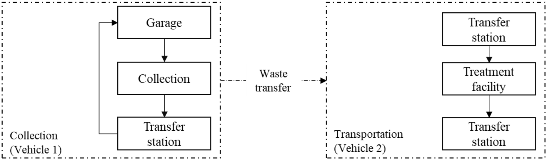
The sequence of waste CT.
Route optimisation was executed using Open Door Logistics (ODL) software. ODL is a geographic information system (GIS) software built on Graphhopper and Jsprit library, whereby the optimisation uses real road networks (Welch, 2017). The user inputs information such as service time, waste quantity in each CP, the geocode of CP, time constraint and capacity constraint. It will generate the optimal route, including travel time, distance and waste quantity in each road segment.
Cost calculation
The costs consist of monetary costs and damage costs. Monetary costs were vehicle cost, bin cost, fuel cost, labour cost and treatment cost. Damage cost indicates the monetary value of welfare losses due to the impacts of emissions caused by anthropogenic activity on the environment (Liu et al., 2021). In this case, the emission is caused by collection, transportation and treatment. Usage rate was applied to the annualised fixed cost of truck and bin so that the cost incurred is associated with the use of the infrastructure. The results are expressed as € Mg−1-biowaste as well as the annual sum cost in €. The analysis was conducted to estimate the total cost before and after the new law is applied, hence the implication of the new law could be inferred by comparing these two types of costs.
Vehicle cost
The vehicle cost refers to the fixed annual capital costs, insurance, maintenance, licence, oil and miscellaneous costs (COWI, 2004). Capital cost is a one-time expense incurred due to the purchase of the vehicle and allocated equally throughout the vehicle’s lifetime. Other cost components were estimated using a percentage of the capital cost (detail is provided in the Supplemental Table 1).
To calculate annualised capital cost (A), equation (1) was applied:
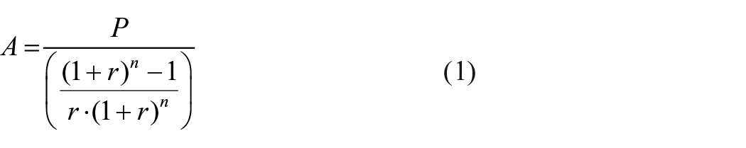
where P,
where
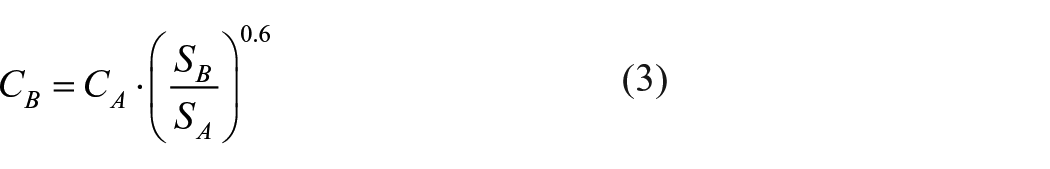
Price adjustment was also required when the available information showed a different truck capacity than the desired one. The calculation to approximate capital cost for different capacities follows the rule of six-tenths, as shown by equation (3) (Serna, 2018):
where

where

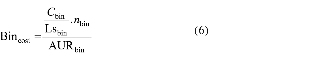
Bin cost
Bin cost was calculated based on the annualised investment divided by the usage rate. The cost estimation concerning bin cost per Mg biowaste was calculated using equation (6). The price of a single bin (€), the lifetime of a bin (year), the number of bins and the annual usage rate (Mg year−1) are represented by
Fuel cost
The cost of fuel consumption was the sum of service consumption and travel consumption then divided by waste quantity (
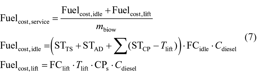
Fuel consumption from travelling
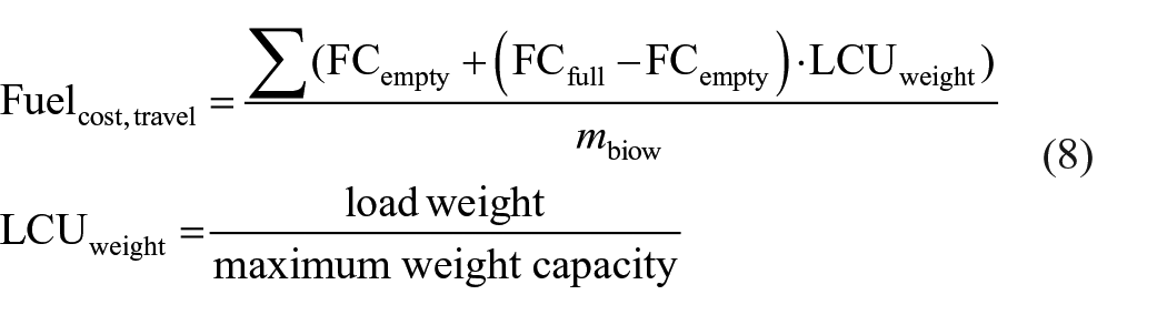
where
Labour cost
Labour cost refers to the wage of the driver and bin loader for waste collection, whereas waste transportation requires only a driver. The labour cost was about 25 € hour−1 (see Supplemental Table 1). Equation (9) is used to calculate the labour cost.

where
Treatment cost
Information regarding treatment costs in WtE and AD were calculated using tools that were developed for WtE optimisation (Mayanti et al., 2021b) and marginal cost estimation of an AD (Mayanti and Helo, 2021). The calculation for WtE was modified based on the waste composition in this study (Supplemental Table 2), whereas the AD in this study was assumed to treat kitchen waste. The lower heating value (LHV) and life cycle inventory (LCI) of waste treated in WtE were estimated by a tool called waste incineration life cycle inventory tool (WILCI) (Beylot et al., 2017). The methane potential, which determined the total methane production and its fugitive, was estimated using stoichiometry based on waste chemical composition (Supplemental Table 1). The focus of the study was on the CT since they will be affected directly by the new law. However, including the treatment stage could provide more comprehensive knowledge of whether a trade-off exists between treatment schemes.
Damage cost
Damage cost was calculated for CT as well as the treatment phase. The method to calculate damage cost was the Life Cycle Impact Assessment Method based on Endpoint 3 (LIME3) model (Inaba and Itsubo, 2018; Liu et al., 2021). The model was initially established by Japan’s Ministry of Economy, Trade and Industry to portray the environmental and social situation in Japan (Itsubo and Inaba, 2003). It has been undergoing development, and in 2016 LIME 3 model was developed with various coefficients applicable to different countries (Inaba and Itsubo, 2018). Applying LIME to obtain environmental damage costs starts with building inventories, followed by multiplying the inventories with the factor/coefficient. The framework used to calculate damage cost in waste treatment is shown by Figure 3 (Liu et al., 2021). Three coefficients can be used to obtain different results, namely damage factor (DF), weighting factor (WF) and integration factor (IF). The last coefficient is a product of multiplying DF with WF. The environmental damage costs can be obtained by multiplying emissions in the inventory with the IF.
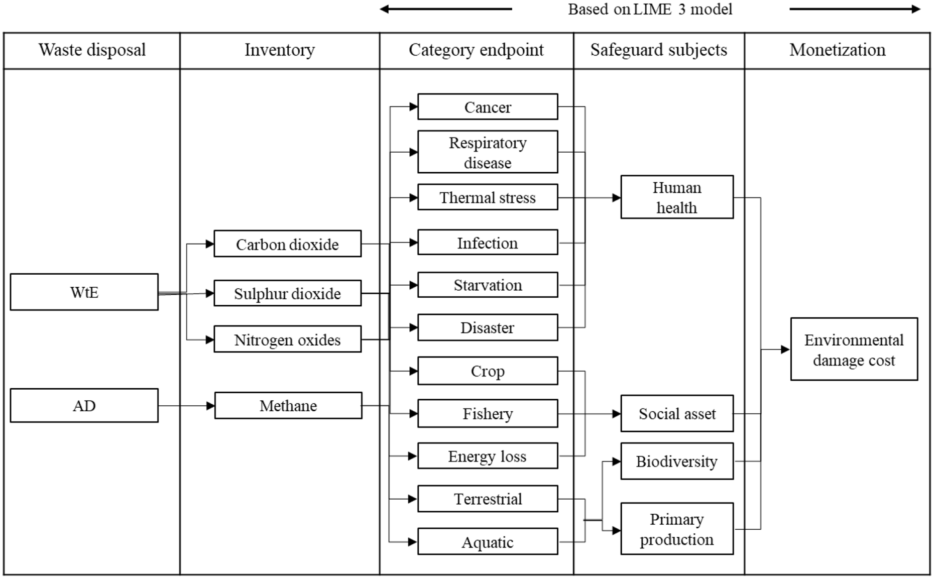
Framework of environmental damage cost of WtE and AD.
Emission inventory
Emission inventories were collected from the collection, transportation, and treatment phase. The emission from the CT phase included CO2, and it was calculated using the emission factor (EF) issued by the Finnish Standards Association (2013), as shown by equation (10).

For the treatment phase, CO2 was not considered. It is assumed that CO2 from the biowaste during treatment is equal to CO2 absorbed during biomass production; therefore, it should not be reported (IPCC, 2019). Sulphur dioxide (SO2), nitrogen oxides (NOx) and non-methane volatile organic compounds (NMVOC) were considered for damage cost estimation. Other emissions were not included due to the limited coefficient in the LIME database. Moreover, other emissions can be considered marginal (Liu et al., 2021). The emission inventories from the incineration process were obtained using the WILCI (Beylot et al., 2017). Meanwhile, methane (CH4) was the emission considered from AD due to unintentional leaks, accounting for 1% of total CH4 production (Liu et al., 2021). The general emission equation from AD was calculated using equation (11).

where
Damage cost calculation
After collecting emission inventories, the damage cost calculation can be estimated using the LIME database (LCA Society of Japan, 2018). The general equation to estimate the environmental damage cost is shown by equation (12).

where
Sensitivity analysis
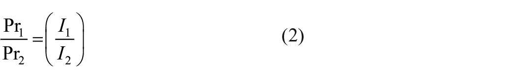
Sensitivity analysis examines the results as an effect of modifying the inputs. Perturbation analysis was applied by changing the input parameters by 10% one-at-a-time while maintaining all other parameters the same as the baseline values. The outputs from perturbation analysis were then used to calculate the sensitivity ratio (SR), as shown in equation (13). SR is the ratio between two relative changes, namely the relative change of result and input parameter (Bisinella et al., 2016).
Results
Route optimisation
Route optimisation was done for CT. The same routing was obtained for MW-OL, B-NL, and MW-NL. The total waste generated ranged from 5.7 Mg up to 17.6 Mg in each collection. During the collection stage, different results are displayed by different scenarios. The travel time and service time required for MW-OL and MW-NL were 4.12 and 4.51 hours, respectively. The B-NL scenario needed 4.12 hours of travel and 3.71 hours of service. In between CPs, the velocity varied in each road segment, showing the minimum and maximum values of 30 km h−1 and 59.5 km h−1, respectively. Total fuel consumption for MW-OL and MW-NL was not much different, as shown by 64.5 L and 65.9 L in each collection, respectively. For B-NL, fuel consumption during summer collection would consume 57 L, and the rest of the year would require 59.7 L. The Supplemental (Figures 1 and 2) presents the CT route results.
Route optimisation for waste transportation was simple since it only had one stop in the treatment facility. The transportation used a truck with a 32-Mg capacity, transporting waste gathered from multiple locations. The travel and service time required to complete the transportation was about 2.26 h and 0.75 h, respectively, with a total distance around 165 km. Table 1 displays the summary results of route optimisation for both CT.
Summary of route optimisation of waste CT.
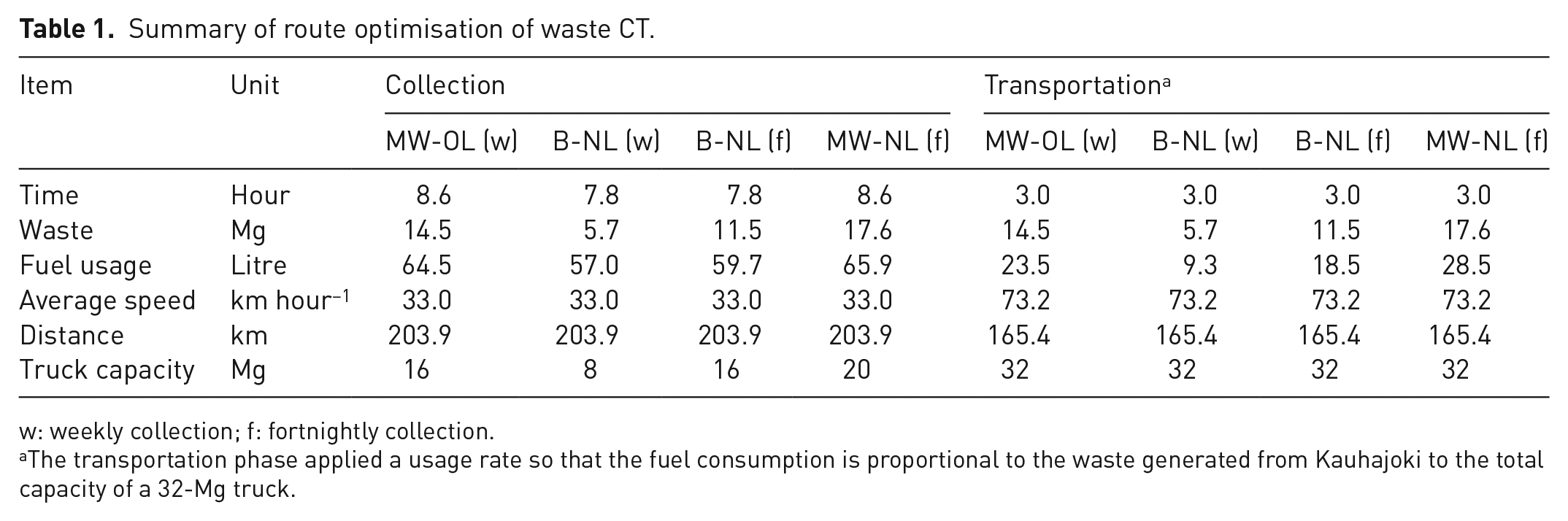
w: weekly collection; f: fortnightly collection.
The transportation phase applied a usage rate so that the fuel consumption is proportional to the waste generated from Kauhajoki to the total capacity of a 32-Mg truck.
Monetary and damage costs of CT
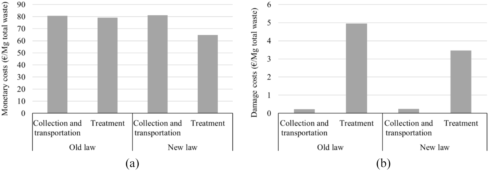
The monetary and damage costs results will be presented as absolute annual value and relative cost per Mg waste. The assessment resulted from CT costs for about 80.7 € Mg−1 total waste under the MW-OL scenario. Under the new law, B-NL and MW-NL would cost 91 € Mg−1 and 74.7 € Mg−1, respectively. On an annual basis, the cost under the new law will be equal to 81.1 € Mg−1 of total waste. Figure 4 shows the annual cost items for waste CT under the old and new laws.
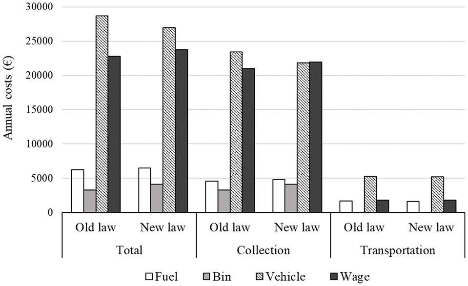
Annual monetary costs of waste CT.
A similar pattern was observed in the old law and new law scenarios where the highest contributor to the total cost was vehicle costs ranging between 44 and 47%, followed by wage contribution for about 37–39%. Contribution from bin and fuel consumption was relatively low and did not exceed 16%. The analysis showed that separating biowaste caused a slight increase of about 359 € annually, translating into 0.5 € Mg−1 total waste.
The results of damage costs under the new law showed a marginal increase compared to the old law, corresponding to the monetary costs results contributed by the fuel consumption. The annual damage costs difference between old and new laws was about 9.1 €. The damage costs of the old law and new law that resulted from CT were 0.23 € Mg−1 and 0.24 € Mg−1, respectively. Figure 5 shows annual damage costs under the old and new laws for waste CT.
Annual damage costs of waste CT.
Monetary and damage costs of waste treatment
Cost calculation of waste treatment was applied using the system expansion principle. The products generated from waste treatment were deemed as credits for being an alternative in substituting the original products (e.g. biosolids could substitute artificial fertiliser). It brought revenue in the monetary cost calculation; meanwhile, it was considered environmental credits instead of damage in the damage cost calculation. Before the new law takes effect, mixed waste is treated in WtE. The new law will treat the biowaste in AD and the remaining mixed waste in WtE. The treatment cost using WtE associated with MW-OL was 79 € Mg−1 total waste. Under the new law, the cost was around 64.8 € Mg−1 total waste. It consisted of B-NL treatment using AD and MW-NL treatment using WtE, which each of them costed for about 23.3 € Mg−1 biowaste and 91.7 € Mg−1 mixed waste, respectively.
Under the old and new laws, the environmental damage costs were 4.9 € Mg−1 total waste and 3.5 € Mg−1 total waste, respectively. The total damage costs under the new law consist of treatment costs using WtE and AD for about 6.5 € Mg−1 mixed waste and −3 € Mg−1 biowaste, respectively. The damage cost due to incineration was more expensive under the new law; nevertheless AD showed negative damage cost resulting in more benefit compared with the old law. Figure 6 shows annual monetary and damage costs of waste treatment under the old and new laws.
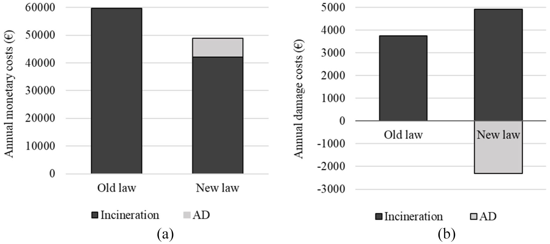
Annual monetary costs (a) and damage costs (b) under different laws.
Comparison between the old law and new law
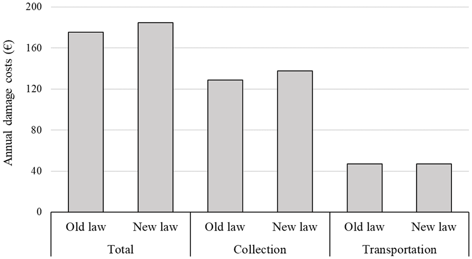
This study emphasised the monetary cost and damage cost implications of a waste diversion strategy where source-separated biowaste is implemented. Due to the new law, this diversion strategy required a new collection infrastructure that was translated into additional cost. A cost comparison between the old and the new laws was conducted to obtain a more comprehensive perspective. The old law scenario is the baseline case before implementing the source-separated biowaste strategy. It will collect mixed waste (burnable and biowaste) from the household and treat it in incineration. With the diversion strategy, biowaste is collected separately and is treated in AD. In general, the results suggested that implementing the new law would benefit both from monetary and damage costs perspectives. The overall costs of collection, transportation and treatment under the old law and new law would be around 160 € Mg−1 and 146 € Mg−1, respectively. The same pattern was found in the damage costs assessment, where the old and new law results were 5.2 € Mg−1 and 3.7 € Mg−1, respectively. Figure 7 displays the costs comparison between the implementation of the old and new laws.
Monetary costs (a) and damage costs (b) per Mg waste under different laws.
Sensitivity analysis
The SR was calculated to measure the most sensitive parameters for monetary and damage costs. If a change of parameter results in an SR value of 2.5, it indicates that a 10% increase of the parameter will increase the results by 25%. The tested parameters differed between monetary and damage costs because some parameters only affected monetary costs, such as bin price, discount rate, etc. Overall, there were 12 separate sensitivity analyses. These comprised the sensitivity analysis for the monetary cost of collection and treatment as well as damage cost for collection and treatment applied to MW-OL, B-NL and MW-NW. The complete results can be found in Supplemental Figures 3 and 4.
The SR of monetary costs applied to CT showed certain similarities. In all three scenarios, the most sensitive parameters to cost decrease were an increase in truck operating hours and lifetime. Meanwhile, waste quantity and vehicle cost were most sensitive to an increase of the costs. Overall, the SR values ranged from −0.66 up to 0.7. For the treatment using WtE and AD, different parameters were tested against different treatment methods. The similarity was found in MW-OL and MW-NL, where the treatment costs using WtE were most sensitive to the change of discount period (SR −0.4) and capital cost (SR 1). For the B-NL scenario, the most sensitive parameters were methane LHV (SR −0.5) and labour cost (SR 0.85).
For the damage costs, a similar trend showed in the results of SR on the CT. The most sensitive parameters that caused a decrease and increase in the overall damage costs were waste quantity and fuel consumption rate, respectively. The SR itself ranged for about −0.6 to 1. The most sensitive parameters for WtE treatment for both MW-OL and MW-NL were similar. The damage cost decrease was most sensitive to an increase of net efficiency of the WtE (SR −0.4 up to −0.3), whereas the damage cost increase was most sensitive to an increase of the fossil (SR 1 up to 1.4). Biowaste treatment using AD showed a difference where the overall damage cost was negative. Therefore, the positive value of SR indicates more benefit (the overall damage cost will be more negative), and the negative value of SR suggests damage (the overall damage cost will be less negative). For the B-NL scenario, the most sensitive parameters were fugitive methane (SR −0.03) and methane potential in the waste (SR 0.93).
Discussion
The importance of waste composition and quantity
Municipal waste composition and generation are affected by income, climate and demography (Kinobe et al., 2015). Hence, it varies among regions while at the same time, it is a crucial component in planning for collection, transportation and treatment. It affects the infrastructure needed, collection frequency and collection route. Waste composition is associated with the monetary costs and the environmental impact, especially during the treatment process. This study indicated the effect of waste composition on the monetary and damage costs of treatment using WtE. There was an increase in the monetary and damage costs of treating mixed waste under scenarios MW-OL and MW-NL. Although the LHV of waste in the MW-NL scenario was higher due to the removal of biowaste, the cost became higher. The damage costs were higher as the fossil carbon content in each Mg of waste was increasing. The increase of fossil carbon was mainly caused by plastic waste, which contributed to about a quarter of waste composition. Incinerating plastic waste and its association with the high environmental impact was demonstrated in a previous study done by Beylot and Villeneuve (2013). Simultaneously, the overall monetary cost was also increasing under the MW-NL scenario. WtE facility has limited thermal capacity; hence the increase of waste LHV will reduce the amount of waste being treated. The result confirms the guide provided by the waste hierarchy regarding the importance of material recovery before utilising WtE for energy recovery.
The knowledge regarding waste quantity also affects the optimisation of the collection, transportation and treatment. It determines the required infrastructures such as bin size, the number of bins, truck capacity, waste storage, feed preparation and treatment facility. This study used a value of 6.6 kg total mixed waste per household per week, consisting of 2.6 kg biowaste and 4 kg mixed remaining waste. The number was adopted from the report from waste management in Kauhajoki (Botniarosk, 2020), with an additional 5% as a buffer. The quantity of waste in the report shows the overall municipal waste, including household, private sector, public sector and other similar waste. The calculation was done using the assumption that the household generated 54% of total municipal waste (HSY, 2021).
Adding buffer value in calculation can help deal with some waste generation uncertainties. Denafas et al. (2014) reported that seasonality affects MSW composition and quantity. Statistics also show that was generation can change from year to year (Botniarosk, 2020). At the same time, too much buffer can lead to overestimation, which causes inefficient and costly systems. Evaluating the system periodically can prevent inefficiency so that collection frequency, route or vehicle capacity can be adjusted. The sensitivity analysis results also displayed the importance of waste quantity as the most sensitive parameter for the waste CT cost model. Ensuring that the data regarding waste quantity is as accurate as possible will result in reliable cost estimation. For comparison, waste generation in Kauhajoki was compared to other cities. Helsinki generates a higher household than Kauhajoki, as shown by the value of 7.1 kg per household (7.5 kg with 5% buffer), whereas household biowaste was about 2.8 kg (2.9 kg with 5% buffer) (HSY, 2021). In Copenhagen, the average household generates 3.5 kg of biowaste (3.7 kg with 5% buffer) in a week (State of Green, 2017).
Assumptions used and uncertainties of the results
Uncertainties in the results are generated by the accumulation of uncertainty present in the data input, methodologies, assumptions and formulas. The input values represent the average condition; therefore, unusual events or irregularities cannot be captured. Seasonality in the waste generation or situations that result in the vehicle moving slower can generate different outcomes. Other sources of uncertainties were the assumptions used to assess treatment costs. For the WtE facility, assumptions such as the emission factor of the air pollution control unit, the efficiency, and the amount of ash generation will affect the calculation results. Meanwhile, parameters in AD including the rate of fugitive methane, methane potential, efficiency and biosolids generation, also influence the outcomes. This study utilised typical WtE and AD used by previous studies (Mayanti and Helo, 2021; Mayanti et al., 2021a), since these studies used the Finnish context in building their calculation tools. Since it is not possible to test every possible assumption, sensitivity analysis was applied to understand the effect of each parameter. The assessment was conducted by applying perturbation analysis to obtain information concerning the magnitude of change in the results regarding shifting the input value. Knowledge about the most sensitive parameter could improve decision making and help assess the risk of a particular strategy associated with a particular input value. Moreover, it assists in predicting the results of a decision if a situation turns out to be different from the baseline prediction.
The results are expressed in € Mg−1 total waste; however, the overall annual cost was also assessed to provide a more comprehensive picture regarding the implications of changing waste management policy. Different studies used different measuring units, and implementing both could be useful to compare results. Martinez-Sanchez et al. (2015) reported that the collection cost of separated biowaste in Denmark was 96.3 € Mg−1, whereas this study showed a result of 91 € Mg−1 biowaste. Seyring et al.(2015) reported the collection fee of separated biowaste in Tallin was charged between 1.5 and 4.2 € bin−1 emptying for a bin size of 240 L. The same bin size was utilised in this study, which resulted the cost of 2.4 € bin−1 emptying. In general, some results of this study correlated with others. The difference could be caused by the size of the study area, input parameters or assumptions. Comparing results can provide useful information concerning the possibility to generalise the study to another context.
Implications and limitations
The results provide information regarding the optimised route, monetary cost, and damage cost regarding new waste management regulations. It will have implications for different actors such as waste management companies owned by several neighbouring municipalities, households, property owners, waste treatment operators and the government. Monetary cost aimed to quantify the real and internal waste CT costs in order to prepare the infrastructure for the transition toward a source-separated waste system. The real cost is what the waste management company needs to be aware of in order to determine the fee that the household will bear. The environmental damage cost was applied to provide a comprehensive perspective from an environmental perspective. The overall results indicated that the new law would benefit from economic and environmental perspectives. A good planning becomes the key for all stakeholders involved in a waste management system. For example, some of the most sensitive parameters during waste collection were the waste quantity and vehicle cost. It pointed out that estimating waste generation was important since it would affect the choice of truck capacity.
For the authorities, the findings on monetary cost can be used as a reference in organising the CT operation (tender process and awarding contracts). The costs are split into two parts, where different vehicles are in charge of the CT. This separation helps clarify the cost incurred in each part, especially when the authorities plan to hire different waste transporters. This study provides preliminary knowledge for the authorities regarding the route, cost and emission. They will be able to fine-tune what the waste transporters offer to avoid an inefficient system. They can also start communication with property owners and households to inform the approximate additional waste bin and fee.
The study requires various inputs along with the choice of boundary, type of parameters and method that can lead to uncertainty. Primary data provided by waste management companies can reflect the actual situation; however, the remaining inputs must be supplemented by secondary data from the literature. The secondary data used in this study reflected either the Finnish or European context to produce a realistic result.
Conclusions
A model to estimate the overall waste management cost, including collection, transportation, and treatment, was developed. The costs consist of vehicle, labour, fuel, bin and treatment costs. The CT model was constructed through route optimisation based on real road network. The route optimisation generates the time and distance used to calculate costs related to fuel consumption and labour. This cost model helps stakeholders understand the economic implications of implementing different waste management strategies where more CPs and new infrastructure are required. The assessment of damage cost and comparison between different waste strategies provides further insights from an environmental perspective by presenting the trade-offs between monetary cost and environmental damage cost. The authorities are more informed and could weigh on different aspects before making decisions.
The applicability of the cost model is demonstrated through a real case where new legislation requires more source-separated organic waste. The model behaviour and sensitivity are also examined through sensitivity analysis. This study shows the significance of comprehensive assessment when the waste management policy changes the current practice. Separate assessment can indicate a higher cost when biowaste is collected and treated separately. The CT of source-separated biowaste could cost 91 € Mg−1 biowaste (B-NL scenario), whereas mixed collection before the new law was applied was around 80.7 € Mg−1 total waste (MW-OL scenario). However, a different conclusion was obtained when a comprehensive approach was applied. The analysis was done not only on the MW-OL and B-NL, but also on the MW-NL (74.7 € Mg−1 mixed waste). A similar conclusion was also derived from the treatment phase, showing the benefit of separating biowaste from the source and treating it in AD instead of WtE plant.
This research also emphasises the importance of sensitivity analysis in handling uncertainties, improving decision making and predicting outcomes. Various parameters affected the outcomes of monetary and damage costs differently throughout waste management phases (transportation, collection and treatment). Careful planning and realistic estimation of waste generation can create an efficient system. All actors and decision making can utilise this study to assist them in making a decision regarding waste management. The trade-offs between monetary cost and environmental damage costs can be considered so that the decisions could reflect beyond monetary benefit. There may be subjectivity, especially when there are multiple criteria in making a decision, and stakeholders can assign weight to each criterion. Nevertheless, careful deliberation is needed when generalising this study and applying it in other contexts because the research covered a distinct study area with specific parameters such as waste generation, collection frequency, service time and road network, which mainly reflect the Finnish context.
Supplemental Material
sj-docx-1-wmr-10.1177_0734242X221123492 – Supplemental material for Monetary and environmental damage cost assessment of source-separated biowaste collection: Implications of new waste regulation in Finland
Supplemental material, sj-docx-1-wmr-10.1177_0734242X221123492 for Monetary and environmental damage cost assessment of source-separated biowaste collection: Implications of new waste regulation in Finland by Bening Mayanti and Petri Helo in Waste Management & Research
Footnotes
Declaration of conflicting interests
The authors declared no potential conflicts of interest with respect to the research, authorship and/or publication of this article.
Funding
The authors received no financial support for the research, authorship and/or publication of this article.
Supplemental material
Supplemental material for this article is available online.
References
Supplementary Material
Please find the following supplemental material available below.
For Open Access articles published under a Creative Commons License, all supplemental material carries the same license as the article it is associated with.
For non-Open Access articles published, all supplemental material carries a non-exclusive license, and permission requests for re-use of supplemental material or any part of supplemental material shall be sent directly to the copyright owner as specified in the copyright notice associated with the article.