
Abstract
Sustainable planning of waste management is contingent on reliable data on waste characteristics and their variation across the seasons owing to the consequential environmental impact of such variation. Traditional waste characterization techniques in most developing countries are time-consuming and expensive; hence the need to address the issue from a modelling approach arises. In modelling the complexity within the system, a paradigm shift from the classical models to the intelligent models has been observed. The application of artificial intelligence models in waste management is gaining traction; however its application in predicting the physical composition of waste is still lacking. This study aims at investigating the optimal combinations of network architecture, training algorithm and activation functions that accurately predict the fraction of physical waste streams from meteorological parameters using artificial neural networks. The city of Johannesburg was used as a case study. Maximum temperature, minimum temperature, wind speed and humidity were used as input variables to predict the percentage composition of organic, paper, plastics and textile waste streams. Several sub-models were stimulated with combination of nine training algorithms and four activation functions in each single hidden layer topology with a range of 1–15 neurons. Performance metrics used to evaluate the accuracy of the system are, root mean square error, mean absolute deviation, mean absolute percentage error and correlation coefficient (R). Optimal architectures in the order of input layer-number of neurons in the hidden layer-output layer for predicting organic, paper, plastics and textile waste were 4-10-1, 4-14-1, 4-5-1 and 4-8-1 with R-values of 0.916, 0.862, 0.834 and 0.826, respectively at the testing phase. The result of the study verifies that waste composition prediction can be done in a single hidden-layer satisfactorily.
Keywords
Introduction
The upsurge in the rate of solid waste generation is an unavoidable repercussion of production and consumption activities, and urbanization expansion consequent upon population growth in developing countries (Gallardo et al., 2018; Pathak et al., 2020). Sustainable waste management has been prioritized in South Africa to ensure that all generated waste does not necessarily end up in landfills, because most landfill sites are reported to be running out of space for waste disposal. Well-informed decision making regarding effective collection and disposal strategic planning is contingent on possession of reliable information on characteristics, composition, generation and sources of municipal solid waste (MSW) (Bernstad et al., 2012; Kamran et al., 2015). The variations in MSW composition make it difficult to measure and quantify waste composition, while at the same time making it critical and necessary (Abylkhani et al., 2019; Gidarakos et al., 2006).
Factors such as employment status, household size, seasons, income level and population influence the variation in the composition of MSW waste streams (Intharathirat et al., 2015). Changes in weather conditions at different seasons in a year affect consumption pattern and human activities and have impacted the fractions of the waste stream such as plastics, paper, metal, textile and organic waste (Denafas et al., 2014). The study by Kamran et al. (2015) in city of Lahore, Pakistan revealed that the highest fraction of food and yard waste was generated in spring while the winter season had the highest fraction of plastic and textile waste. Jadoon et al. (2014) analysed variability in waste composition and rate of generation of MSW in Gulberg town of Lahore, Pakistan over four different seasons and gave a result similar to Kamran et al. (2015) in the same case study. Aslani and Taghipour (2018) reported that the fraction of all the waste streams in three Iranian cities were found to vary across the winter, autumn, spring and summer seasons. Winter produced the highest organic waste fraction while the summer season produced the highest paper fraction. Similar studies were extended to four European cities (Denafas et al., 2014), Island of Crete (Gidarakos et al., 2006), Chihuahua, Mexico (Gómez et al., 2009), and Columbia, Missouri (Zeng et al., 2005). Packaging waste increased in the summer season on the Island of Crete (Gidarakos et al., 2006). Seasonal variation does not only influence the physical waste stream, discrepancies were reported in the elemental composition of waste in the three Iranian cities (Aslani and Taghipour, 2018) and in moisture content in Wroclaw (Boer et al., 2010) over four different seasons.
Most of these studies are focused on experimental quantification of the MSW composition and generation in different seasons of the year while there has been little attention to developing mathematical models to quantitatively predict the extent of the effect of the seasonal changes on MSW fractions. Very few studies such as that of Denafas et al. (2014) have developed a non-parametric time series model such as simple exponential smoothing (SimpleES), double exponential smoothing (DES), seasonal exponential smoothing (SES) and linear exponential smoothing (LES) to predict monthly waste fractions. The expression in equation (1) was formulated to predict the monthly fraction of waste at a time t using the SES method.

where
Sustainable planning of waste management is contingent on proper knowledge of the trend in the variation of the physical composition of MSW owing to the consequential environmental impact of such variation. Traditional waste characterization techniques in most developing countries are time-consuming and expensive; hence the need to address the issue from a modelling approach arises. The knowledge of the fact that variations in waste composition further impact the environment and the energetic content of waste, necessitates the modelling approach to the issue (Denafas et al., 2014). More so, in modelling the complexity within the system, a paradigm shift from the classical models to the intelligent models such as artificial neural network (ANN), adaptive neuro-fuzzy inference system (ANFIS), support vector machine (SVM), genetic algorithm (GA), among others, has been observed.
Due to the ability of ANN to model non-linear time series problems it has be found useful in a wide range of applications such as in energy systems (Panapakidis and Dagoumas, 2016; Wang et al., 2016), finance (Chen and Du, 2009), traffic (Slimani et al., 2019) and even in waste management (Oliveira et al., 2019; Solano et al., 2019). Its flexible computational framework allows the users to vary its topology such as numbers of layers and neurons in the layers and this has made it suitable for many time series prediction applications (Çavu, 2019). The application of artificial intelligence modelling in waste management has been gaining traction globally. The literature is replete with several studies which applied ANN for modelling different components of waste management such as waste generation forecast (Noori et al., 2010a; Singh and Satija, 2018), leachate formation and control (Bayar et al., 2009; Karaca and Özkaya, 2006), heating value prediction (Ozveren, 2016), bin-level monitoring (Hannan et al., 2016; Islam et al., 2014), process output, biogas generation and energy recovery (Ozkaya et al., 2007; Qdais et al., 2010), waste collection truck routing (Vu et al., 2019), and automated waste sorting (Vrancken et al., 2019). The larger percentage of these studies are applied for forecasting MSW generation.
Table 1 summarizes some selected studies from literature which used an ANN model for specific applications in waste management. However, it was observed that no study was found in the literature that applied ANN for the prediction of the physical composition of waste based on meteorological parameters. A comprehensive review by Abdallah et al. (2020) on the application of artificial intelligence in waste management also revealed this gap. Predictability of physical waste streams is crucial to sustainability of MSW management. This study therefore attempts to fill this gap by building an optimal neural network model to predict the physical composition of MSW using meteorological parameters. This study aims at investigating the optimal combinations of network architecture, training algorithm (TA) and activation functions (AF) that can accurately predict the physical composition of MSW and also evaluate the impact of seasonal variation on the fractions of physical waste using the city of Johannesburg as a case study. Significant meteorological parameters such as maximum and minimum temperatures, wind speed and humidity were set as input variables to predict the fraction of organic, paper, plastics and textile waste streams. Waste characterization data in Johannesburg reveals that the waste streams considered in this study are the ones with significant variation in different seasons; there is negligible impact on other waste streams, which is also the case in the waste characterization study of Kamran et al. (2015).
Some selected studies which used ANN for specific applications in waste managements.
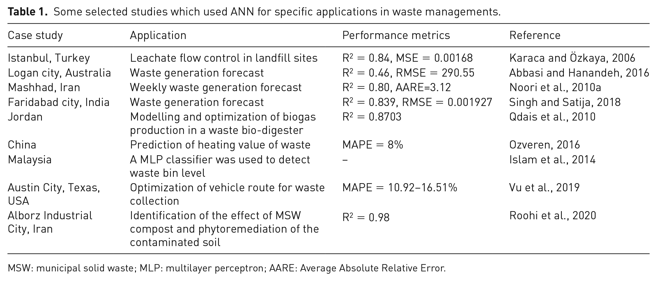
MSW: municipal solid waste; MLP: multilayer perceptron; AARE: Average Absolute Relative Error.
Materials and method
Data set
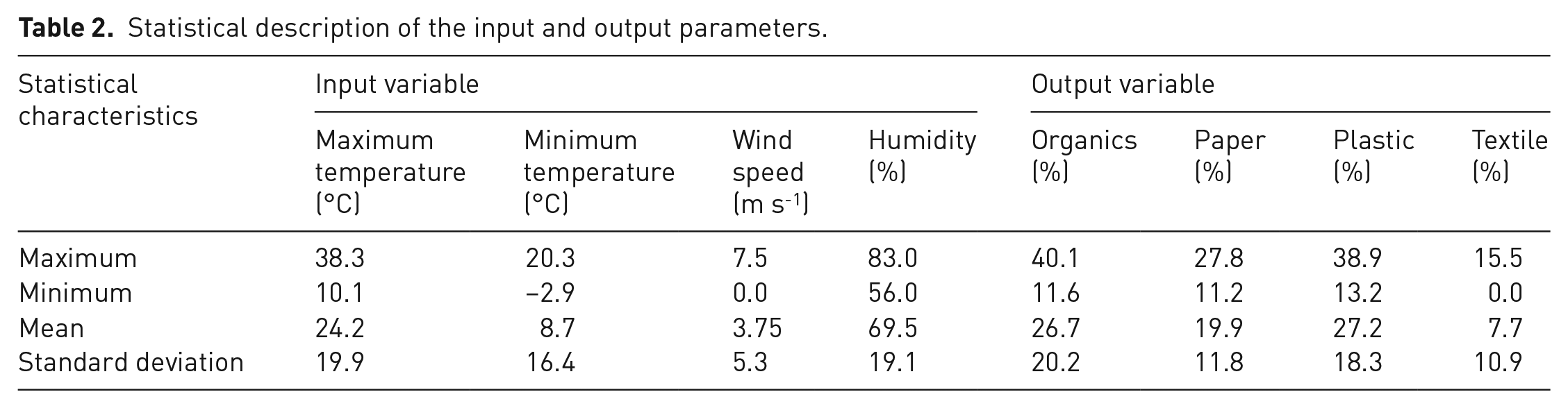
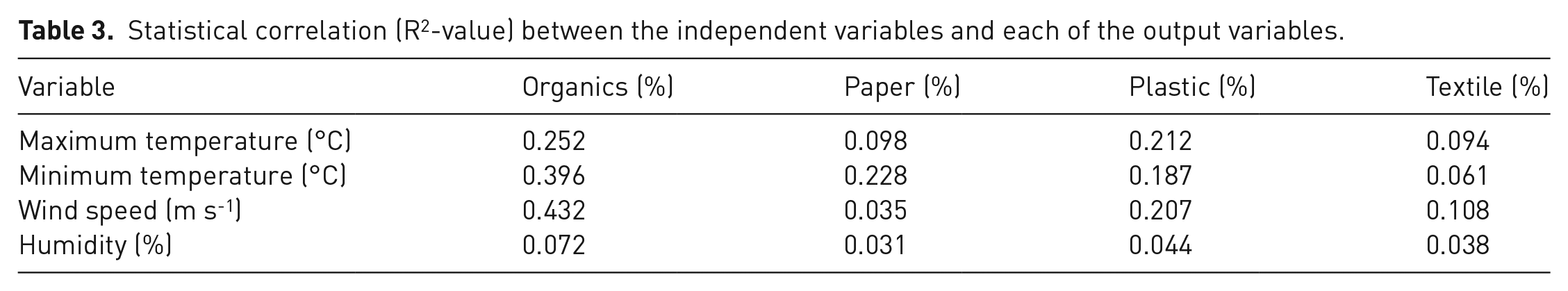
In this study, the model was developed using waste characterization data obtained in summer 2015 and winter 2016 in the city of Johannesburg comprising the percentage composition of organic, paper, plastic and textile waste streams. Four significant meteorological parameters, namely maximum temperature, minimum temperature, humidity and wind speed, for the city of Johannesburg were extracted from South Africa Weather Service for the respective periods of study in 2015 and 2016. Due to the unavailability of experimental waste characterization data in the spring and autumn seasons, the impact of changes in the weather conditions for these two seasons on the physical composition of waste was not considered in this study. Waste collection in Johannesburg is from two different two sources: daily non-compacted (DNC) waste collected from hotels, restaurant and food stores and the round collected refuse (RCR) collected weekly from residential households (Ayeleru et al., 2018). Table 2 presents the statistical properties of the input and output data. The statistical correlation (R2-value) between all the independent variables of the input data and each of the output variables is presented in Table 3.
Statistical description of the input and output parameters.
Statistical correlation (R2-value) between the independent variables and each of the output variables.
Study area
The city of Johannesburg is the constitutional headquarters of South Africa located in the Witwatersrand range of hills (Bwalya, 2019). The city is geospatially located at latitude 26°12’08” S and longitude 28°02’37” E with an area of 1645 km2 and an elevation of 1767 m. The sub-tropical highland weather in Johannesburg produces a mild sunny climate in winter and moderately warm climate in summer. The four major seasons in South Africa generally are winter, summer, autumn and spring. The warmest and wettest month of the year is January, which is in summer, while July, which is in winter, is the driest and coldest month of the year with temperature dropping as low as 4.1°C. Waste management services in the city are operated by the municipality-owned Pikitup Company whose operation capacity is 1.6 million tonnes of MSW collection per annum, with four functional landfill sites (Mbuli, 2015). Figure 1 presents a map of Gauteng showing the major landfill sites in Johannesburg. Based on information available on south database, Statistics South Africa (STATSA), the population and the quantity of waste generated in the city of Johannesburg from 2010 to 2019 is presented in Figure 2. In addition the average values of some of the characteristics of waste generated in the city are presented in Table 4.
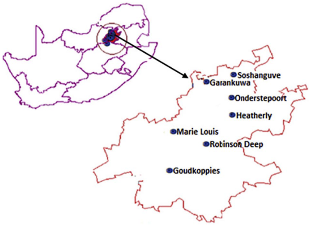
Map of Gauteng showing major landfill sites in Johannesburg.
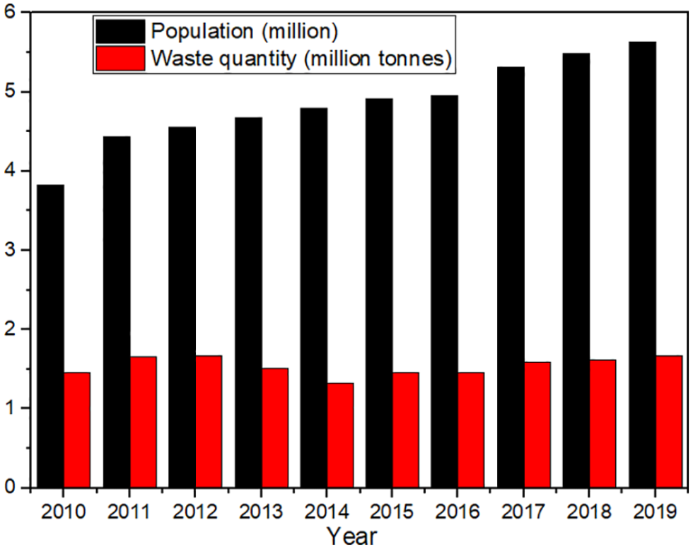
Population and waste quantity generated in the city of Johannesburg (2010–2019).
Some characteristics of waste generated in the city of Johannesburg.
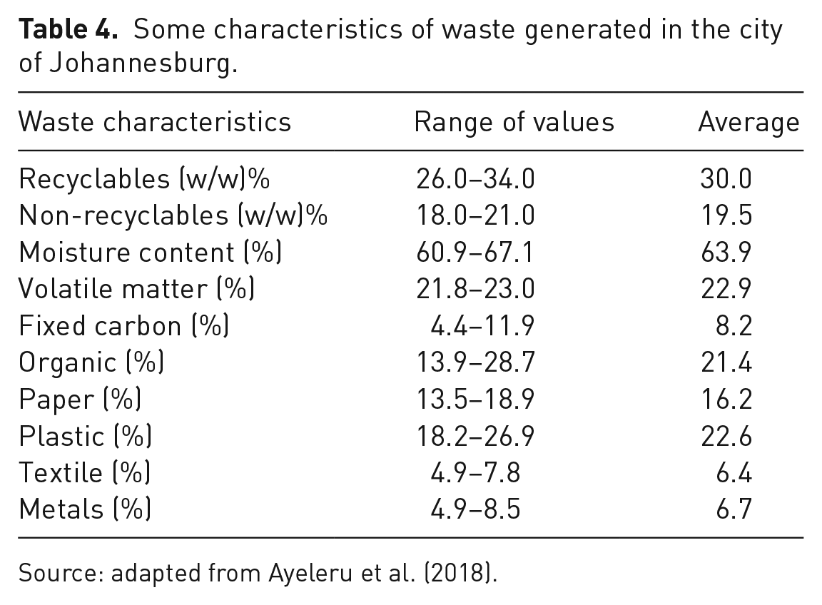
Source: adapted from Ayeleru et al. (2018).
Artificial neural network
Unlike classical programming techniques, ANN works in a similar manner to the human brain by learning from example, making it an excellent self-learning and self-adapting tool which does not require a user-defined solving algorithm (Yaghini et al., 2013). Owing to its approximation capabilities, it is used as an appropriate tool for universal function estimators (Bahrami et al., 2019). ANN is used to approximate functions by adopting iterative procedures focused on error minimization by assigning a weight matrix through the correct choice of AF for solving non-linear processes (Chattopadhyay and Chattopadhyay, 2018). The AF represents the rate of firing in the cell and determines the output from a set of inputs. The neural network can be represented mathematically using equation (2) where the weights and bias assigned to each layer are adjusted.
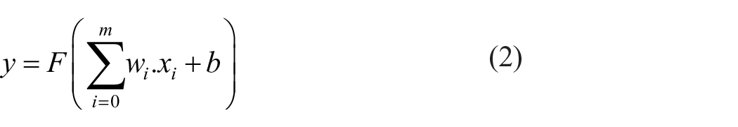
where
The learning rate of the neural network and consequently its performance to a large extent is affected by the AF selected (Ebrahimpour et al., 2008), which could be a linear or non-linear function. Figure 3 shows the architectural structure of the model used in this study
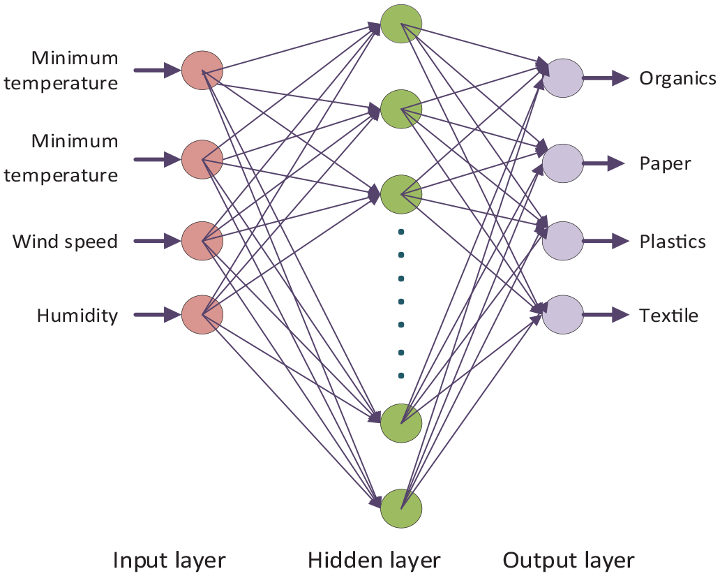
Model architecture consisting of four inputs, several neurons in the hidden layers and four outputs.
Building the optimal neural network
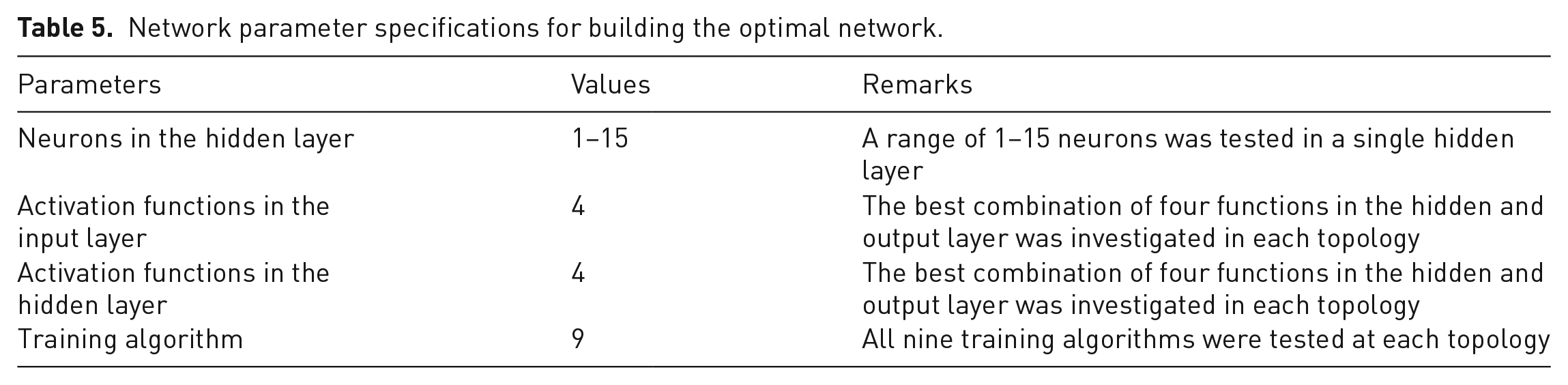
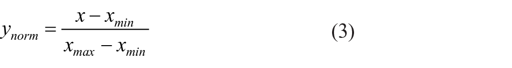
The optimal integration of ANN architecture, AF and TA relies on factors such as the complexity of the desired functions, the size of the input–output datasets and the expected model accuracy and precision, making the choice of best network a difficult task (Bahrami et al., 2019). In this study, the training process was done using ten different TA: namely, Levenberg-Marquardt (LM), scaled conjugate gradient backpropagation (SCG), gradient descent with adaptive algorithm (GDA), Broyden -Fletcher -Goldfarb -Shanno quasi-Newton (BQN), resilient backpropagation (RP), conjugate gradient with Powell/Beale restarts (CGB), conjugate descent backpropagation with Fletcher-Reeves restarts (CGF), conjugate descent with Polak-Ribiere (CGP), one step secant (OSS), variable learning rate backpropagation (VLRB). The AF used at the hidden layers and the output layers are softmax, logsig and tansig and purelin. Table 5 summarizes the parameters of the network which were continuously varied to obtain the optimal network. The dataset was divided into 70% for training and the remaining for testing. The training data was normalized before building the model using equation (3) to ensure that it falls in the same range.
Network parameter specifications for building the optimal network.
where
To obtain the optimal network, several sub-models were stimulated with different topology ranging from 1 to 15 neurons in a single hidden layer. In each topology, 36 sub-models were stimulated by a trial-and-error method through several combinations of the nine TA with all the AF at the hidden and output layers; however the optimal combination for each topology was selected based on minimum error criteria. A single hidden layer was selected because previous research with ANN has proven that a single layer is enough for complex functions approximation (Noori et al., 2010b) and more than one hidden layer is unnecessary (Noori et al., 2011)
Evaluating the model performance
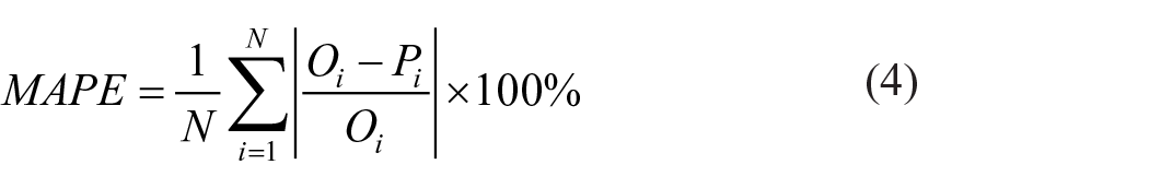
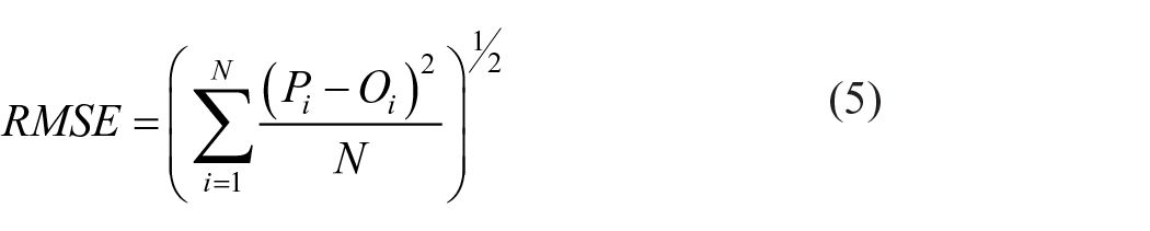
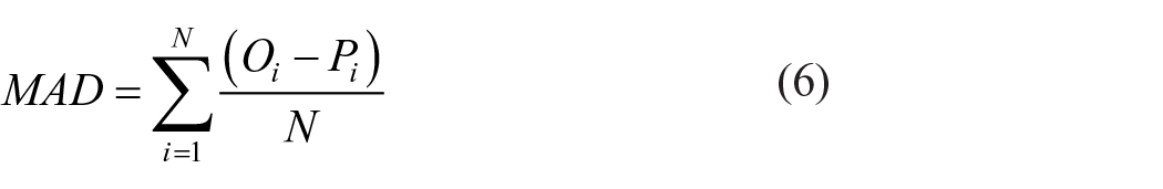
The eligibility and accuracy of the model developed in this study was evaluated using some statistical metrics with the 30% hold-out data for testing. The following statistical metrics were used to evaluation the performance of the models developed for each of the waste streams: root mean square error (RMSE), mean absolute deviation (MAD), mean absolute percentage error (MAPE) and correlation coefficient (R) represented in equations (4) to (6). The RMSE and MAD measures the variability between observed and the predicted values and determines eligibility of the developed model to predict physical waste streams (Olatunji et al., 2019). The correlation coefficient (R) evaluates the agreement between the observed and the predicted waste streams.
Results and discussion
Performance evaluation result
The performance of ANN is influenced by careful choice of hidden layer and neuron numbers, AF and TA. This study has investigated the effect of these parameters on the performance of the models developed and to select the optimal network. The result of the simulation shows that satisfactory models were obtained between 1 and 15 neurons as the model’s performance showed no significant improvement above 15 neurons. More so, a decline was observed in the models performance at two hidden layers, this verifies that waste composition prediction can be done in a single hidden layer. In each topology, 36 sub-models were stimulated with 1–15 neurons in the hidden layer and varied combinations of AF and TA. However, the optimal sub-models in each topology were selected and are presented in this section.
Organic
Performance metrics values of optimal sub-models in each topology are presented in Table 6. It was observed that the performance of these sub-models based on RMSE, MAD and MAPE do not follow a regular trend as the neurons in hidden layer increased from 1 to 15; however an improvement was observed in the R-values as neuron numbers increased up to 10, above which no significant improvement occurred. The optimal network that predicted the organic waste stream was obtained at 10 neurons with the lowest error values (RMSE=3.9293, MAD=2.5738, MAPE=13.0087) and highest R-value of 0.9162 in testing with the combination of softmax and logsig at the hidden and output layer, respectively, and LM. The optimal network is italicized in Table 6. The softmax function outperformed others as its combination mostly at the hidden layer produced more optimal sub-models.
Performance metrics for sub-models in all topology for organic waste.
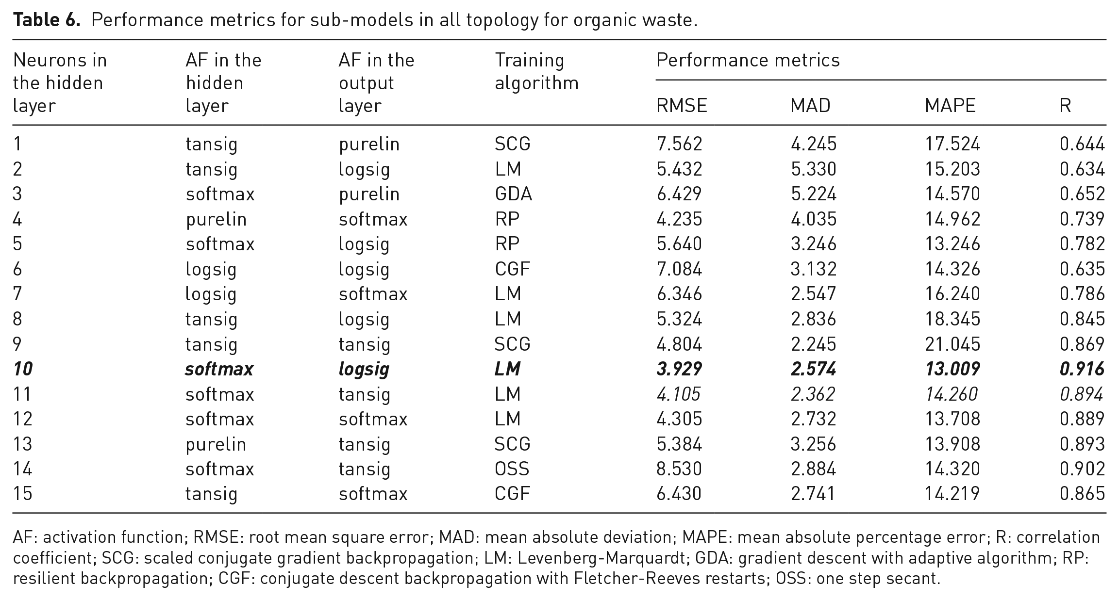
AF: activation function; RMSE: root mean square error; MAD: mean absolute deviation; MAPE: mean absolute percentage error; R: correlation coefficient; SCG: scaled conjugate gradient backpropagation; LM: Levenberg-Marquardt; GDA: gradient descent with adaptive algorithm; RP: resilient backpropagation; CGF: conjugate descent backpropagation with Fletcher-Reeves restarts; OSS: one step secant.
The accuracy of the optimal model is 87% (MAPE=13.008) showing an acceptable fit between the observed and the predicted organic waste while the lower error values of RMSE and MAD show the eligibility of the optimal model in predicting organic waste. The R-value of 0.9162 shows a good agreement between the observed and predicted values. Figure 4 is the test plot of the observed and the predicted organic waste fraction. It further depicts a strong agreement between the observed and predicted values of waste streams with a similar trend between the observed and predicted values. However some under-predictions and over-predictions are observed in the model prediction outcome which are exhibited by some marginal variations in some test samples. This could be attributed to the sensitivity and the response of the model to the extreme and unusual weather parameters recorded on the respective days which represent points of mis-predictions.
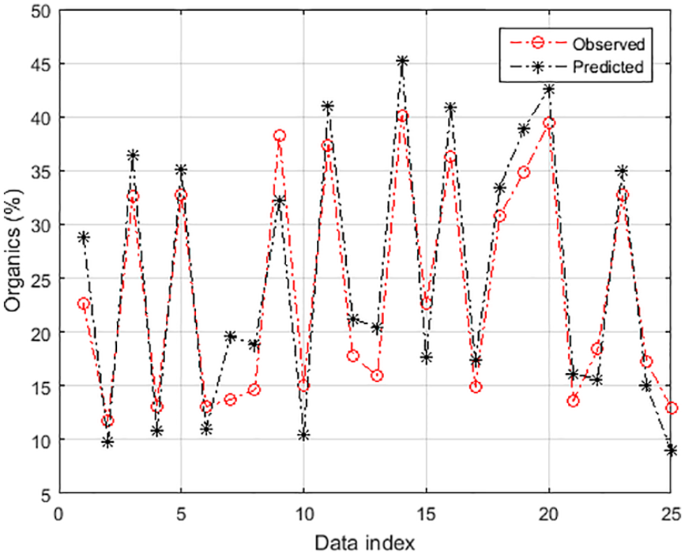
Observed and predicted test sample plot for organic waste.
Paper
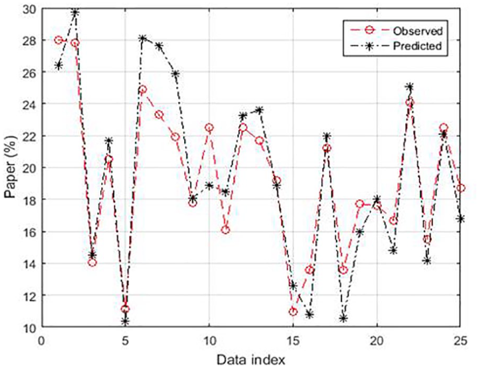
Table 7 presents the performance metrics of the optimal models in each topology for paper waste. An unexpected early convergence at a smaller number of neurons was noticed for prediction of paper waste. The optimal network was obtained at four neurons in the hidden layer with the combination of logsig and purelin at the hidden and output layer and SCG. It was observed that the performance of the sub-models in terms of RMSE, MAD, MAPE and R began to decline at neuron numbers above four. The performance metrics of the optimal network are RMSE=3.243, MAD=3.162, MAPE=17.936 and R=0.862. The accuracy of the optimal network is 82.1% (MAPE=17.936); this depicts a reasonable fit between the observed and predicted paper waste stream. The optimal network was selected based on minimum error values. Based on its RMSE and MAD values showing the variability between the observed and predicted values of paper waste streams, the optimal network model selected is eligible to predict paper waste. The network structure with logsig combinations at either hidden or output layers produced more optimal models in each topology than other functions. All nine TA produced at least one optimal sub-model in each topology; however the SCG-trained network had a higher number of optimal sub-models in each topology. Shown in Figure 5 is the test plot of the observed and the predicted paper waste stream fraction with the optimal model selected. A similar trend is noted between the observed and predicted percentage composition; however, some test samples exhibit marginal variations. This could be attributed to the sensitivity and the response of the model to the extreme and unusual weather parameters recorded on the respective days in the season under study which represent points of over-fitting.
Performance metrics for sub-models in all topology for paper waste.
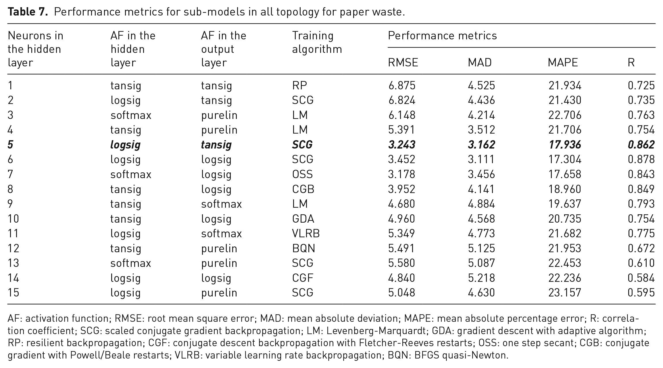
AF: activation function; RMSE: root mean square error; MAD: mean absolute deviation; MAPE: mean absolute percentage error; R: correlation coefficient; SCG: scaled conjugate gradient backpropagation; LM: Levenberg-Marquardt; GDA: gradient descent with adaptive algorithm; RP: resilient backpropagation; CGF: conjugate descent backpropagation with Fletcher-Reeves restarts; OSS: one step secant; CGB: conjugate gradient with Powell/Beale restarts; VLRB: variable learning rate backpropagation; BQN: BFGS quasi-Newton.
Observed and predicted test sample plot for paper waste.
Plastic
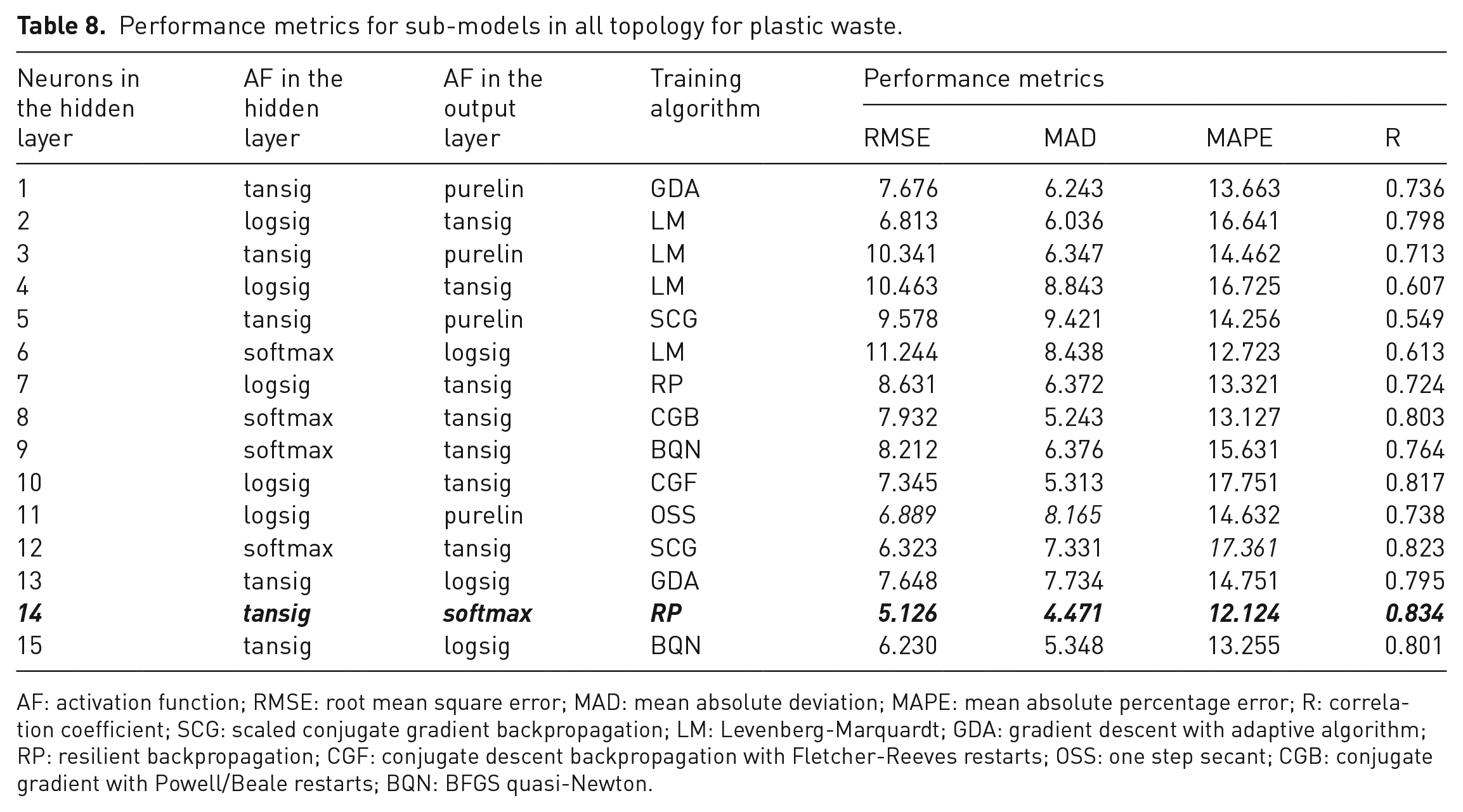
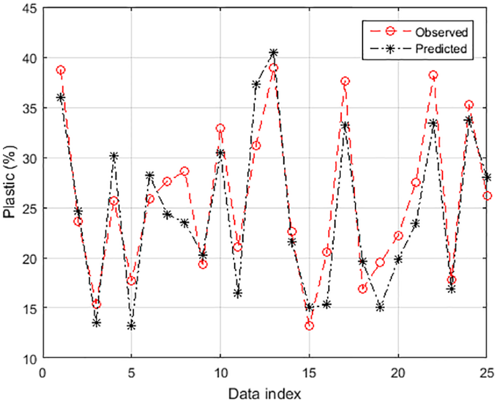
Similar procedures for obtaining the optimal network was followed for plastics waste. Table 8 presents the performance metrics values of the optimal sub-models selected in each topology based on minimum error value and maximum R-values for plastic waste. The optimal model with the minimum error values is a network with 14 neurons in the hidden layer trained with RP algorithms and with tansig and softmax function in the hidden and output layer, respectively. The RMSE and MAD values of the optimal model are 5.126 and 4.471 while the MAPE is 12.124, presenting a model which is 87.9% accurate in mapping an output to the input in the test samples. It was observed that the performances of the sub-models were better at higher numbers of neurons on the hidden layer; however, the performance of the optimal sub-model in each topology does not follow a regular trend as the neuron numbers increase. The RP algorithm trained best to give the overall best network despite the fact that it did not produce the highest number of optimal sub-models. The optimal model is eligible in predicting plastic waste fraction based on the RMSE and MAD values, the MAPE values also depict an acceptable agreement between the observed and predicted plastic waste stream. The observed and predicted value of the plastic waste stream follows a similar trend with no significant variation as presented in Figure 6. The discrepancies at some test samples as earlier noted could be due to the sensitivity and the response of the model predicting plastic waste fraction to the extreme and unusual weather parameters recorded on the respective days in the season under study which represent points of over-fitting and under-fitting.
Performance metrics for sub-models in all topology for plastic waste.
AF: activation function; RMSE: root mean square error; MAD: mean absolute deviation; MAPE: mean absolute percentage error; R: correlation coefficient; SCG: scaled conjugate gradient backpropagation; LM: Levenberg-Marquardt; GDA: gradient descent with adaptive algorithm; RP: resilient backpropagation; CGF: conjugate descent backpropagation with Fletcher-Reeves restarts; OSS: one step secant; CGB: conjugate gradient with Powell/Beale restarts; BQN: BFGS quasi-Newton.
Observed and predicted test sample plot for plastic waste.
Textile
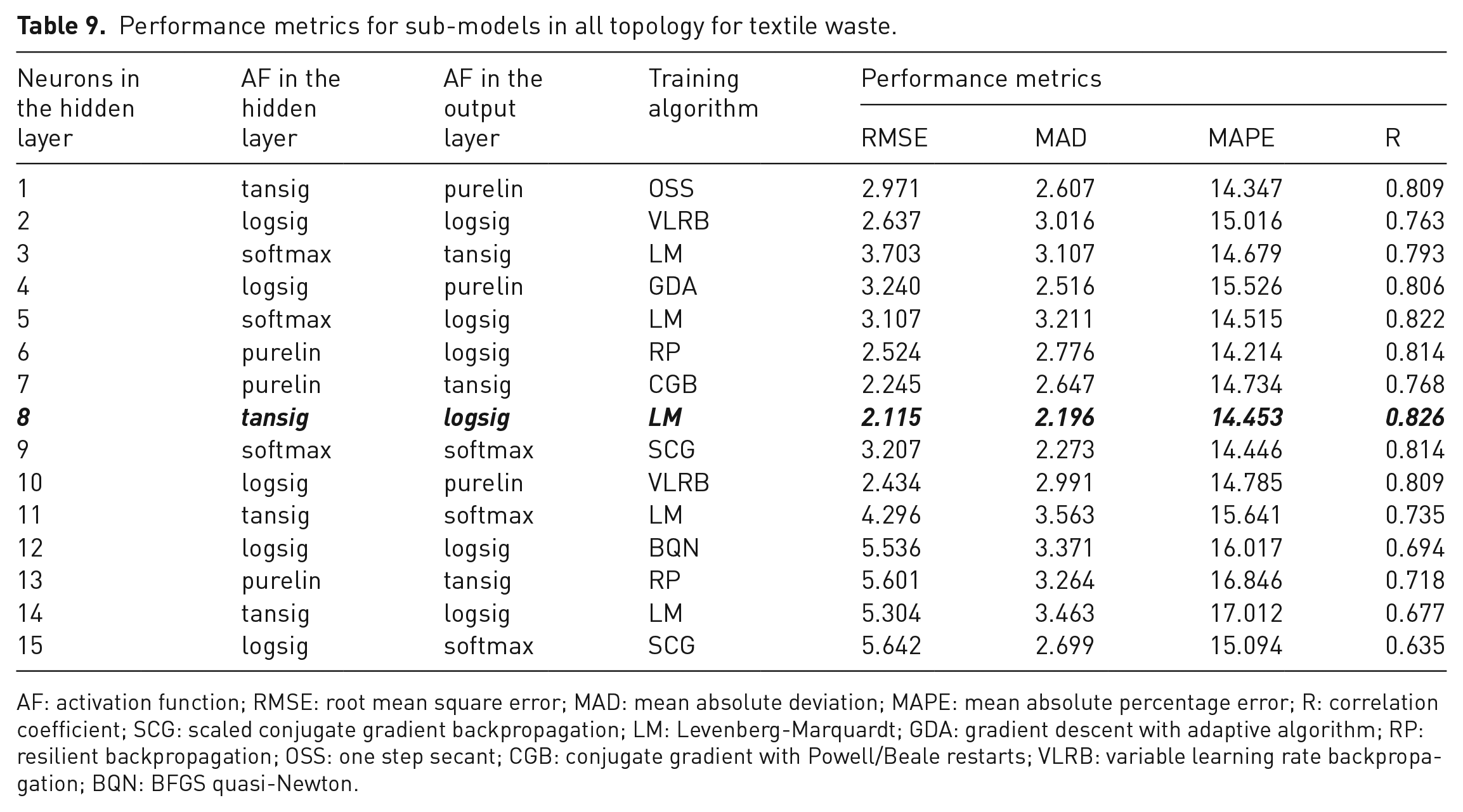
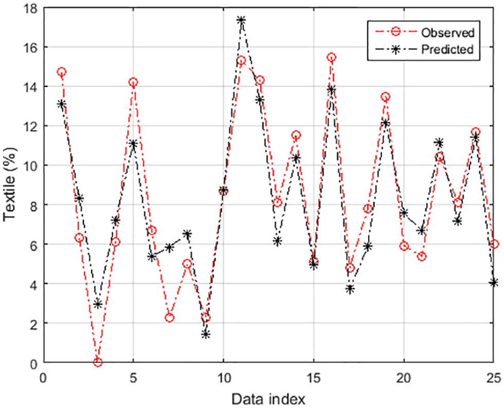
The statistical metrics of sub-models in each topology are presented in Table 9. The performance of the optimal sub-model in each topology was found to improve steadily from 1 to 10 neurons; however an unexpected decline was noticed above 10 neurons. Lower error values, RMSE and MAD were noticed in the model developed for textile waste compared to other outputs; this is because of the relatively lower fraction of textile waste in the total waste. The optimal model based on minimum error values and highest R-values was obtained at eight neurons with tansig and logsig combination at the hidden and output layer and LM algorithm. The RMSE and MAD values of the optimal model are 2.115 and 2.196 while the MAPE is 14.453, presenting a model which is 85.6% accurate in mapping an output to the input in the test samples and depicting an acceptable agreement between the observed and predicted textile waste stream. The observed and predicted value of textile waste fraction in the test plot in Figure 7 follows a similar trend with no significant variation. The response of the models to usual weather parameters on some days in the season could also be accountable for the over-prediction and under-prediction for some test samples. Table 10 compares the performance results of all the optimal models for organic, paper, plastic and textile waste.
Performance metrics for sub-models in all topology for textile waste.
AF: activation function; RMSE: root mean square error; MAD: mean absolute deviation; MAPE: mean absolute percentage error; R: correlation coefficient; SCG: scaled conjugate gradient backpropagation; LM: Levenberg-Marquardt; GDA: gradient descent with adaptive algorithm; RP: resilient backpropagation; OSS: one step secant; CGB: conjugate gradient with Powell/Beale restarts; VLRB: variable learning rate backpropagation; BQN: BFGS quasi-Newton.
Observed and predicted test sample plot for textile waste.
Comparison of the optimal model and parameters for each output.
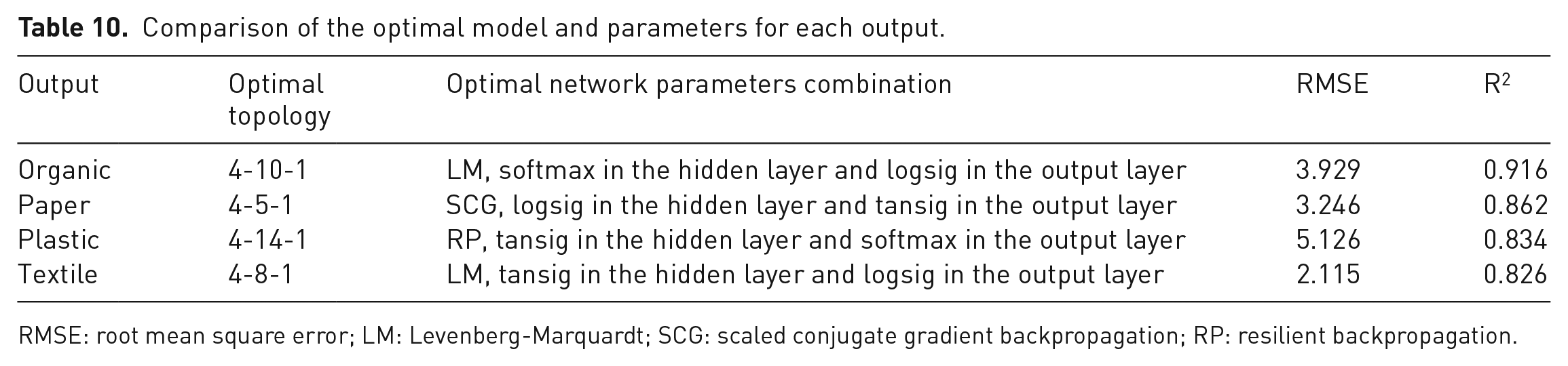
RMSE: root mean square error; LM: Levenberg-Marquardt; SCG: scaled conjugate gradient backpropagation; RP: resilient backpropagation.
Discussion
Waste is collected from two different sources in the city of Johannesburg. DNC waste is collected daily from hotels, restaurants and food stores and the RCR waste is collected weekly from residential households. It was observed that the pattern of variation in the fraction of waste streams from DNC and RCR sources at different seasons vary slightly. This marginal difference can be generally attributed to the different consumption lifestyle of the waste generators from the RCR and DNC sources. The highest observed fraction of organic waste is about 40% which is from the RCR sources in the winter season, while the lowest observed fraction of organic waste was about 12% obtained from the DNC source in the summer season; predicted as 45.1% and 9.8%, respectively. It was observed that the variation in the fractions of organic waste from the DNC source across the seasons is greater than that of the RCR sources. Therefore we can conclude that seasonal variation has more effect on the organic waste fraction of DNC sources than the RCR sources. This is because DNC sources are generated directly from hotels, restaurants and food shops and are collected daily; apparently the daily consumption pattern which produces food waste, fruit and vegetable, and composite waste at those points varies significantly in different seasons.
Waste from the DNC produced the highest paper waste fraction of 27.8% in summer and was predicted as 29.7% while the lowest fraction of paper waste generated was 11.2% from the RCR source in winter and predicted as 10.4%. A wider variation is observed in the fractions of RCR paper waste fractions during the two seasons. It is therefore reasonable to conclude that the changes in climatic conditions in winter and summer influence paper waste streams from the RCR source more than the DNC source. The significant changes in the residential household consumption pattern which affects the quantity of paper packaging, tissue paper and other paper waste generated in different seasons could be attributed to this.
The highest fraction of plastic waste generated was 38.9% from the DNC source in summer and was predicted as 40.5% while the lowest fraction of plastic waste generated was 13.2% from the RCR source in summer and predicted as 15%. Although more plastic waste is generated in summer than in winter from both sources, it was observed that the seasonal variation influences the plastic waste from both DNC and RCR sources in the same manner.
Generally more textile waste is expected to be generated in winter. The highest fraction of textile waste generated was 15.5% from the RCR source in winter and was predicted as 13.8% while the lowest fraction of textile waste generated was 0% from the DNC source in summer and predicted as 2.9%. More textile waste will always be produced from RCR and in winter. This is because more clothing, head coverings and gloves are used for keeping warm in residential spaces, which consequently results in more textile waste. Therefore, the difference in the textile waste from the RCR source in winter and summer is wider than the difference from the DNC source, implying a stronger impact of the changes in weather parameters on RCR textile waste than the DNC textile waste in different seasons.
Conclusion
This study has presented a neural network model to predict the percentage composition of MSW in the city of Johannesburg. Influence of the choice of several network architectures, training algorithms and activation functions on the performance of the models that predict the variability of organic, paper, plastics and textile waste in the winter and summer seasons was evaluated. The best prediction outcome was obtained with a topology 4-10-1, 4-14-1, 4-5-1 and 4-8-1 for organic, paper, plastic and textile waste, respectively. R-values of the optimal network in each topology with the best combinations of AF and TA were 0.916, 0.862, 0.834 and 0.8616, respectively for organics, paper, plastics and textile at the testing phase. Generally, the LM, SCG and RP algorithm had the best performance as they produced at least one optimal model in each output. The result of the study verifies that waste composition prediction can be done in a single hidden layer. The variations in the waste streams for all seasons were generally attributed to the change in consumption patterns, lifestyle adjustment and change in the activities of an individual, household and the municipality at large. It was further revealed that the changes in seasonal weather conditions had more effect on the DNC organic waste than the RCR, while paper from RCR was more impacted by seasonal variation than that from DNC, plastics waste is impacted in the same manner for the DNC and RCR sources while textiles from RCR had a wider difference in percentage composition in both seasons than textiles from DNC.
Footnotes
Acknowledgements
The authors appreciate the management of the Department of Mechanical Engineering Science, University of Johannesburg, South Africa for providing workspace and research facilities for this research.
Declaration of conflicting interests
The authors declared no potential conflicts of interest with respect to the research, authorship, and/or publication of this article.
Funding
The authors received no financial support for the research, authorship, and/or publication of this article.