Kinetic studies on the pyrolysis of plastic waste using a combination of model-fitting and model-free methods

Abstract

In this work, the pyrolysis behavior of plastic waste—TV plastic shell—was investigated, based on thermogravimetric analysis and using a combination of model-fitting and model-free methods. The possible reaction mechanism and kinetic compensation effects were also examined. Thermogravimetric analysis indicated that the decomposition of plastic waste in a helium atmosphere can be divided into three stages: the minor loss stage (20–300°C), the major loss stage (300–500°C) and the stable loss stage (500–1000°C). The corresponding weight loss at three different heating rates of 15, 25 and 35 K/min were determined to be 2.80–3.02%, 94.45–95.11% and 0.04–0.16%, respectively. The activation energy (E_a) and correlation coefficient (R²) profiles revealed that the kinetic parameters calculated using the Friedman and Kissinger–Akahira–Sunose method displayed a similar trend. The values from the Flynn–Wall–Ozawa and Starink methods were comparable, although the former gave higher R² values. The E_α values gradually decreased from 269.75 kJ/mol to 184.18 kJ/mol as the degree of conversion (α) increased from 0.1 to 0.8. Beyond this range, the E_α slightly increased to 211.31 kJ/mol. The model-fitting method of Coats–Redfern was used to predict the possible reaction mechanism, for which the first-order model resulted in higher R² values than and comparable E_α values to those obtained from the Flynn–Wall–Ozawa method. The pre-exponential factors (lnA) were calculated based on the F1 reaction model and the Flynn–Wall–Ozawa method, and fell in the range 59.34–48.05. The study of the kinetic compensation effect confirmed that a compensation effect existed between E_a and lnA during the plastic waste pyrolysis.

Keywords

Plastic waste acrylonitrile-butadiene-styrene pyrolysis kinetics model-free method model-fitting method

Introduction

Once touted as a ‘material of a thousand uses’, plastic meets our demand across various sectors and has become an essential part of daily life (Rahimi and García, 2017). Production and consumption of plastic has increased exponentially since the early 1950s. It is estimated that approximately 400 million tonnes (Mt) of plastic is produced globally each year and a whopping 8300 Mt of plastics was produced between 1950 and 2015 (Geyer et al., 2017). Concomitant with usage, the worldwide generation of plastic waste is rapidly increasing and the amount produced since 2015 is estimated to be 6300 Mt. However, only 9% of this waste has been recycled and 79% has ultimately accumulated in landfill sites or has been dumped in the natural environment (Geyer et al., 2017). It is well known that traditional plastics are difficult to decompose and thus the disposal of plastic waste poses a long-term threat to the natural environment. In order to tackle the plastic disposal problem, the development of alternative recycling or treatment technologies for them is mandatory. Traditional landfilling offers an inexpensive solution for the solid waste, but it will take up land resources and waste the energy intrinsic in plastics (Li et al., 2014). There are drawbacks to recent recycling methods, such as mechanical separation, pelleting and regeneration, attributed to their high labor cost and water contamination (Datta and Kopczyńska, 2016; Deng et al., 2017; Hamad et al., 2013).

Advanced thermal treatments are gaining interest, as these have the advantage of drastic volume reduction and energy recovery (Aguado et al., 2008; Cheng et al., 2019; Yu et al., 2019). Among these, pyrolysis is regarded as one potentially useful method, due to its lower emissions, reasonable cost and simple operation (Qi et al., 2019; Sharuddin et al., 2016). Understanding the process of pyrolysis of plastic waste and its kinetics is important for reactor design and the selection of optimization parameters in practice. Jung et al. (2013) studied the pyrolysis characteristics of waste high impact polystyrene (HIPS) and acrylonitrile-butadiene-styrene (ABS) using a fluidized bed reactor. Szabo et al. (2011) investigated the pyrolysis behavior of a waste polymethylmethacrylate-ABS blend. Liu et al. (2017) investigated the thermal degradation of polymer blends (ABS/polyvinyl chloride (PVC), ABS/nylon 6 (PA6) and ABS/polycarbonate (PC) and analyzed pyrolysis kinetics using the Coats–Redfern (CR) and the Starink methods. Balart et al.(2006) determined the thermal properties of PC-ABS mixtures and studied the kinetics using an autocatalytic model. It is worth noting that reports on the pyrolysis of plastic waste in the form of TV plastic shell are sparse. In addition, it is difficult to precisely describe the pyrolysis kinetics using several methods. Therefore, in this work, a series of thermogravimetric (TG) experiments on plastic waste was conducted using a simultaneous thermal analyzer with different heating rates of 15, 25 and 35 K/min. Based on the TG analysis, the activation energies (E_α) were then determined using four model-free methods, including Friedman, Kissinger–Akahira–Sunose (KAS), Flynn–Wall–Ozawa (FWO) and Starink methods. Finally, the pre-exponential factors (lnA) were analyzed using a combination of the model-fitting method (CR) and model-free methods. The probable mechanism and kinetic compensation effect were investigated as well.

Experimental

Materials

The waste TV plastic shell was collected from a large-scale electrical and electronic equipment recycling plant located in Shandong province, China. It was mainly composed of ABS. It is difficult to crush this plastic using traditional mechanical methods. Therefore, it was ground using a LD-450 cryogenic grinder (Jiangyin Yifang Machinery Co. Ltd., China) with a grinding temperature of −33.1°C.

Experimental procedure

TG analysis is the most widely used technique for studying the thermal decomposition of solids (Ashraf et al., 2019; Bach and Chen, 2017). During the test, approximately 2 mg of the plastic sample was placed on the ceramic crucibles and heated from 20°C to 1000°C under a helium gas flow of 50 mL/min. The tests were repeated at different heating rates of 15, 25 and 35 K/min. The sample weight and temperature changes during the thermal process were recorded to obtain the TG and derivative thermogravimetric (DTG) profiles. The schematic diagram of this study is illustrated in Figure 1.

Figure 1.

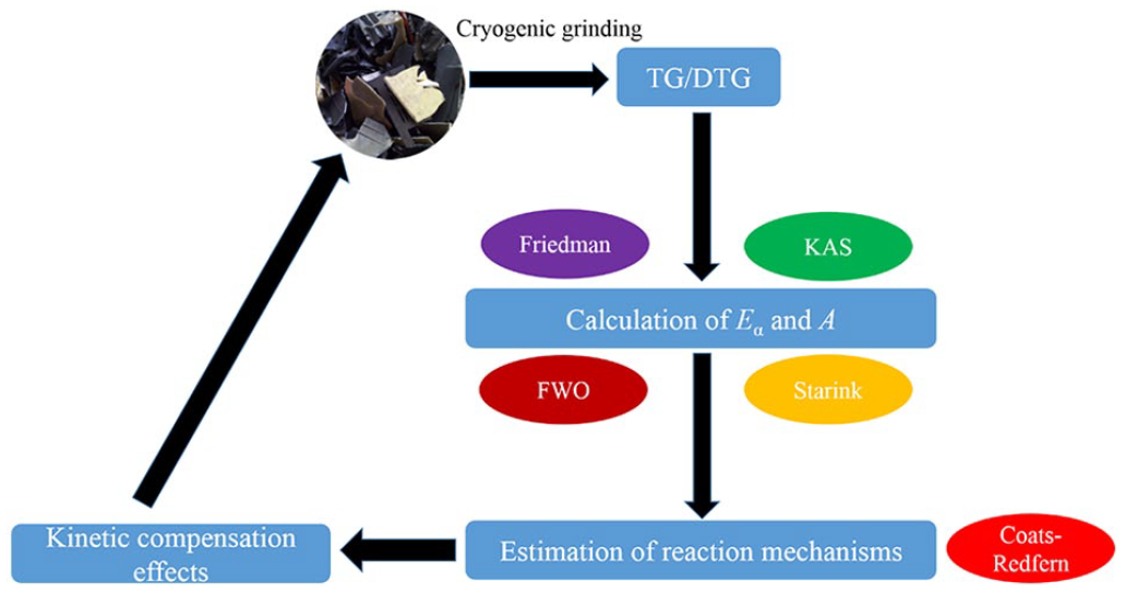
The schematic diagram of this work.

Kinetic modeling

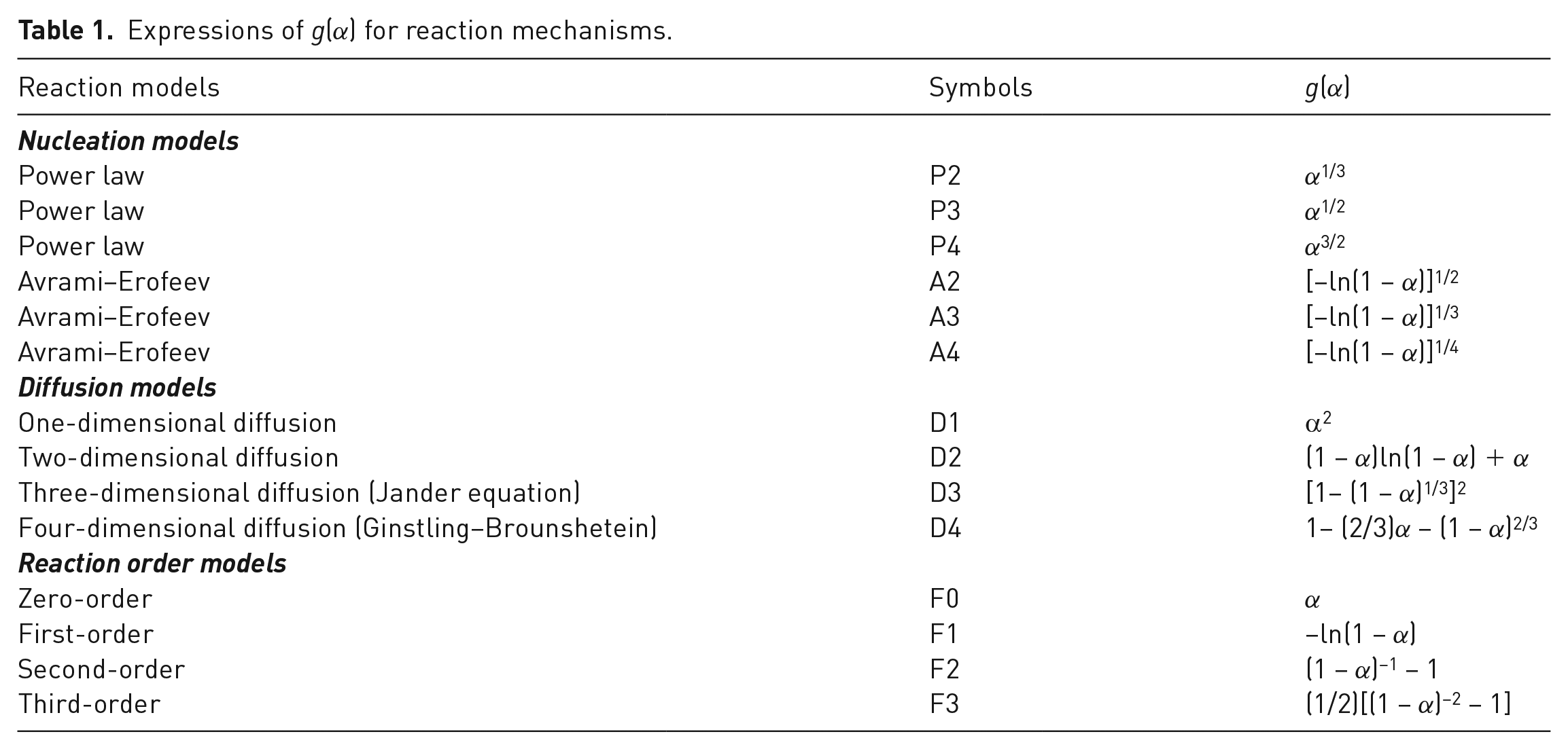
The basic theory of kinetic modeling for solid fuels is presented here; more details can be found elsewhere (Papari and Hawboldt, 2015, Tanaka, 2005, Yao et al., 2019a, Yao et al., 2019b). There are two major methods, the model-fitting and the model-free method, which are employed for the study of the decomposition of solids (Khawam and Flanagan, 2005; Vyazovkin et al., 2011). Model-fitting methods are commonly applied because of their ability to determine the kinetic parameters directly and to offer information about possible reaction mechanisms. Different reaction models have been proposed (Aboulkas and El Bouadili, 2010; Chong et al., 2017; Khawam and Flanagan, 2006; Ma et al., 2018) and kinetic parameters can be determined based on these models. The expressions of g(α) for the different reaction mechanisms used in this work are listed in Table 1. The model-free method does not have any previous assumptions about the reaction model and allows the kinetic parameters to be calculated as a function of the conversion degree. Different model-free methods, such as the Friedman, the FWO, the KAS and the Tang method (Hardi et al., 2018; Srivastava et al., 2017) have been proposed and used for the kinetic study of solid materials. In this work, the model-fitting CR method and the Friedman, FWO, KAS and Starink model-free methods were employed.

Table 1.

Expressions of g(α) for reaction mechanisms.

Reaction models	Symbols	g(α)
Nucleation models
Power law	P2	α ^1/3
Power law	P3	α ^1/2
Power law	P4	α ^3/2
Avrami–Erofeev	A2	[−ln(1 − α)]^1/2
Avrami–Erofeev	A3	[−ln(1 − α)]^1/3
Avrami–Erofeev	A4	[−ln(1 − α)]^1/4
Diffusion models
One-dimensional diffusion	D1	α²
Two-dimensional diffusion	D2	(1 − α)ln(1 − α) + α
Three-dimensional diffusion (Jander equation)	D3	[1− (1 − α)^1/3]²
Four-dimensional diffusion (Ginstling–Brounshetein)	D4	1− (2/3)α − (1 − α)^2/3
Reaction order models
Zero-order	F0	α
First-order	F1	−ln(1 − α)
Second-order	F2	(1 − α)⁻¹ − 1
Third-order	F3	(1/2)[(1 − α)⁻² − 1]

The TG results can be expressed as a function of degree of conversion (α), which is defined in terms of mass change for solids as

α = \frac{m_{0} - m_{t}}{m_{0} - m_{f}}

(1)

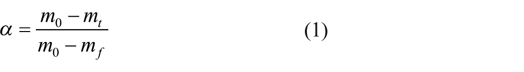
where m₀ and m_f refer to the initial and final sample weight, and m_t represents the instantaneous mass at time t.

The solid conversion rate (dα/dt) can be expressed as

\frac{d α}{d t} = β \frac{d α}{d T} = κ (T) \times f (α)

(2)

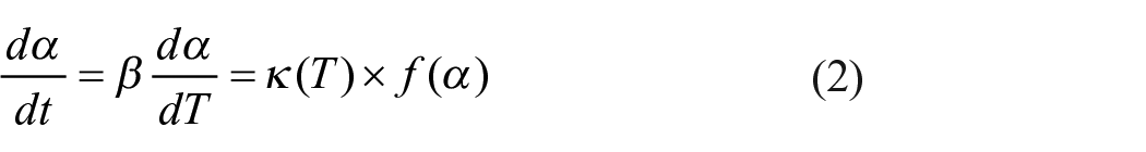
where β is the heating rate or the rate of temperature change (dT/dt, K/min), κ(T) refers to the reaction rate constant depending on the temperature and f(α) represents the kinetic model function.

The κ(T) can be described according to the Arrhenius equation

κ (T) = A e^{- \frac{E}{R T}}

(3)

where A refers to the pre-exponential factor (min⁻¹), E is the apparent activation energy (kJ/mol) and T and R represent the absolute temperature (K) and universal gas constant (8.314 J/(mol·K)), respectively.

Under constant temperature ramp conditions, combining equation (2) and equation (3) yields

\frac{d α}{d T} = \frac{A}{β} e^{- \frac{E}{R T}} f (α)

(4)

CR method

The CR method is an integral model-fitting method developed by Coats and Redfern (1964), which uses an asymptotic series expansion for estimation of the temperature integral. The integral form of the reaction model can be obtained by integrating equation (4) as (Çepelioğullar et al., 2016; Özveren and Özdoğan, 2013)

\begin{array}{l} g (α) = \int \overset{α}{0} \frac{d α}{f (α)} = \frac{A}{β} \int \overset{T}{0} e^{- \frac{E}{R T}} d T \\ = \frac{A E}{β R} \int \overset{\infty}{x} \frac{e^{- x}}{x^{2}} d_{x} = \frac{A E}{β R} p (x) \end{array}

(5)

where x is equal to $\frac{E}{R T}$ . The p(x) is the temperature integral and has no analytical solution. Therefore, equation (5) can only be solved using either numerical integration or approximation in order to deal with the complex integral. The distinction between the various model-free methods is attributed to the type of approximation employed.

By introducing an approximation $p (x) = x^{- 2} e^{- x}$ (20 ⩽ x ⩽ 50) into equation (5), the relationship between heating rate and inverse temperature becomes

g (α) = \frac{A R T^{2}}{β E} (1 - \frac{2 R T}{E}) e^{- \frac{E}{R T}}

(6)

Taking the natural logarithm of both sides of equation (6) yields

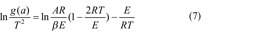
\ln \frac{g (a)}{T^{2}} = \ln \frac{A R}{β E} (1 - \frac{2 R T}{E}) - \frac{E}{R T}

(7)

Since 2RT/E << 1, the equation can be converted into

\ln \frac{g (a)}{T^{2}} = \ln \frac{A R}{β E} - \frac{E}{R T}

(8)

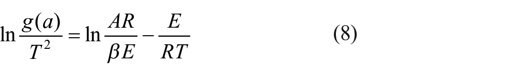
For a fixed β and proposed reaction mechanism g(α), plotting $\ln \frac{g (a)}{T^{2}}$ versus $\frac{1}{T}$ gives a straight line. The slope −E/R and intercept $\ln \frac{A R}{β E}$ can be used to determine E and A, respectively.

Friedman method

Both differential and integral isoconversional methods were used for determination of the activation energy. The Friedman method (Friedman, 1964) is the most common differential isoconversional method for evaluating the activation energy as a function of α. It is based on the assumption that the decomposition of the solids depends only on the rate of mass loss and is independent of the temperature. Therefore, the f(α) can be considered constant and taking the natural logarithms of both sides of equation (4) yields

l n (β \frac{d α}{d T}) = l n [A f (α)] - \frac{E_{α}}{R T}

(9)

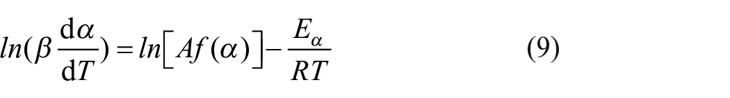
A series of TG experiments at different heating rates enables the extraction of data for the same α value at different temperatures (Özveren and Özdoğan, 2013). Because ln[Af(α)] is a constant, for given α and β values, the activation energy can be determined from the slope of the straight line by plotting $\ln (β \frac{d α}{d T})$ versus $\frac{1}{T}$ .

KAS method

The integral term p(x) in equation (5) has no analytical solution. All the integral isoconversional methods are based on different mathematical assumptions of p(x). The KAS method (Akahira and Sunose, 1971) is based on the CR approximation $p (x) = x^{- 2} e^{- x}$ (20 ⩽ x ⩽ 50) and equation (8) can be converted into

\ln \frac{β}{T^{2}} = \ln \frac{A R}{E_{α} g (α)} - \frac{E_{α}}{R T}

(10)

For a constant value of α, the activation energy can be obtained from the plot of $\ln \frac{β}{T^{2}}$ against $\frac{1}{T}$ with −E_α/R as the slope.

FWO method

The FWO method is a model-free method developed by Flynn and Wall (1966) as well as Ozawa (1965). It uses Doyle’s equation for the approximation of the temperature integral (Doyle, 1965). Taking into account the approximation $\ln p (x) = - 5.331 - 1.052 x$ , equation (5) can be converted into

\ln β = \ln \frac{A E_{α}}{R g (α)} - 5.331 - 1.052 \frac{E_{α}}{R T}

(11)

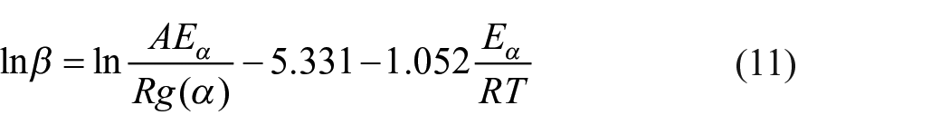
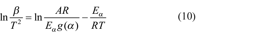
For a fixed value of α, plotting lnβ versus 1/T gives a straight line. The activation energy can be determined from the slope −1.052E_α/R over a series of α. The A values can be obtained from the intercept, $\ln \frac{A E}{R g (α)} - 5.331$ , after obtaining the E_α values and selecting g(α) from Table 1.

Starink method

By integrating the approximation $p (x) = \frac{e^{- 1.0008 x - 0.312}}{x^{1.92}}$ into equation (8), the relationship between heating rate and inverse temperature becomes

\ln \frac{β}{T^{1.92}} = - 1.0008 \frac{E_{α}}{R T} + C

(12)

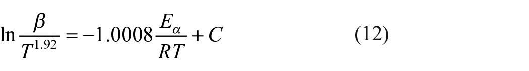
For a series of α, numerous pairs of $\ln \frac{β}{T^{1.92}}$ and 1/T can be extracted at several heating rates. The plot of $\ln \frac{β}{T^{1.92}}$ versus $\frac{1}{T}$ should give a straight line and the slope −1.0008E_α/R can be used to calculate E_α.

Results and discussion

TG analysis

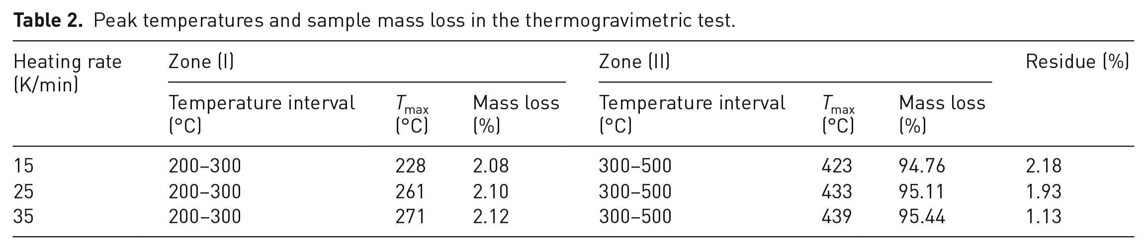
The conversion rate and DTG curves of plastic waste at different heating rates are displayed in Figure 2. From Figure 2(a), it can be seen that the conversion displayed a similar trend for samples at different heating rates. The whole thermal process can be divided into three stages: the minor loss stage (20–300°C), the major loss stage (300–500°C) and the stable loss stage (500–1000°C). The weight loss at three heating rate were determined to be 2.80–3.02%, 94.45–95.11% and 0.04–0.16% for these stages, respectively, which was consistent with the decomposition of ABS polymer (Ma and Pang, 2015; Polli et al., 2009). As for the thermal degradation of pure ABS, some researchers observed one or two steps. The discrepancy mainly derives from the sample molecular weight, sample mass, heating rate, etc. From the DTG profiles in Figure 2(b), it was found that the DTG curve can be divided into three zones. Among them, zone I is the initiation of pyrolysis, during which the backbone of the polymer ruptured into monomers, such as styrene, acrylonitrile and polybutadiene (Yang et al., 2004, Yu et al., 2019). Suzuki and Wilkie (1995) investigated the degradation of pure ABS and found that the evolution of butadiene commenced at 340°C and styrene at 350°C, while the evolution of monomeric acrylonitrile initiated at 400°C. Zone II is the major conversion stage, where a significant mass loss of approximately 95% was observed. The decomposition rates elevated from 0.12 to 0.28 %•s⁻¹ with the heating rate increasing from 15 to 35 K/min. In this stage, monomers resulting from zone I decomposed to form small molecules, such as HBr, CO₂, CO and CH₄ (Yu et al., 2019). In zone III, the degradation rate significantly decreased to 2.13E⁻⁵–55.05E⁻⁵ %•s⁻¹ and a minor weight loss of 0.04–0.40% was observed. Larger brominated derivatives decomposed and smaller molecules dominated the major gaseous products (Yu et al., 2019). This indicated that the decomposition of TV plastic shell was mainly occurred at less than 500°C, namely, in zone I and zone II. From Figure 2 and Table 2, the maximum peak temperatures were observed at 228, 261 and 271°C for three heating rates in zone I and 423, 433 and 439 °C in zone II, respectively. The obvious shift toward higher peak decomposition temperatures with increasing heating rate has been reported in the literature for coal (Song et al., 2016) and biomass (Cortés and Bridgwater, 2015). This may be attributed to the increasing effect of heat transfer limitations, which cause temperature gradients within the sample and inside each particle. At a lower heating rate, the heating of plastic particles occurs gradually leading to an improved heat transfer to the inner portions and among the particles. However, an increase of T_max is also observed if there is no limitation of heat transfer (Kissinger, 1956). The increase of T_max upon increasing heating rate can be seen from equations (8) to (12), which all assume ideal heat transfer (without any temperature gradients in the interior of the particles or the sample). Therefore, zone II was selected to study the pyrolysis kinetics of plastic waste in the following section.

Figure 2.

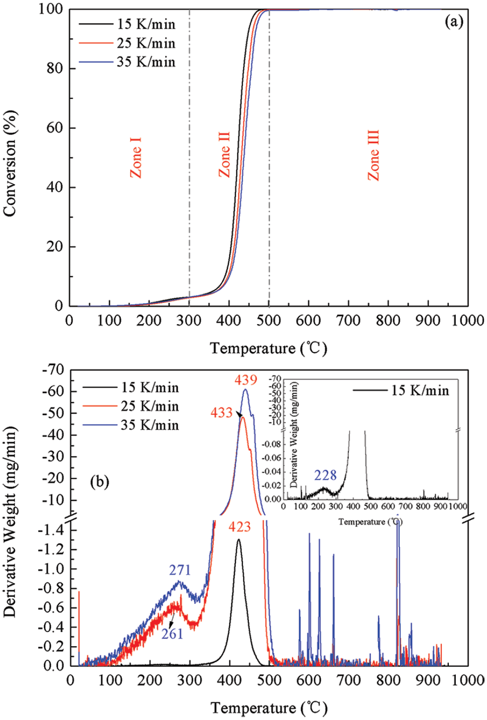
(a) Conversion rate and (b) derivative thermogravimetric (DTG) curves of plastic waste at different heating rates.

Table 2.

Peak temperatures and sample mass loss in the thermogravimetric test.

Heating rate(K/min)	Zone (I)			Zone (II)			Residue (%)
Heating rate(K/min)	Temperature interval(°C)	T_max (°C)	Mass loss(%)	Temperature interval(°C)	T_max (°C)	Mass loss(%)	Residue (%)
15	200–300	228	2.08	300–500	423	94.76	2.18
25	200–300	261	2.10	300–500	433	95.11	1.93
35	200–300	271	2.12	300–500	439	95.44	1.13

Calculation of activation energy

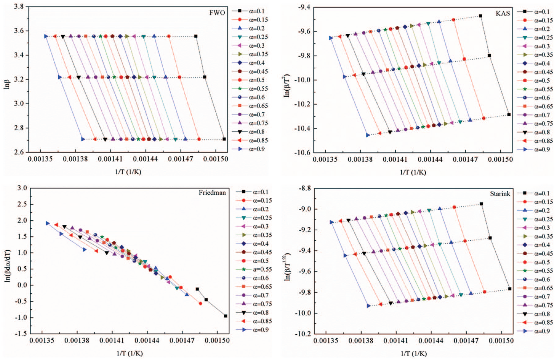
In this section, the activation energy (E_α) and linear correlation coefficient (R²) at various conversion rates of 0.1–0.9 were calculated using the Friedman, KAS, FWO and Starink methods. For the Friedman method, the plots of $\ln (β \frac{d α}{d T})$ against $\frac{1}{T}$ yielded straight lines for each α with slopes directly proportional to E (Figure 3). The calculated E_α and R² are shown in Table 3. It was obvious that the E_α values fluctuated significantly in the range of 162.92–344.64 kJ/mol.

Figure 3.

The linear fitting curves under different conversions for model-free methods.

Table 3.

The kinetic parameters determined using the model-free methods.

α	Friedman			Flynn–Wall–Ozawa			Kissinger–Akahira–Sunose			Starink
α	E(kJ/mol)	R	lnA	E(kJ/mol)	R	lnA	E(kJ/mol)	R	lnA	E(kJ/mol)	R
0.1	278.22	0.9894	49.47	269.747	0.9898	46.83	222.557	0.9943	38.07	272.880	0.9890
0.15	261.20	0.9979	46.10	256.304	0.9979	44.06	258.341	0.9977	44.37	258.591	0.9978
0.2	254.35	0.9989	44.79	250.131	0.9990	42.87	337.058	0.9864	58.40	252.012	0.9989
0.25	245.82	0.9974	43.24	242.671	0.9952	41.50	243.841	0.9948	41.66	244.103	0.9948
0.3	239.71	0.9998	42.15	236.649	0.9998	40.42	220.895	0.9948	37.58	237.723	0.9998
0.35	234.11	0.9998	41.15	230.303	0.9994	39.30	230.722	0.9993	39.34	230.994	0.9993
0.4	228.35	1.0000	40.13	228.200	0.9999	38.94	220.421	0.9949	37.58	228.743	0.9999
0.45	219.88	0.9999	38.64	214.251	0.9998	36.49	213.745	0.9998	36.36	214.039	0.9998
0.5	212.84	1.0000	37.39	212.84	0.9998	35.40	219.257	0.995	37.40	207.451	0.9998
0.55	210.16	0.9985	36.90	205.590	0.9984	35.00	204.558	0.9982	34.77	204.859	0.9982
0.6	200.33	0.9996	35.18	199.599	0.9991	33.95	218.608	0.9946	37.29	198.521	0.999
0.65	193.28	1.0000	33.93	191.182	0.9999	32.49	189.310	0.9998	32.11	189.632	0.9999
0.7	188.33	1.0000	33.03	187.286	1.0000	31.83	165.490	0.986	28.00	185.487	1.0000
0.75	186.31	0.9999	32.30	185.714	0.9998	31.54	183.448	0.9998	31.07	183.775	0.9998
0.8	184.60	0.9990	32.21	184.180	0.9991	31.26	157.708	0.9732	26.63	182.114	0.9990
0.85	194.67	0.9986	33.76	193.735	0.9987	32.86	191.762	0.9985	32.46	192.091	0.9985
0.9	212.86	0.9991	36.58	211.311	0.9992	35.79	166.538	0.9864	28.16	210.483	0.9991

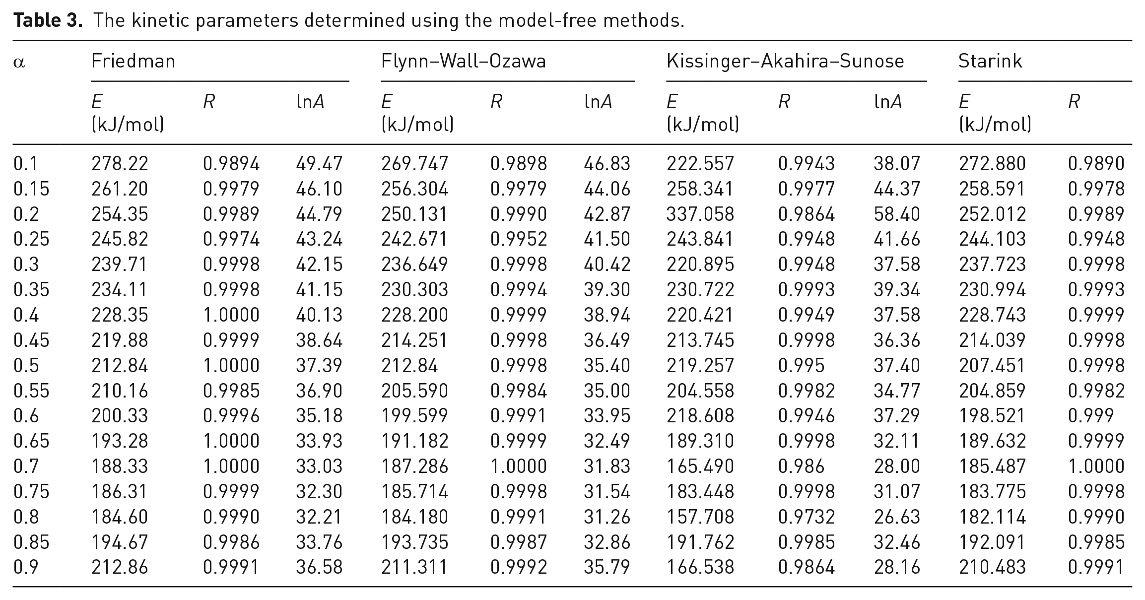
The kinetic parameters calculated using the KAS method displayed a similar trend to those from the Friedman method, although they were smaller than the latter (Figure 4). This was consistent with the literature (Yuan et al., 2017), although an increasing tendency with an increase of α was displayed. Pérez et al. (2012), reported that E_α values from the KAS method became larger than those from the Friedman method for α >0.65. In other literature (Sokoto and Bhaskar, 2018), the activation energy calculated using the Friedman method decreased with increasing α in the range 0.1–0.6, while the values derived from the KAS method were stable for α values of 0.1–0.15 and 0.2–0.4. A decrease in E_α values was observed for α values of 0.4–0.6.

Figure 4.

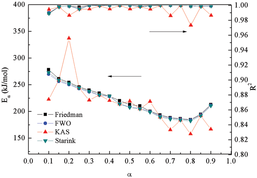
Comparison of kinetic parameters derived from model-free methods.

The FWO method is an integral method, which is also independent of the degradation mechanism. According to equation (11), numerous pairs of lnβ and 1/T data at various α values of 0.1–0.9 were plotted and displayed in Figure 3. The activation energies were then calculated by the slopes (−1.052E_α/R) and listed in Table 3. Unlike the above two methods, this manifested a noticeable decreasing trend. The E_α values gradually decreased from 269.75 kJ/mol to 184.180 kJ/mol with an increase in α from 0.1 to 0.8. Beyond this range (α > 0.8), the E_α values increased slightly to 193.74 kJ/mol and 211.31 kJ/mol for α values of 0.85 and 0.9, respectively. Therefore, the entire variation of E_α can be divided into region I (< 0.8) and region II (> 0.8) according to the conversion rate. The average values of E_α were determined to be 219.32 kJ/mol and 202.52 kJ/mol for regions I and II, respectively.

The kinetic parameters calculated using the Starink method displayed the same trend as those derived from the FWO method. This was consistent with the literature (Wu et al., 2018), although the activation energy displayed three stages for the entire α range of 0.05–0.95.

When the four model-fitting methods are compared, similar activation energies and correlation coefficients were observed for the Friedman and KAS methods. The profiles are displayed for these and for the other two methods in Figure 4. However, the E_α and R² values determined from Friedman and KAS fluctuated significantly, so the FWO and Starink methods were shown to be more accurate for probing the pyrolysis kinetics. Comparing the two methods, higher R² values were derived from the FWO method for an α range of 0.1–0.9. Therefore, the FWO was the most reliable method and this was used for the reaction mechanism study in the following section.

Estimation of reaction mechanisms

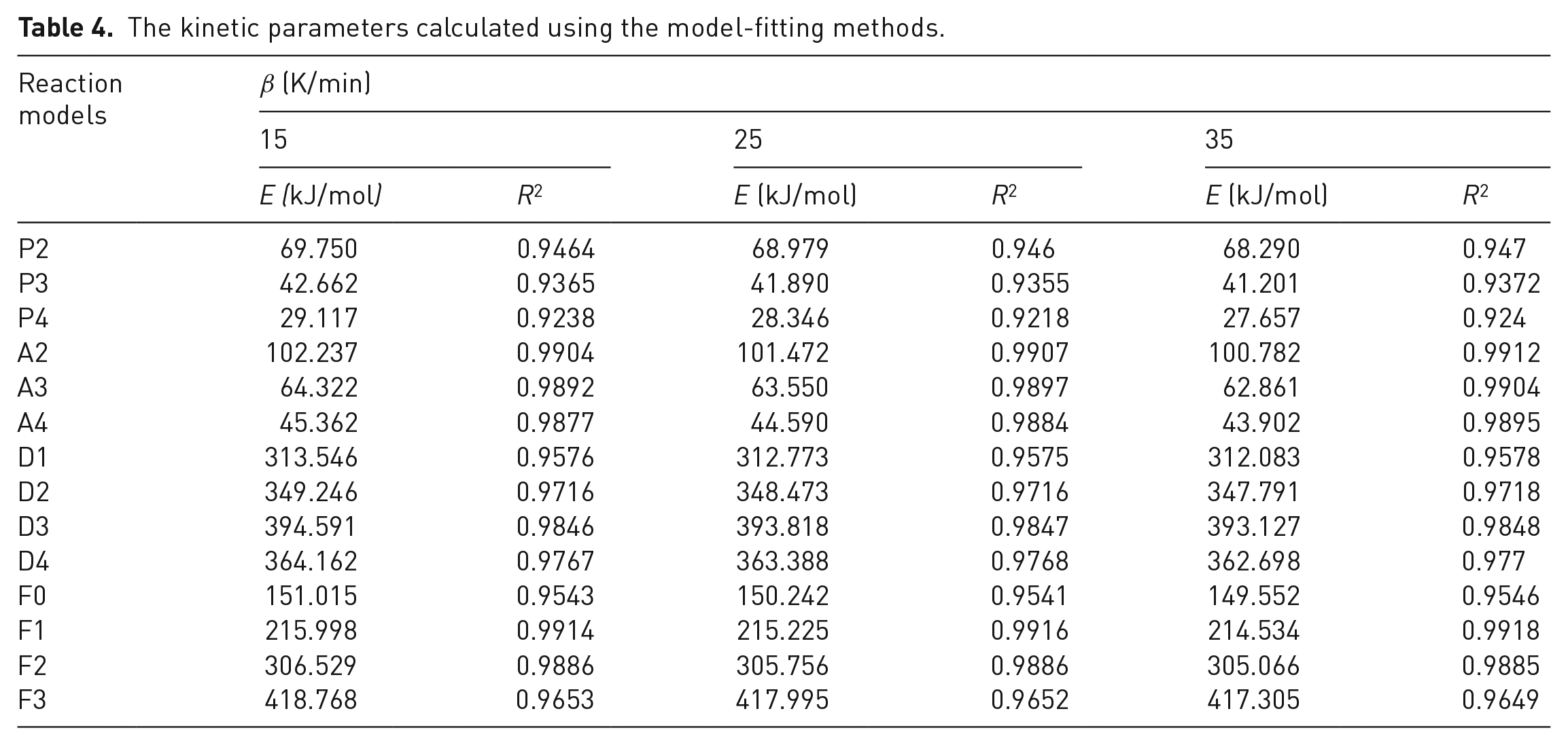
Employment of the CR method for TG data can determine the most probable mechanism function and enable the pre-exponential factor (lnA) to be calculated (Aboulkas and El Bouadili, 2010; Ding et al., 2017). If the average E_α values for three heating rates based on a certain mechanism are comparable to the values from the FWO method, then this mechanism could be responsible for the reaction. From equation (8), the activation energy for all g(α) functions listed in Table 1 can be obtained. The resulting kinetic parameters are listed in Table 4 and displayed in Figure 5. For each model, the E_α values decreased with the increase of heating rate. The E_α and R² values can be used as criteria for determining the most reliable reaction models. It was obvious that the E_α and R² values fell into the range of 25.24–418.77 kJ/mol and 0.9238–0.9969, respectively. In addition, the three groups of reaction models displayed distinct profiles. The diffusion models gave larger E_α values, while the nucleation models gave lower values. The F1 model resulted in higher R² values and the calculated E_α values were 216.00, 204.60 and 194.66 kJ/mol at the three heating rates; these were close to the average E_α values of 219.32 kJ/mol and 202.52 kJ/mol for regions I and II derived from the FWO method. Therefore, the most appropriate mechanism for plastic waste pyrolysis can be regarded to be the first-order reaction model (Dou et al., 2007).

Table 4.

The kinetic parameters calculated using the model-fitting methods.

Reaction models	β (K/min)
	15		25		35
	E (kJ/mol)	R ²	E (kJ/mol)	R ²	E (kJ/mol)	R ²
P2	69.750	0.9464	68.979	0.946	68.290	0.947
P3	42.662	0.9365	41.890	0.9355	41.201	0.9372
P4	29.117	0.9238	28.346	0.9218	27.657	0.924
A2	102.237	0.9904	101.472	0.9907	100.782	0.9912
A3	64.322	0.9892	63.550	0.9897	62.861	0.9904
A4	45.362	0.9877	44.590	0.9884	43.902	0.9895
D1	313.546	0.9576	312.773	0.9575	312.083	0.9578
D2	349.246	0.9716	348.473	0.9716	347.791	0.9718
D3	394.591	0.9846	393.818	0.9847	393.127	0.9848
D4	364.162	0.9767	363.388	0.9768	362.698	0.977
F0	151.015	0.9543	150.242	0.9541	149.552	0.9546
F1	215.998	0.9914	215.225	0.9916	214.534	0.9918
F2	306.529	0.9886	305.756	0.9886	305.066	0.9885
F3	418.768	0.9653	417.995	0.9652	417.305	0.9649

Figure 5.

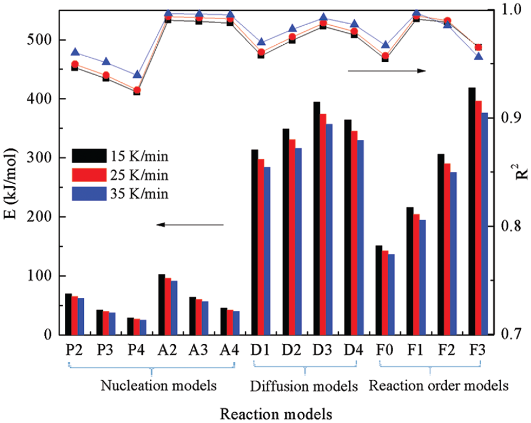
Comparison of kinetic parameters calculated from model-fitting methods.

Kinetic compensation effects

The kinetic compensation effect is usually used to characterize the dependence of E and A on the conversion degree according to the following linear relationship (Wang et al., 2012; Zhu et al., 2015)

\ln A = a E + b

(13)

where a and b are constants and refer to the compensation coefficients.

The F1 mechanism was selected for determining the pre-exponential factors as a function of conversion to validate the kinetic parameter. The activation energy calculated using the FWO method was more reliable and was used in this section. Substituting $f (a) = - l n (1 - α)$ into equation (11) yields

\ln β = \ln \frac{A E_{α}}{- R \ln (1 - α)} - 5.331 - 1.052 \frac{E_{α}}{R T}

(14)

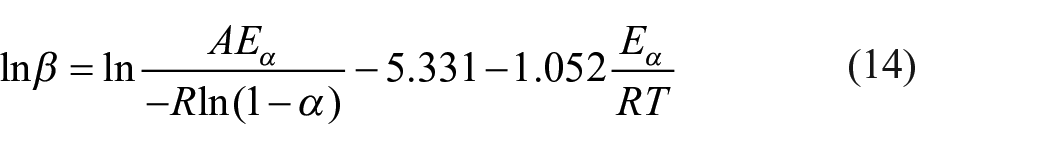
From the Eα values determined using the FWO method in Table 3, the lnA values can be calculated according to equation (14). An excellent linear relationship, lnA = 0.1832E + 9.551 (R² = 0.9993), can be found through plotting lnA against E, as shown in Figure 6. It indicated that compensation effect existed between the apparent E_α and lnA during the pyrolysis of plastic waste. The lnA fell into the range of 59.34–48.05 with α increasing from 0.1 to 0.9, which can be confirmed by Table 3. Therefore, the kinetic compensation effect was a valid alternative to demonstrating the interrelationship between the kinetic parameters lnA and E due to the impact of the experimental conditions on the determination of kinetic parameter.

Figure 6.

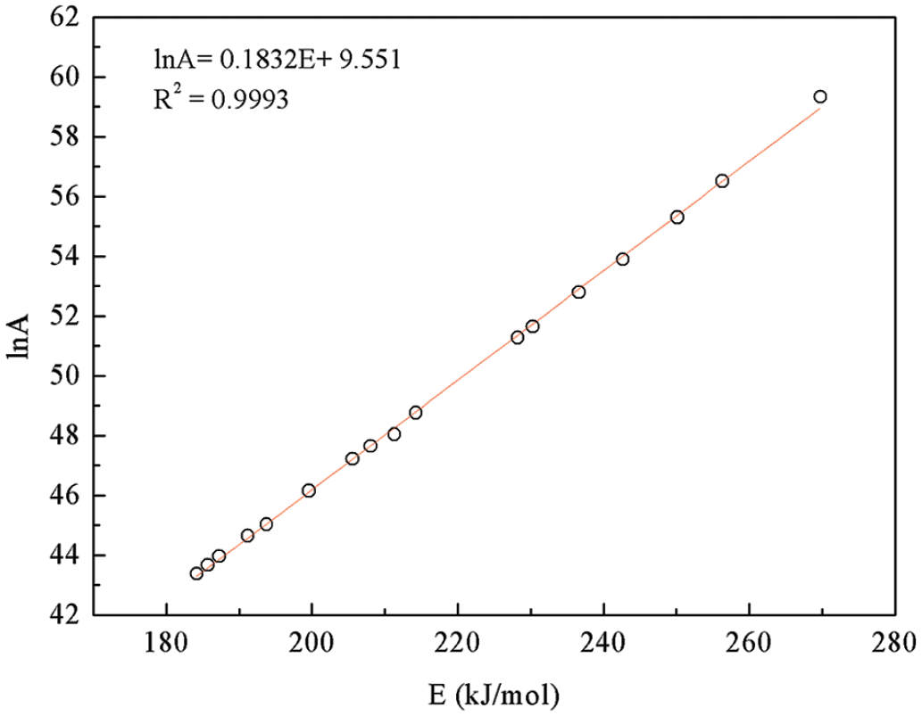
Compensation plot of lnA versus E.

Conclusions

In this work, a series of TG experiments was conducted to investigate the pyrolysis kinetics of plastic waste. The TG analysis revealed that the decomposition process can be divided into three stages with corresponding weight losses of 2.80–3.02%, 94.45–95.11% and 0.04–0.16%, respectively. The maximum peak temperatures were observed at 423, 433 and 439°C for three heating rates in the second stage. Based on the TG analysis, the activation energy and linear correlation coefficient were determined at different conversion rates using four model-free methods. The kinetic parameters calculated using the Friedman method displayed a similar trend to those determined by the KAS method. The same profiles were also observed for the FWO and Starink methods. However, the E_α and R² values determined from the Friedman and KAS methods fluctuated significantly. As a comparison, higher R² values were derived from the FWO method, which was the most reliable method used for the study of the reaction mechanism. Out of the CR methods, the F1 model gave higher R² values and the calculated E values were comparable to the average values from the FWO method. The value of lnA was calculated based on the F1 model and the FWO method and fell into the range 59.34–48.05 with α increasing from 0.1 to 0.9. Study of the kinetic compensation effect indicated that a compensation effect existed between the apparent activation energy and the pre-exponential factor during the pyrolysis of plastic waste.

Footnotes

Funding

The authors disclosed receipt of the following financial support for the research, authorship, and/or publication of this article: This work was financially supported by the Zhejiang Provincial Natural Science Foundation of China (Grant no. LY19B070008) and the National Natural Science Foundation of China (Grant no. 51911530460 and 51606055).

Declaration of conflicting interests

The authors declared no potential conflicts of interest with respect to the research, authorship, and/or publication of this article.

ORCID iD

Zhitong Yao

References

Aboulkas

El Bouadili

(2010) Thermal degradation behaviors of polyethylene and polypropylene. Part I: Pyrolysis kinetics and mechanisms. Energy Conversion and Management 51: 1363–1369.

Aguado

Serrano

Escola

(2008) Fuels from waste plastics by thermal and catalytic processes: a review. Industrial & Engineering Chemistry Research 47: 7982–7992.

Akahira

Sunose

(1971) Method of determining activation deterioration constant of electrical insulating materials. Research Report Chiba Institute of Technology (Science Technology) 16: 22–31.

Ashraf

Sattar

Munir

(2019) A comparative applicability study of model-fitting and model-free kinetic analysis approaches to non-isothermal pyrolysis of coal and agricultural residues. Fuel 240: 326–333.

Bach

Chen

(2017) Pyrolysis characteristics and kinetics of microalgae via thermogravimetric analysis (TGA): A state-of-the-art review. Bioresource Technology 246: 88–100.

Balart

Sánchez

López

, et al. (2006) Kinetic analysis of thermal degradation of recycled polycarbonate/acrylonitrile–butadiene–styrene mixtures from waste electric and electronic equipment. Polymer Degradation and Stability 91: 527–534.

Çepelioğullar

Haykırı-Açma

Yaman

(2016) Kinetic modelling of RDF pyrolysis: Model-fitting and model-free approaches. Waste Management 48: 275–284.

Cheng

Qiao

Huang

, et al. (2019) Effects of Ca and Na acetates on nitrogen transformation during sewage sludge pyrolysis. Proceedings of the Combustion Institute 37: 2715–2722.

Chong

Thangalazhy-Gopakumar

Gan

, et al. (2017) Kinetics and mechanisms for copyrolysis of palm empty fruit bunch fiber (EFBF) with palm oil mill effluent (POME) sludge. Energy & Fuels 31: 8217–8227.

10.

Coats

Redfern

(1964) Kinetic parameters from thermogravimetric data. Nature 201: 68.

11.

Cortés

Bridgwater

(2015) Kinetic study of the pyrolysis of miscanthus and its acid hydrolysis residue by thermogravimetric analysis. Fuel Processing Technology 138: 184–193.

12.

Datta

Kopczyńska

(2016) From polymer waste to potential main industrial products: Actual state of recycling and recovering. Critical Reviews in Environmental Science and Technology 46: 905–946.

13.

Deng

, et al. (2017) Emission characteristics of PBDEs during flame-retardant plastics extruding process: field investigation and laboratorial simulation. Environmental Science and Pollution Research 24: 22450–22457.

14.

Ding

Ezekoye

, et al. (2017) Comparative pyrolysis behaviors and reaction mechanisms of hardwood and softwood. Energy Conversion and Management 132: 102–109.

15.

Dou

Park

Lim

, et al. (2007) Pyrolysis characteristics of refuse derived fuel in a pilot-scale unit. Energy & Fuels 21: 3730–3734.

16.

Doyle

(1965) Series approximations to the equation of thermogravimetric data. Nature 207: 290.

17.

Flynn

Wall

(1966) A quick, direct method for the determination of activation energy from thermogravimetric data. Journal of Polymer Science Part B: Polymer Letters 4: 323–328.

18.

Friedman

(1964) Kinetics of thermal degradation of char-forming plastics from thermogravimetry. Application to a phenolic plastic. Journal of Polymer Science Part C: Polymer Symposia 6(1): 183–195.

19.

Geyer

Jambeck

Law

(2017) Production, use, and fate of all plastics ever made. Science Advances 3: e1700782.

20.

Hamad

Kaseem

Deri

(2013) Recycling of waste from polymer materials: An overview of the recent works. Polymer Degradation and Stability 98: 2801–2812.

21.

Hardi

Imai

Theppitak

, et al. (2018) Gasification of char derived from catalytic hydrothermal liquefaction of pine sawdust under a CO₂ atmosphere. Energy & Fuels 32: 5999–6007.

22.

Jung

Kim

(2013) The influence of reaction parameters on characteristics of pyrolysis oils from waste high impact polystyrene and acrylonitrile–butadiene–styrene using a fluidized bed reactor. Fuel Processing Technology 116: 123–129.

23.

Khawam

Flanagan

(2005) Complementary use of model-free and modelistic methods in the analysis of solid-state kinetics. The Journal of Physical Chemistry B 109: 10073–10080.

24.

Khawam

Flanagan

(2006) Solid-state kinetic models: basics and mathematical fundamentals. The Journal of Physical Chemistry B 110: 17315–17328.

25.

Kissinger

(1956) Variation of peak temperature with heating rate in differential thermal analysis. Journal of Research of the National Bureau of Standards 57: 217–221.

26.

Deng

(2014) Occurrence, characteristics and leakage of polybrominated diphenyl ethers in leachate from municipal solid waste landfills in China. Environmental Pollution 184: 94–100.

27.

Liu

Liao

(2017) Thermal behavior of vehicle plastic blends contained acrylonitrile-butadiene-styrene (ABS) in pyrolysis using TG-FTIR. Waste Management 61: 315–326.

28.

Pang

(2015) Mechanism study on char formation of zinc acetylacetonate on ABS resin. Chinese Journal of Polymer Science 33: 772–782.

29.

Wang

Yang

, et al. (2018) Comparison of the thermal degradation behaviors and kinetics of palm oil waste under nitrogen and air atmosphere in TGA-FTIR with a complementary use of model-free and model-fitting approaches. Journal of Analytical and Applied Pyrolysis 134: 12–24.

30.

Ozawa

(1965) A new method of analyzing thermogravimetric data. Bulletin of the Chemical Society of Japan 38: 1881–1886.

31.

Özveren

Özdoğan

(2013) Investigation of the slow pyrolysis kinetics of olive oil pomace using thermo-gravimetric analysis coupled with mass spectrometry. Biomass and Bioenergy 58: 168–179.

32.

Papari

Hawboldt

(2015) A review on the pyrolysis of woody biomass to bio-oil: Focus on kinetic models. Renewable and Sustainable Energy Reviews 52: 1580–1595.

33.

Pérez

Teixeira

Rincón

, et al. (2012) Understanding the crystallization mechanism of a wollastonite base glass using isoconversional, IKP methods and master plots. Journal of the American Ceramic Society 95: 3441–3447.

34.

Polli

Pontes

Araujo

, et al. (2009) Degradation behavior and kinetic study of ABS polymer. Journal of Thermal Analysis and Calorimetry 95: 131–134.

35.

Liu

, et al. (2019) An efficient magnetic carbon-based solid acid treatment for corncob saccharification with high selectivity for xylose and enhanced enzymatic digestibility. Green Chemistry 21: 1292–1304.

36.

Rahimi

García

(2017) Chemical recycling of waste plastics for new materials production. Nature Reviews Chemistry 1: 0046.

37.

Sharuddin

SDA

Abnisa

Daud

WMAW

, et al. (2016) A review on pyrolysis of plastic wastes. Energy Conversion and Management 115: 308–326.

38.

Sokoto

Bhaskar

(2018) Pyrolysis of Waste Castor Seed Cake: A Thermo-Kinetics Study. European Journal of Sustainable Development Research 2: 18.

39.

Song

Liu

(2016) Pyrolysis characteristics and kinetics of low rank coals by distributed activation energy model. Energy Conversion and Management 126: 1037–1046.

40.

Srivastava

Chandel

Mehta

(2017) Calorimetric studies of crystallization for multi-component glasses of Se-Te-Sn-Ag (STSA) system using model-free and model-fitting non-isothermal methods. Journal of Thermal Analysis and Calorimetry 128: 907–914.

41.

Suzuki

Wilkie

(1995) The thermal degradation of acrylonitrile-butadiene-styrene terpolymei as studied by TGA/FTIR. Polymer Degradation and Stability 47: 217–221.

42.

Szabo

Olah

Ronkay

, et al. (2011) Characterization of the liquid product recovered through pyrolysis of PMMA-ABS waste. Journal of Analytical and Applied Pyrolysis 92: 19–24.

43.

Tanaka

(2005) The theory and practice of thermoanalytical kinetics of solid-state reactions. Journal of Thermal Analysis and Calorimetry 80: 795–797.

44.

Vyazovkin

Burnham

Criado

, et al. (2011) ICTAC Kinetics Committee recommendations for performing kinetic computations on thermal analysis data. Thermochimica Acta, 520: 1–19.

45.

Wang

Zhang

Liu

, et al. (2012) Pyrolysis and combustion characteristics of coals in oxyfuel combustion. Applied Energy 97: 264–273.

46.

Zhou

(2018) Reaction mechanism, cure behavior and properties of a multifunctional epoxy resin, TGDDM, with latent curing agent dicyandiamide. RSC Advances 8: 8248–8258.

47.

Yang

Rafael Castilleja

Barrera

, et al. (2004) Thermal analysis of an acrylonitrile–butadiene–styrene/SWNT composite. Polymer Degradation and Stability 83: 383–388.

48.

Yao

, et al. (2019a) Kinetic modeling study on the combustion treatment of cathode from spent lithium-ion batteries. Waste Management & Research 38(1): 100–106.

49.

Yao

, et al. (2019b) Comparative study on the pyrolysis kinetics of polyurethane foam from waste refrigerators. Waste Management & Research. Epub ahead of print 10 October 2019. DOI: 10.1177/0734242X19877682.

50.

, et al. (2019) Thermal treatment of flame retardant plastics: A case study on a waste TV plastic shell sample. Science of The Total Environment 675: 651–657.

51.

Yuan

Cao

, et al. (2017) Cattle manure pyrolysis process: Kinetic and thermodynamic analysis with isoconversional methods. Renewable Energy 107: 489–496.

52.

Zhu

Feng

, et al. (2015) Kinetics of pyrolysis of ramie fabric wastes from thermogravimetric data. Journal of Thermal Analysis and Calorimetry 119: 651–657.