A periodic micromechanical model for the rate- and temperature-dependent behavior of unidirectional carbon fiber-reinforced PVDF

Abstract

The rate- and temperature-dependent mechanical behavior of unidirectional carbon fiber-reinforced polyvinylidene fluoride (PVDF) is investigated through uniaxial tension and compression experiments under various off-axis loading conditions. To improve the understanding of the behavior of the composite, a 3D micromechanical model is developed. Microscopic analyses are used to characterize the geometrical properties of the UD composite at the fiber length-scale. These properties are used to construct a periodic 3D representative volume element (RVE). In combination with periodic boundary conditions, uniaxial macroscopic deformation (in any possible direction) is applied to the RVE to accurately and efficiently model off-axis loading. The rate- and temperature-dependent behavior of the PVDF matrix is accurately described using an elasto-viscoplastic constitutive model. The finite element simulations of uniaxial tension and compression tests are compared to the experimental data and the micromechanical response is analyzed. The micromechanical model accurately describes the rate-dependent macroscopic behavior of unidirectional carbon fiber-reinforced PVDF for various off-axis loading directions at different temperatures. Analysis of the local matrix response in the RVE reveals the influence of the matrix on the macroscopic behavior of the composite.

Introduction

The global transition from fossil fuels to renewable energy sources has sparked an increased interest in hydrogen as a clean and versatile energy carrier. Renewable energy sources, such as wind and solar, have emerged as viable options for producing hydrogen through electrolysis. ¹ Considering the off-shore production of green hydrogen, the need for efficient transport and storage facilities becomes imperative. The materials used for these facilities must be able to withstand the tough off-shore conditions, such as low temperatures, high mechanical loads, and saltwater exposure. Thermoplastic composite pipes are a potential solution for the safe, reliable, and sustainable transport of green hydrogen. The structural integrity of these multi-layered pipes is governed by a fiber-reinforced thermoplastic composite layer. In particular, carbon fiber-reinforced polyvinylidene fluoride (PVDF) is proposed as a favorable combination for the reinforcement layer, because of its low specific density, high strength and stiffness, excellent thermal properties and chemical resistance and good gas barrier properties.^2–4 Furthermore, compared to conventional steel, fiber-reinforced thermoplastic composites are not susceptible to corrosion, which is a substantial benefit in an off-shore environment. For a safe and reliable use of carbon fiber-reinforced PVDF, its thermo-mechanical behavior must be well understood.

Over the past years, the interest in carbon fiber-reinforced PVDF and its applications has been steadily growing, leading to several experimental studies into its material behavior. Some studies investigated the potential of using PVDF by exploiting its piezoelectric properties to enable integrated structural health monitoring of carbon fiber-reinforced PVDF composites.^5,6 Others investigated the effect of the addition of short carbon fibers to enhance the wear resistance of carbon fiber-reinforced PVDF composites.^7,8 Some studies characterized and made an effort to improve the adhesion between PVDF and short carbon fibers^9–11 as well as unidirectional (UD) carbon fibers.^12–15 However, to the best of the authors’ knowledge, no experimental studies into the rate- or temperature-dependent behavior of UD carbon fiber-reinforced PVDF subjected to various complex loading conditions have been reported.

Compared to the extensive experimental efforts, only few studies exploit a modeling framework to analyze or predict the behavior of carbon fiber-reinforced PVDF. Odegard ¹⁶ used a mean-field approach to predict the macroscopic electro-mechanical properties of piezoelectric polymer composites, amongst which carbon fiber-reinforced PVDF was one of the studied materials. Greminger et al. ¹⁷ proposed a multiscale finite element model to predict the electro-mechanical performance of plain weave carbon fiber-reinforced PVDF. Both studies focus on the electro-mechanical properties of the composite in the elastic regime. For a complete understanding of the intrinsic behavior of the composite, the nonlinear and rate- and temperature-dependent nature of the material must be taken into account.

Despite previous studies, the mechanical behavior of unidirectional carbon fiber-reinforced PVDF has not been explored thoroughly, both from an experimental and a numerical point of view. To address the latter, a more widely used technique enabling an in-depth numerical analysis of the micromechanical behavior of fiber-reinforced polymers is used; computational micromechanics. ¹⁸ A widespread technique is the use of a representative volume element (RVE) to extract the homogenized macroscopic behavior, based on the underlying microstructure of the material. There are several definitions for an RVE, mostly determined by the purpose of the RVE. ¹⁹ Under the requirement that the RVE should be a statistical representation of the actual microstructure, the corresponding dimensions may be significant, ²⁰ especially if the microstructure reveals an irregular distribution of constituents. The RVE may also be defined such that it sufficiently accurately describes the desired macroscopic quantities, using the smallest possible dimensions. This, however, depends not only on the behavior of the microscale constituents, but also on the desired macroscopic quantities, in particular if one wants to address the initiation and propagation of damage. ²¹ The determination of the size of the RVE will therefore be a trade-off between the statistical representativeness and the accuracy of the model on the one hand, and computational cost on the other hand. For UD fiber-reinforced polymers, not only the size of the RVE matters, but also the distribution of fibers inside the RVE. Trias et al. ²² compared the micromechanical response of models with periodic and random fiber distributions. They concluded that periodic distributions can be used to predict some effective properties, but fail to accurately predict failure initiation or propagation. A similar conclusion was drawn by Ghayoor et al. ²³ Furthermore, Ghayoor and co-workers showed that stress concentrations in the matrix are governed by the fiber volume fraction, randomness of the fiber distribution, and minimum inter-fiber distance. To incorporate all these aspects in this study, the RVE geometry is based on microscopic images of a cross section of the UD composite. This enables a reliable description of the microstructure in the model.

Besides the proper definition of the microstructure, the intrinsic behavior of the constituents is an equally important aspect of the model. The PVDF matrix is a semi-crystalline thermoplastic polymer that exhibits rate- and temperature-dependent behavior. An experimental study into the intrinsic behavior of neat PVDF was performed by Pini et al. ²⁴ Uniaxial tension and compression experiments were performed at different strain rates and temperatures to investigate the influence of processing conditions on the yield kinetics. The results revealed a highly nonlinear behavior of PVDF. The influence of loading conditions on the matrix behavior will therefore also have an impact on the response of the composite, especially when the major fraction of the applied mechanical load is carried by the PVDF matrix. To accurately describe the rate- and temperature-dependent intrinsic behavior of the PVDF matrix, the elasto-viscoplastic constitutive model described in a previous work will be used. ²⁵ The constitutive model is used to predict the short- and long-term rate-dependent behavior of PVDF at temperatures 23, 55, and 75°C. All testing temperatures are well within the range of the glass transition temperature, T_g = −35°C and the melting temperature, T_m = 165°C.

In engineering applications, UD fiber-reinforced polymers are generally stacked in layups with alternating fiber orientations. The orientation of the anisotropic fibers has an important influence on the mechanical behavior of the composite. Yet, many numerical studies on UD fiber-reinforced polymers only address the transverse response. Unfortunately, describing the off-axis behavior of UD fiber-reinforced polymers in FE-models requires large dimensions in the longitudinal fiber direction. Fallahi et al. proposed a rather simple but effective constitutive model to describe the off-axis loading-unloading behavior of UD fiber-reinforced composites. ²⁶ This model however does not give any information about the response at the microscale. Taheri-Behrooz et al. proposed a 3D RVE model of a single fiber embedded in an epoxy matrix to analyze the mechanical properties of a UD fiber-reinforced composite. ²⁷ They used periodic boundary conditions to apply different macroscopic deformations on the RVE, but this does not allow for uniaxial loading conditions. In a study by Zhu et al. ²⁸ a micromechanical model is used to describe the behavior of fiber-reinforced PEEK under off-axis tensile loading. The micromechanical model was based on a periodic stacking of fibers and therefore did not incorporate any variation of the fiber distribution in the composite. Zhou et al. ²⁹ studied the off-axis compressive behavior of glass fiber-reinforced polymers, but only a limited number of fibers were included in the FE-model because of the large dimensions in the fiber direction. Furthermore, different models were required for different off-axis loading angles. Sun et al. ³⁰ performed a numerical study into the behavior of UD carbon fiber-reinforced epoxy under different loading conditions, where uniform traction or displacement boundary conditions were applied to the RVE. However, the use of uniform boundary conditions requires a larger RVE, especially in the fiber direction, compared to periodic boundary conditions. ³¹ In a recent study by Kovačević et al. a strain-rate-based arc-length method is used to perform simulations on UD carbon fiber-reinforced PEEK under off-axis uniaxial loading conditions in combination with periodic boundary conditions. ³² This algorithm requires the additional implementation of the solution procedure, which is at the expanse of its versatility.

To obtain a profound understanding of the mechanical behavior of carbon fiber-reinforced PVDF, the rate- and temperature-dependent behavior of UD carbon fiber-reinforced PVDF under off-axis loading is here investigated, both experimentally and numerically. The experimental component of this work consists of uniaxial tension and compression experiments that are performed at different strain rates and temperatures on UD samples with varying fiber orientations. For the numerical part, a similar approach as described by Kovačević et al. ³² is used here, although the present framework differs on several points. A micromechanical model is developed that describes the mechanical behavior of UD carbon fiber-reinforced PVDF. A periodic 3D RVE is defined that accurately represents the microstructure of the composite. The constitutive behavior of the matrix is described by the elasto-viscoplastic constitutive model described in Ref. 25. Finally, periodic boundary conditions are applied to the 3D RVE. To simulate uniaxial loads under an arbitrary angle with respect to the fiber orientation, the algorithm developed by Van Nuland et al. ³³ is used. Van Nuland and co-workers used this algorithm to apply periodic boundary conditions on a 2D microscale RVE in combination with uniaxial macroscopic loading in an arbitrary direction and extended the method to 3D in Ref. 34. The strength of this algorithm is that only a small out-of-plane thickness of the 3D micromechanical RVE is required to capture the anisotropic macroscopic behavior. The macroscopic deformation can be applied in any direction without altering the dimensions of the RVE. Furthermore, the finite element implementation of the algorithm only entails linear tying relations between nodal DOFs, which is facilitated in most FE-packages, without the requirement for an additional solution algorithm. The constructed micromechanical model is then used to perform FE-simulations of uniaxial compression and tension tests for various off-axis loading directions at different constant applied strain rates, after which the results are compared with the experiments. The micromechanical model is also used to study the influence of the loading conditions on the local response of the matrix. Both simulations and experiments are performed at three different temperatures, that is, 23, 55, and 75°C.

The paper is organized as follows. First, the sample preparation and experimental methods and results are described, followed by the definition of the micromechanical model. Subsequently, the results from the simulations are analyzed and compared to experiments. Finally, the main conclusions are presented.

Throughout this paper, scalar variables are denoted as a or A, and second-order tensors are denoted as A. Together with the Einstein summation convention, the dyadic product between two vectors is defined as $\overrightarrow{a}\overrightarrow{b}=a_i{b}_j{\overrightarrow{e}}_i{\overrightarrow{e}}_j$ , the dot product is defined as $\mathbf{A}·\overrightarrow{b}=A_{ij}{b}_j{\overrightarrow{e}}_i$ , and the cross product is defined as $\overrightarrow{a}\times \overrightarrow{b}$ . Here $\left\{{\overrightarrow{e}}_1,{\overrightarrow{e}}_2,{\overrightarrow{e}}_3\right\}$ is the Cartesian vector basis.

Experiments

Material and specimen preparation

Prepreg carbon fiber-reinforced PVDF tape, Evolite^® F3050, was kindly provided by Solvay Composite Materials (Harve de Grace, Maryland, USA) in the form of unidirectional tape. The tape thickness was 0.25 mm, and the fiber content was 50% in weight. The tape was cut with a guillotine cutter into pieces. In order to obtain laminates, the pieces were stacked into a picture frame mold measuring 200 × 200 mm². The mold was prepared with a releasing agent. In addition, a Kapton film was used to prevent adhesion between the laminates and the mold itself. Once the mold was filled and closed, it was put in the hot press at 210°C and kept at that temperature for 90 min to ensure thermal equilibrium. Next, a pressure up to 7 bars was applied in steps to force the trapped air to escape, with approximately 1 min of hold time between steps. After 30 min, the mold was cooled down at a cooling rate of 10°C/min. The whole process was carried out under vacuum.

Laminates of different thicknesses and different fiber orientations were prepared, whereby the plates were demolded, trimmed, and cut with a diamond blade circular saw. In order to obtain plates with different fiber orientations, the tape was cut at different angles, and then the pieces were loosely welded together with a soldering iron in order to handle them and place them in the mold. In the stacking sequence, adjacent plies were overlapped to avoid alignment of the weld lines. A different number of plies were used to obtain laminates of different thicknesses.

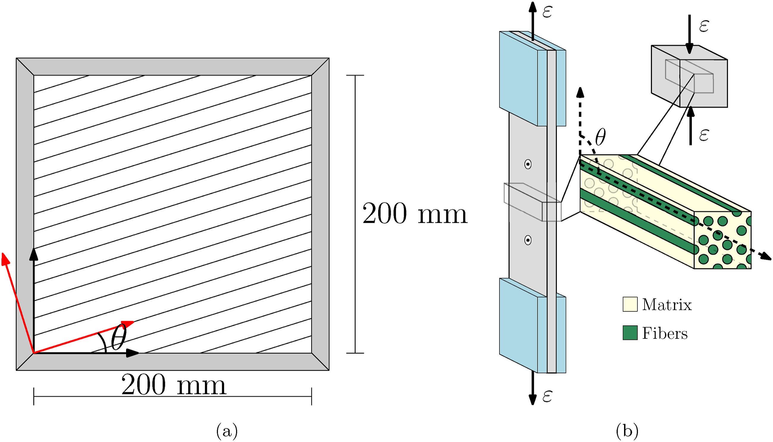
A detailed description of the preparation of the different types of specimens is given below.

• Tensile Specimens: In this case, specimens of 1 and 1.5 mm thickness were prepared by placing 4 and 6 layers of tape in the mold, respectively. The laminates were prepared with fibers oriented at θ = 10°, 20°, 30°, 45°, 60°, and 90° with respect to the mold reference system (see Figure 1(a)). The plates were then cut with the diamond blade saw into strips of 200 × 20 mm² for the angles 30°, 45°, 60°, and 90°. In the case of fiber orientations θ = 10° and 20°, a width of 10 mm was adopted. The thickness of the 10°, 20°, and 30° specimens was 1 mm and for the angles of 45°, 60°, and 90°, 1.5 mm thick specimens were prepared as well to verify that the results are independent of sample thickness. See Figure 1(b) for the fiber alignment in the specimen with respect to the uniaxial loading direction in terms of the angle θ. Tabs were machined from a ± 45° fiber glass/epoxy plate. Prisms of 50 × 20 × 1 mm³ and 50 × 10 × 1 mm³ were obtained. The tabs were then glued to the specimens with a CA glue and left overnight to cure (see the light blue prisms in Figure 1(b)). Adhesive markers were placed along the center line of the specimens at a separating distance of approximately 50 mm.

• Compression Specimens: Plates of 6 mm thickness were prepared by placing 24 plies of tape into the mold. Plates with a fiber orientation of 45° and 90° were cut into prisms with a cross section of 6 × 6 mm² with the diamond blade saw. The prisms were then taped together and cut transversally in order to obtain cubic samples (6 × 6 × 6 mm³) with fiber orientation of θ = 0°, 45°, and 90°. See Figure 1(b) for the fiber alignment in the specimen with respect to the uniaxial loading direction.

• Microscopic fiber distribution analysis: A plate of 2.5 mm thickness was prepared by placing 10 plies of tape into the mold ensuring a fiber orientation of 90° with respect to the mold reference frame. A sample of 14 mm in width was cut from the plate with the diamond blade saw. To prepare the sample for microscopic analysis, it was embedded in an epoxy resin. After the epoxy was cured, the surface was polished in 5 steps. In the first three steps, a grinding paper of 1000, 2000, and 4000 grade in a water suspension was used, followed by a diamond suspension and a colloidal silica suspension in steps 4 and 5, respectively.

Figure 1.

(a) Schematic representation of the tape placed inside the picture frame mold where the fibers are oriented under an angle θ with respect to the bottom edge of the mold. (b) Schematic representation of the tensile and compression samples where the applied deformation ɛ is oriented in the vertical direction. The orientation of the fibers with respect to the uniaxial loading direction is indicated by the angle θ. The dimensions are not to scale.

Tests facilities

Microscopy analysis

The microscopic analysis was performed using a Keyence VHX-7000 optical microscope. The complete image of the sample was captured by stitching the partial microscopic scans at 400x magnification.

Mechanical testing

Uniaxial tensile tests were carried out on a Zwick Z010 universal tester, equipped with a 10 kN load cell and a thermal chamber. A laser level was used to ensure alignment between the specimen and the load line. Tests were performed at constant engineering strain rates between 10⁻⁶ and 10⁻² s⁻¹ at temperatures of 23, 55, and 75°C. Deformations were measured using an optical extensometer (Zwick videoXtens). The engineering strain was computed from the displacement between the gauge points. The engineering stress was calculated from the initial cross section of the specimen. Tests were carried out until failure of the specimens.

Uniaxial compression tests were performed on a Zwick 1473 universal tester, equipped with a 100 kN load cell and a temperature chamber. Tests were carried out at constant engineering strain rates varying from 10⁻⁵ to 10⁻¹ s⁻¹ at temperatures of 23, 55, and 75°C. In order to avoid friction between the specimen and the compression plates, dry PTFE spray was used for lubrication.

For fiber orientations larger than 0°, the raw displacement data of each test was corrected for the compliance of the test setup and the machine. This compliance was measured by performing a compression test without a sample. For the compression tests with a fiber orientation of 0°, the displacement of the compression plates was tracked optically by placing adhesive markers. This solution proved to be necessary as the stiffness of the specimen was larger than that of the machine, resulting in inaccurate corrections. For all cases, the engineering strain was calculated from the displacement between the compression plates. The engineering stress was calculated using the initial cross-sectional area of the specimen.

For all tests where the temperature was different from the room temperature, the specimens were climatized in the thermal chamber for 10 min to reach thermal equilibrium.

Results

Microscopy analysis

The image of the cross section obtained with optical microscopy is shown in Figure 2(a) , and a thin slice that spans the full height of the sample is shown in Figure 2(b). The stacking of the unidirectional plies is indicated by the yellow arrows and can also be observed in the images from the matrix-rich bands perpendicular to the stacking direction. Three close-ups of 200 × 200 μm² of the scan reveal some interesting features of the fiber distribution in the sample (see Figure 2(c)-(e)). First, there is a non-uniform spatial fiber distribution as demonstrated by the matrix-rich regions in Figure 2(c) compared to the dense fiber packing in Figure 2(d). Second, Figure 2(e) shows a horizontal band with hardly any fibers, revealing the boundary between two stacked plies. These variations in spatial fiber distributions may have an influence on the macroscopic behavior of the composite. This is studied in more detail in the Section RVE generation where the microstructure is defined for the FE-simulations. Finally, a close-up of 62.5 × 62.5 μm² is shown in Figure 2(f) which highlights two fibers with irregular shapes. The dark spots in these fibers represent fiber breakage which is most likely caused by polishing of the specimen. Although fiber breakage was reduced to a minimum by optimizing the polishing procedure, it could not be avoided completely.

Figure 2.

(a) Micrograph of the full cross section and (b) a thin slice over the full height of the specimen and close-ups of (c–e) 200 × 200 μm² and (f) 62.5 × 62.5 μm² with different fiber distributions. The stacking direction of unidirectional plies is indicted by the yellow arrows in (a) and (b).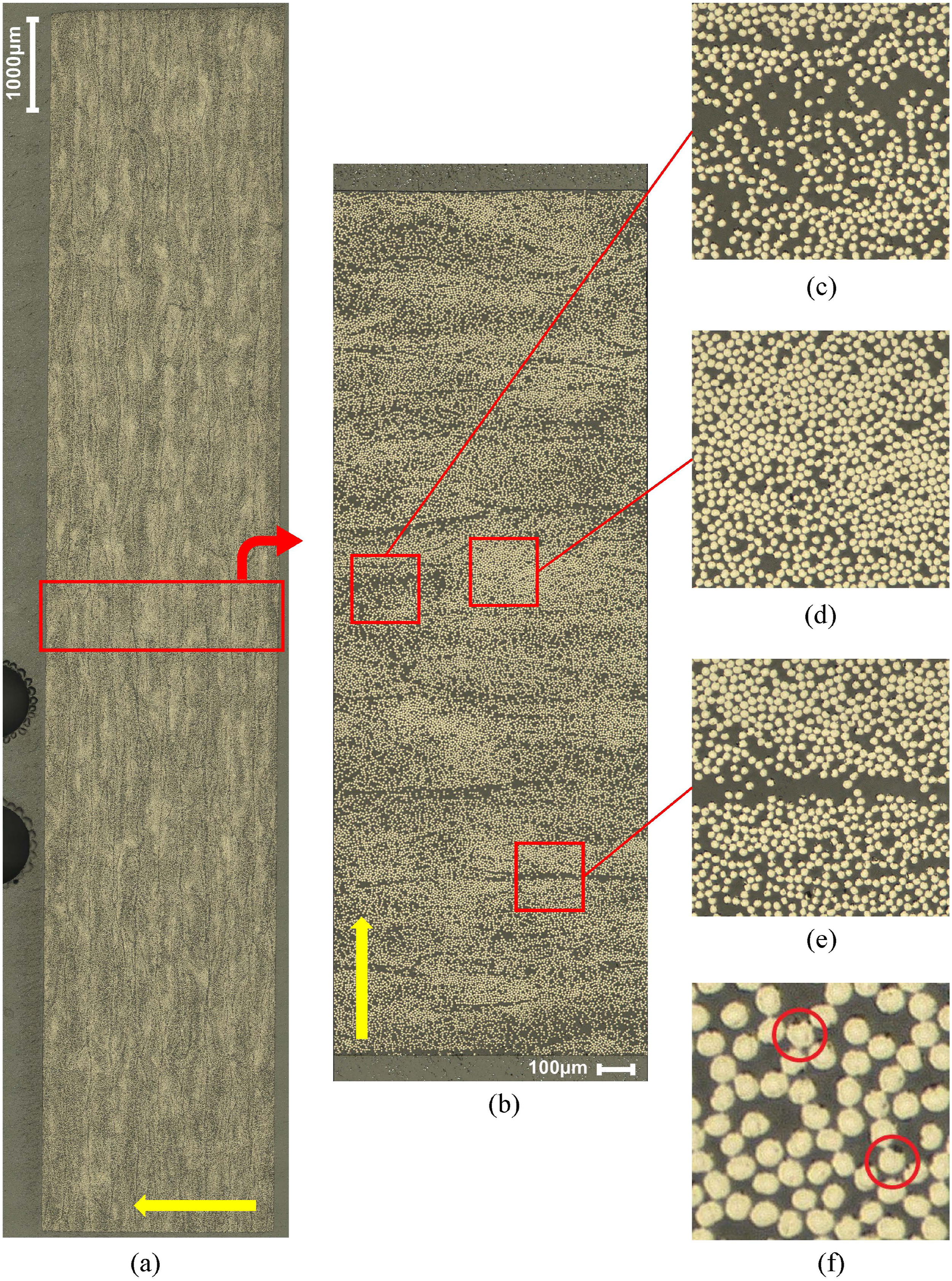

Uniaxial testing

The fractured specimens from the uniaxial tensile tests with different fiber orientations are shown in Figure 3. Note that the width of the specimens for θ = 10° and 20° is smaller than for the other fiber orientations. In all cases, the specimens failed along the fiber orientation.

Figure 3.

Fractured tensile specimens with different fiber orientations. The markers were used to measure the deformation of the specimens.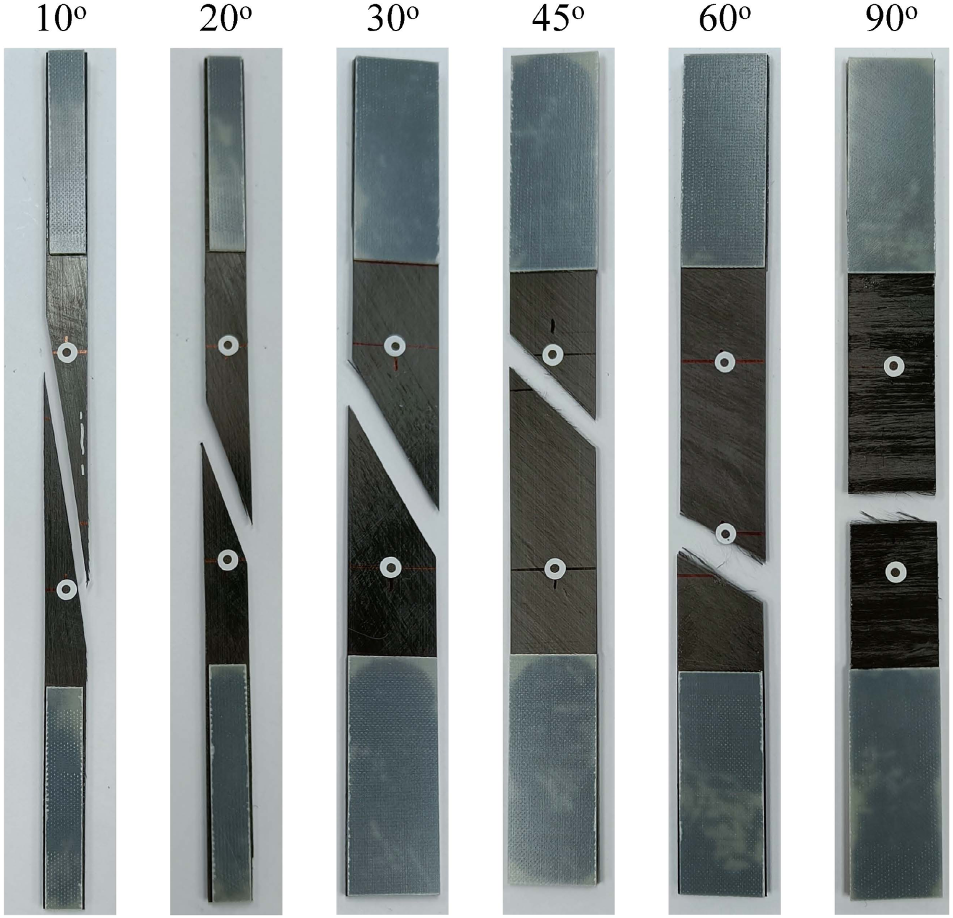

The engineering stress-engineering strain results of some uniaxial tensile and compression tests under different loading conditions are shown in Figure 4. The response of transverse tension and compression experiments at temperatures 23 and 75°C for varying constant strain rates is shown in Figure 4(a) and (b), respectively. All transverse tension experiments show brittle failure at small strain levels. This may indicate a weak adhesion between the fibers and the matrix, which is a known challenge for carbon fibers embedded in a PVDF matrix.^9,13 Furthermore, the variation of the applied strain rates does not result in large differences. However, the transverse compression results in Figure 4(b) clearly reveal the rate-dependent nature of the composite, which originates from the rate-dependent behavior of the PVDF matrix. After the peak in the compressive stress is reached, macroscopic cracks nucleate and the deformation of the compression samples is no longer homogeneous. Therefore, the engineering stress is not reliable beyond the stress peak, and the data is shown in gray.

Figure 4.

Uniaxial tension and compression results for different loading conditions. Transverse tension (a) and compression (b) at 23 and 75°C for different strain rates. (c) Transverse tension at temperatures 23, 55, and 75°C at 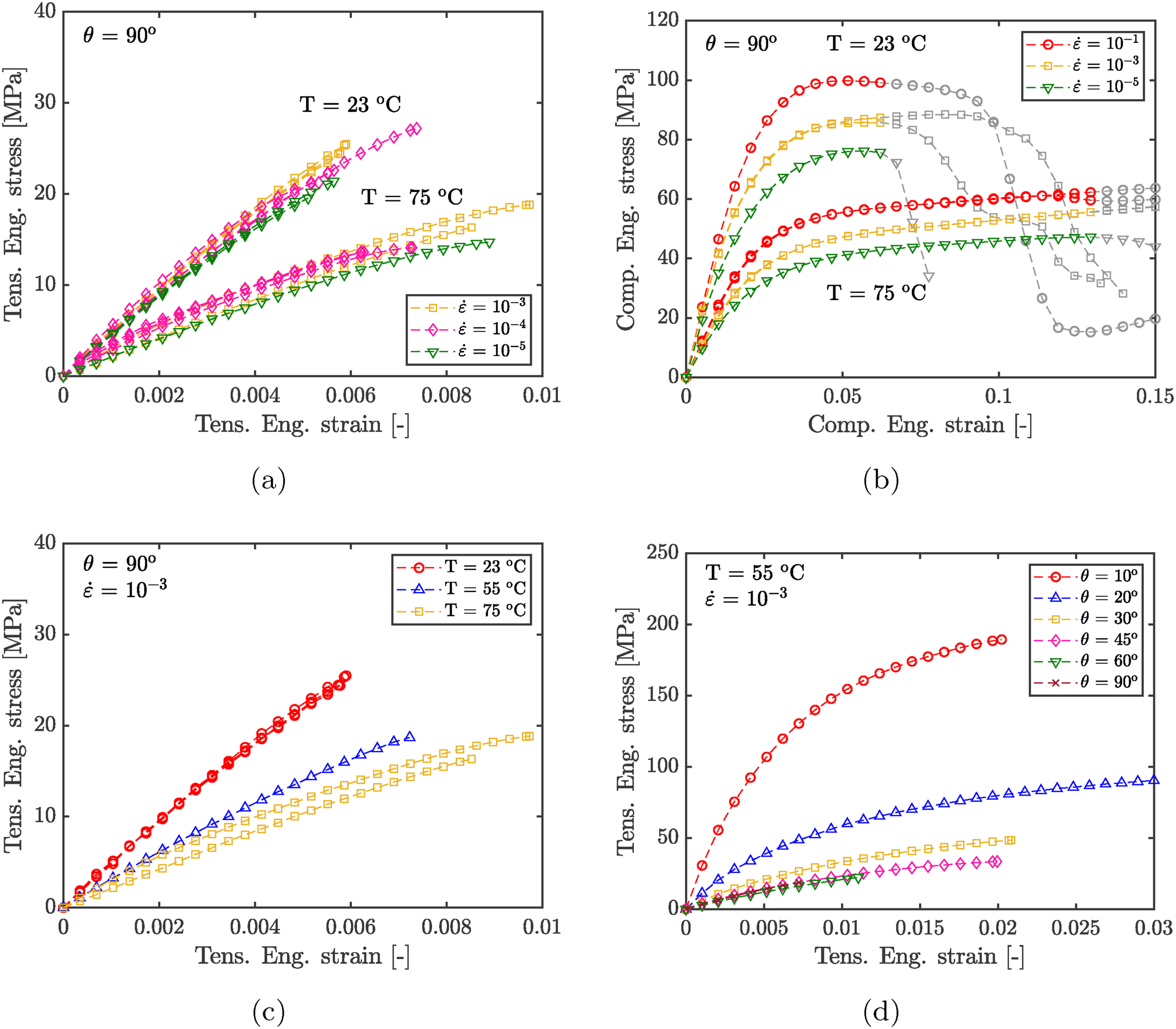$\stackrel{.}{\epsilon }={10}^{-3}{\mathrm{s}}^{-1}$ and (d) tension for varying fiber orientations θ at 55°C and $\stackrel{.}{\epsilon }={10}^{-3}{\mathrm{s}}^{-1}$ .

The transverse tensile response at three temperatures 23, 55, and 75°C at a strain rate of 10⁻³ s⁻¹ is shown in Figure 4(c). With increasing temperature, the stiffness and the transverse tensile strength of the composite decrease, whereas the strain at failure increases. The latter suggests increased plastic deformations in the matrix.

The tensile response of the composite at 55°C and a strain rate of 10⁻³ s⁻¹ for different fiber orientations are shown in Figure 4(d). Obviously, the tensile strength of the composite increases with a decreasing fiber orientation θ, as the preferential direction of the fibers is more aligned with the direction of applied deformation. Also the strain at failure increases upon decrease of the fiber orientation θ.

Micromechanical model

The main components of the micromechanical model are presented in this section. First the procedure for the generation of a 3D RVE is discussed after which the application of periodic boundary conditions for uniaxial macroscopic loading along different directions is explained. Finally, a concise description of the constitutive models of the matrix and the fibers is given.

RVE generation

The dimensions of the RVE should be sufficiently large to capture the spatial microstructural variations in the UD composite in order to be representative. However, with increasing RVE dimensions, the required computational time increases as well. Hence, a trade-off must be found between statistical representativeness and computational cost. For this micromechanical FE-model, the RVE geometry is constructed from the microscopic scan shown in Figure 2(b), which has dimensions of approximately 930 × 2550 μm². This microstructure is referred to as the global scan.

Microstructural characteristics

As there is only data available of the fiber weight fraction in the composite, but no accurate data for the density, the global fiber volume fraction is calculated from the composite sample in Figure 2(b), by comparing the intensity of each pixel, I_px, to a threshold intensity I_th. All pixels with an intensity above the threshold are assigned to a fiber and the remaining pixels are assigned to the matrix. The average fiber volume fraction V_f,global is then defined as

$V_{\mathrm{f},\text{global}}=\frac{N_{\mathrm{f}}}{N_{\text{tot}}}$

(1)

where N_f and N_tot are the number of pixels assigned to the fiber and the total number of pixels in the image, respectively. To avoid edge effects, the analyzed area in Figure 2(b) is restricted to 50 μm above the bottom edge and 50 μm below the top edge of the composite. The threshold I_th is chosen as the average pixel intensity in the analyzed area. This results in a global fiber volume fraction of V_f,global = 0.42. Different measures for I_th were analyzed, but this did not reveal a significant influence on the global fiber volume fraction.

The close-ups of the cross section in Figure 2(c)-(e) demonstrate the inhomogeneous distribution of the fibers in the sample. Consequently, there is a spatial variation in local fiber volume fraction over the cross section. Therefore, the fiber volume fraction is also calculated locally by defining a smaller region of size a × a inside the global scan in Figure 2(b). This length a is referred to as stencil size. The local fiber volume fraction is again calculated using equation (1), where N_f and N_tot now correspond to the amount of pixels in the local scan window. The threshold I_th is not changed and is the average intensity of the global scan. The distribution of the local fiber volume fraction will be different for varying stencil size a, converging to the global fiber volume fraction when the size recovers the global scan. The local fiber volume fraction V_f,local is computed for varying stencil sizes a, while following the trajectory sketched in Figure 5(a). The red square represents the stencil and the black rectangle is the global scan, restricted to 50 μm above the bottom edge and 50 μm below the top edge of the composite. Subsequently, the mean and standard deviation of the local fiber volume fraction for each size a are computed.

Figure 5.

(a) Trajectory for calculating the local fiber volume fraction in the global scan. (b) Mean and standard deviation of the local fiber volume fraction. (c) The probability distribution of the local fiber volume fraction, both for varying stencil size a.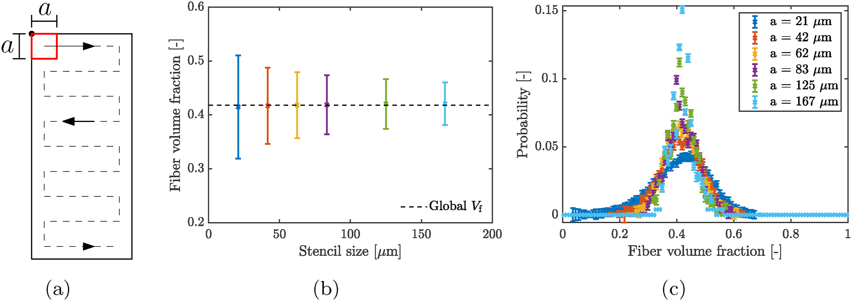

The result is shown in Figure 5(b). The dashed black line represents the global fiber volume fraction. The mean value of the local fiber volume fraction is hardly influenced by the stencil size, whereas the standard deviation decreases with increasing length a.

The probability distributions of the local fiber volume fraction for varying stencil size a are shown in Figure 5(c). The widest distribution is observed for the smallest stencil size, while the distribution becomes more narrow with increasing length a. For a stencil size a = 62.5 μm, the majority of the local fiber volume fractions are in a range between 0.3 and 0.5, but there are also closely packed regions with fiber fractions up to 0.65 or matrix-rich regions with fiber volume fractions as low as 0.25. Since the micromechanical model is used to predict the macroscopic behavior of the composite, the local fiber volume fraction must be equal to the global fiber volume fraction. From Figure 5(b), it is clear that the mean value of the local fiber volume fraction does not change for a ≥ 62.5 μm. Hence, the scan size 62.5 × 62.5 μm² is adopted for the generation of the RVE.

The standard deviation of the local fiber volume fraction for this stencil size is not yet constant for increasing stencil size a, which is also visible in the changing distributions in Figure 5(c). Three local snapshots with a stencil size of 62.5 × 62.5 μm² containing a different number of fibers are depicted in Figure 6, where only the scan in Figure 6(b) has an adequate fiber volume fraction, because it is close to the global fiber volume fraction. Furthermore, the fiber distribution over this scan is relatively homogeneous, that is, no significant fiber clustering is observed. Hence, this scan will be used for the generation of the RVE.

Figure 6.

Three scans with stencil size 62.5 × 62.5 μm² with fiber volume fractions (a) 0.24, (b) 0.42, and (c) 0.55.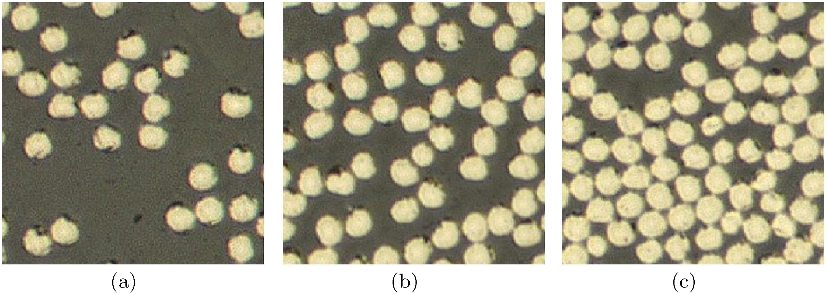

From scan to periodic RVE

To generate the RVE from the scan in Figure 6(b), the locations of the fibers are determined using the built-in MATLAB function imfindcircles. ³⁵ The number of detected fibers, n_f, in Figure 6(b) is equal to 55. The function imfindcircles does not result in an adequate measurement of the fiber radii. Therefore, two different options are analyzed. Option A is to calculate the average fiber radius, R_avg, according to

$n_{\mathrm{f}}\pi R_{\text{avg}}^2=V_{\mathrm{f}}{a}^2$

(2a)

$R_{\text{avg}}=a\sqrt{\frac{V_{\mathrm{f}}}{n_{\mathrm{f}}\pi }}$

(2b)

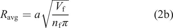
This results in an average fiber radius of 3.08 μm. Alternatively, option B is to count the number of pixels along the fiber diameter manually for each fiber in the scan and compute the average radius. In that case, the average fiber radius in Figure 6(b) equals 3.25 μm. Considering this average radius and the total number of 55 fibers, the fiber volume fraction of this single scan is equal to 0.47. The difference between the two methods can be explained by the irregularities in the fiber cross sections (black spots) caused by fiber damage during polishing, as explained before. To reduce the influence of fiber irregularities on the local fiber volume fraction, option B is adopted to compute the average fiber diameter and fiber volume fraction for scans with a = 62.5 μm at different locations in the global scan. This results in an average fiber radius of 3.25 μm and an average fiber volume fraction of 0.47. Therefore, a constant fiber radius of 3.25 μm is used in combination with the fiber locations determined from the scan in Figure 6(b).

The RVE that is used in the micromechanical FE analysis should be periodic. Furthermore, to ensure an adequate quality of the finite element discretization, a minimum separation between fibers is required. Consequently, the method described below is used to impose the required periodicity, while using the fiber locations from the microscopic scan in Figure 6(b) and a constant radius of 3.25 μm. It is based on a discrete element model (DEM) described in 36 where the fibers are considered as interacting circular particles.

1. Scaling: The domain of the scan is converted to unit dimensions and the fiber positions are scaled correspondingly. This unit domain is represented by the dashed black line in Figure 7(a) and the origin is defined at the left bottom corner. The fibers are placed in the domain at the scaled positions (red circles in Figure 7(a)).

2. Initialization: The initial size of the domain is increased to 1.1 × 1.1, without modifying the initial coordinates or size of the fibers with respect to the origin. This domain is represented by the black square in Figure 7(a). Then, for each fiber crossing the bottom or left boundary of the dashed domain, a ghost particle is added at the opposite boundary of the enlarged domain (the pink circles in Figure 7(a)). This step is essential for creating the required periodicity. After the initialization stage, the number of fibers in the domain remains constant. Note that fibers are allowed to overlap in the initial configuration, which may occur under the assumption of a constant fiber diameter.

3. Domain reduction: The domain size is reduced from the initial size 1.1 × 1.1 to the unit size 1.0 × 1.0 by shifting the right and top boundary inwards in small increments. At each increment, fibers outside the domain are moved inside by applying a vertical or horizontal shift equal to the current domain size. In the updated configuration, the overlapping fibers exert a repelling reaction force on each other, where the reaction force is linearly related to the overlap. Under the assumption of purely normal linear contact forces between each pair of intersecting fibers i and j, the reaction force and the corresponding acceleration, velocity, and displacement of the fibers are calculated. ³⁶ During the domain reduction, it is verified that the periodicity at the boundaries is maintained.

4. Equilibrium: When the domain reduction to unit size is complete, fibers may still be overlapping, resulting in repelling interaction forces and corresponding displacements. The addition of a dissipative term to the interaction forces, guarantees that the system eventually comes to an equilibrium (see Figure 7(b)). ³⁶ Consequently, the system in equilibrium will not have any overlapping fibers.

Figure 7.

(a) Initial fibers are drawn in dark red in the domain of size 1.1 × 1.1 and ghost fibers added in pink at the top and right boundary to ensure periodicity. (b) Reduced periodic domain of size 1.0 × 1.0 in equilibrium. (c) Difference between initial fiber positions in purple and fibers in the periodic equilibrium configuration in red.

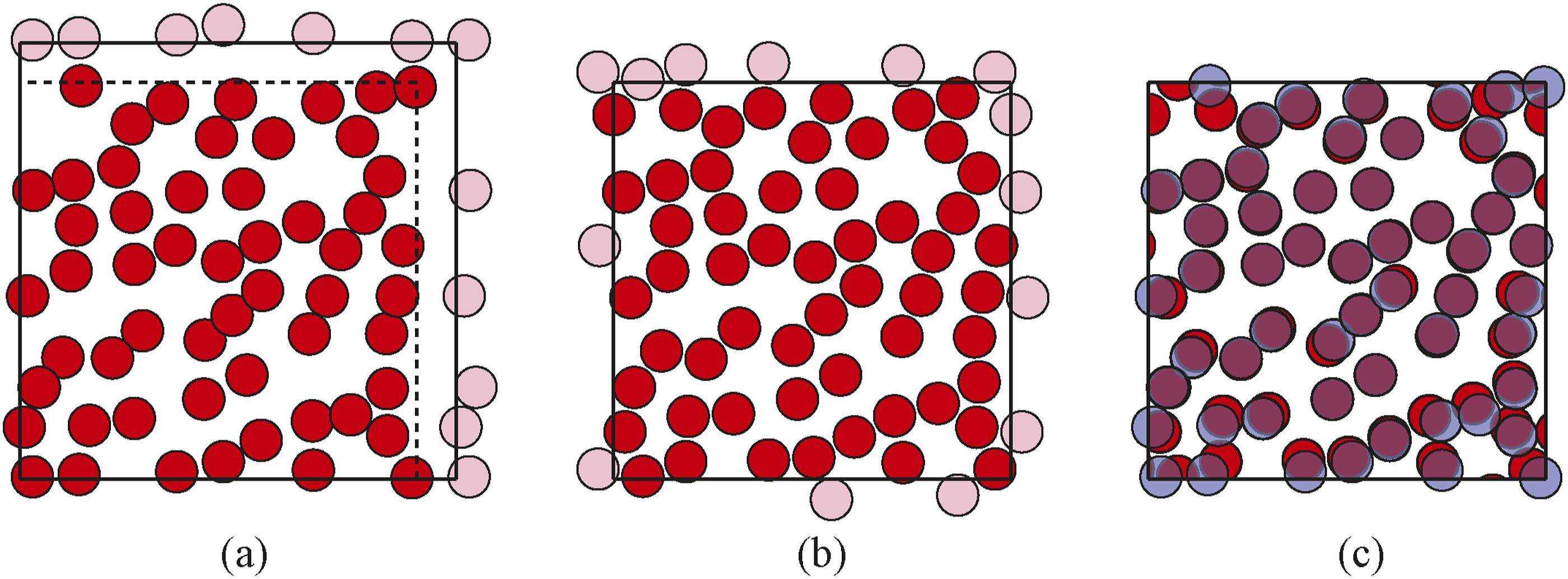
A minimum inter-fiber distance of 5% of the fiber diameter is used to ensure an adequate quality of the FE mesh, while reducing the displacements of the fibers with respect to the initial configuration to a minimum. Using this method, the initial fiber distribution obtained from the scan is preserved as much as possible. This results in a periodic geometry without overlapping fibers, in which the fiber distribution is close to the actual microstructure of the UD composite. This can be observed in Figure 7(c), where the difference between the initial fiber positions (purple) and the final fibers in the periodic equilibrium configuration (red) is shown. The figure also demonstrates that in the final configuration, no fibers are overlapping due to the constraint on the minimum inter-fiber distance. Note that the fiber volume fraction remains constant during the entire procedure, since no new fibers are added to the domain. That is, each fiber pair crossing the left/right or top/bottom boundary counts as a single fiber.

Finally, to obtain a 3D periodic RVE, the periodic 2D geometry that results from the procedure described above is simply extruded along the longitudinal fiber direction, automatically enforcing periodicity in the out-of-plane direction.

Uniaxial periodic boundary conditions

To enforce a macroscopically uniform displacement field, 3D periodic boundary conditions are applied to the microscopic RVE. For the application of a uniaxial macroscopic deformation in any possible direction with respect to the fiber orientation, the algorithm developed by Van Nuland et al. is used.^33,34 In this section, only the key equations of the algorithm are recalled. A detailed description and the implementation of the uniaxial periodic boundary conditions in FEM are given in the supplementary document. Note that this specific application of boundary conditions allows for the use of an identical RVE for the simulation of different uniaxial loading directions.

Standard periodic boundary conditions

Consider the simplified RVE with volume V₀ in Figure 8 defined in the local Cartesian coordinate system $\left\{{\overrightarrow{e}}_x,{\overrightarrow{e}}_y,{\overrightarrow{e}}_z\right\}$ . The fibers are oriented along the ${\overrightarrow{e}}_z$ -direction and the vertices of the RVE are numbered from 1 to 8. The boundaries are denoted by Γ_χ with χ = R, L, T, U, F, and B corresponding to the right, left, top, bottom, front, and back boundary, respectively. All equations are defined with respect to the local coordinate system unless indicated otherwise.

Figure 8.

Schematic representation of an RVE with unidirectional fibers and volume V₀. The vertices are numbered from 1 to 8 and the faces are denoted by the symbols Γ_χ with χ = R, L, T, U, F, and B.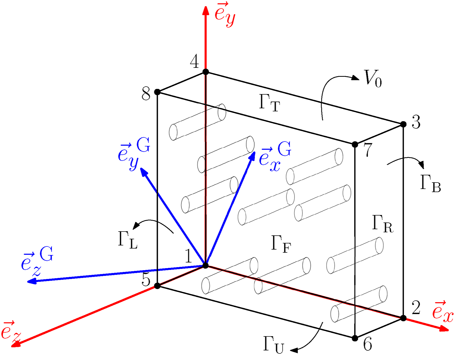

The standard periodic boundary conditions are applied to the RVE by prescribing linear tying relations that couple the displacements of nodes on opposite boundaries to the displacements of corner nodes 1, 2, 4, and 5. For this implementation, it is important that each node on one side of the RVE forms a unique pair with a node on the opposite side, while both nodes have equal in-plane positions. Subsequently, for each node pair on the right-left, top-bottom, and front-back boundaries, a linear tying relation is defined according to

${\overrightarrow{u}}_{\mathrm{R}}={\overrightarrow{u}}_{\mathrm{L}}+{\overrightarrow{u}}_{\left[2\right]}-{\overrightarrow{u}}_{\left[1\right]},$

(3a)

${\overrightarrow{u}}_{\mathrm{T}}={\overrightarrow{u}}_{\mathrm{U}}+{\overrightarrow{u}}_{\left[4\right]}-{\overrightarrow{u}}_{\left[1\right]},$

(3b)

${\overrightarrow{u}}_{\mathrm{F}}={\overrightarrow{u}}_{\mathrm{B}}+{\overrightarrow{u}}_{\left[5\right]}-{\overrightarrow{u}}_{\left[1\right]}.$

(3c)

In equations (3a)-(3c), ${\overrightarrow{u}}_{\chi }$ with χ = R, L, T, U, F, and B is the displacement of a node located on the boundary of the RVE and ${\overrightarrow{u}}_{\left[p\right]}$ is the displacement of a prescribed corner node p = 1, 2, 4, 5. Note that for nodes located on the edges and vertices, multiple possible tying relations can be defined.

Macroscopic uniaxial loading

Next, corner nodes 1, 2, 4, and 5 are prescribed such that a uniaxial macroscopic deformation along a chosen direction can be imposed. To this extent, the global Cartesian coordinate system $\left\{{\overrightarrow{e}}_x^{\mathrm{G}},{\overrightarrow{e}}_y^{\mathrm{G}},{\overrightarrow{e}}_z^{\mathrm{G}}\right\}$ is defined (see Figure 8). The direction ${\overrightarrow{e}}_x^{\mathrm{G}}$ is aligned with the uniaxial macroscopic loading direction. Furthermore, corner node 1 must be located at the origin and its displacements are prescribed for all three DOFs to prevent rigid body translations

${\overrightarrow{X}}_{\left[1\right]}={\overrightarrow{u}}_{\left[1\right]}=\overrightarrow{0}.$

(4)

In the computational homogenization framework introduced by Kouznetsova et al. in Ref. 37, a macroscopic deformation is applied to the microscopic RVE by relating the macroscopic deformation gradient F^M to the prescribed displacements of the corner nodes p = 1, 2, 4, 5 at the microscale, ${\overrightarrow{u}}_{\left[p\right]}$ , through equation (5)

${\overrightarrow{u}}_{\left[p\right]}=\left({\mathbf{F}}^{\mathrm{M}}-\mathbf{I}\right)·{\overrightarrow{X}}_{\left[p\right]}.$

(5)

Here, I is the second-order unit tensor and ${\overrightarrow{\mathrm{X}}}_{\left[\mathrm{p}\right]}$ is the position vector of corner node p in the undeformed configuration.

Uniaxial loading conditions are achieved if there is a prescribed deformation in the direction ${\overrightarrow{e}}_x^{\mathrm{G}}$ and traction-free conditions in the directions perpendicular to ${\overrightarrow{e}}_x^{\mathrm{G}}$ . This means that the following relations should hold for the macroscopic deformation gradient

${\overrightarrow{e}}_x^{\mathrm{G}}·{\mathbf{F}}^{\mathrm{M}}·{\overrightarrow{e}}_x^{\mathrm{G}}=F_{xx}^{\mathrm{M}}$

(6)

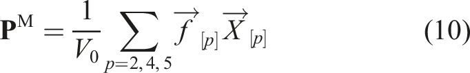
and the macroscopic stress σ ^M

$\begin{array}{l}{\overrightarrow{e}}_y^{\mathrm{G}}·{\mathbf{\sigma }}^{\mathrm{M}}·{\overrightarrow{e}}_y^{\mathrm{G}}={\overrightarrow{e}}_z^{\mathrm{G}}·{\mathbf{\sigma }}^{\mathrm{M}}·{\overrightarrow{e}}_z^{\mathrm{G}}={\overrightarrow{e}}_x^{\mathrm{G}}·{\mathbf{\sigma }}^{\mathrm{M}}·{\overrightarrow{e}}_y^{\mathrm{G}}=\\ {\overrightarrow{e}}_x^{\mathrm{G}}·{\mathbf{\sigma }}^{\mathrm{M}}·{\overrightarrow{e}}_z^{\mathrm{G}}={\overrightarrow{e}}_y^{\mathrm{G}}·{\mathbf{\sigma }}^{\mathrm{M}}·{\overrightarrow{e}}_z^{\mathrm{G}}=0.\end{array}$

(7)

Equation (6) is satisfied if corner nodes p = 2, 4, 5 are prescribed in the direction of the uniaxial load according to

$u_{\left[p\right]x}^{\mathrm{G}}={\epsilon }^{\mathrm{M}}{\overrightarrow{e}}_x^{\mathrm{G}}·{\overrightarrow{X}}_{\left[p\right]}=\left({\stackrel{.}{\epsilon }}^{\mathrm{M}}t\right){\overrightarrow{e}}_x^{\mathrm{G}}·{\overrightarrow{X}}_{\left[p\right]}$

(8)

where ${\epsilon }^{\mathrm{M}}=\left(F_{xx}^{\mathrm{M}}-1\right)$ is the macroscopic linear strain in the direction of the applied load. Similar to the experiments, the macroscopic deformation in the FE-simulations is strain rate controlled. For a constant strain rate ${\stackrel{.}{\epsilon }}^{\mathrm{M}}$ , the macroscopic strain at time t is written as ${\epsilon }^{\mathrm{M}}\left(t\right)={\stackrel{.}{\epsilon }}^{\mathrm{M}}t$ . Equation (8) is applied to the DOFs of the corner nodes in the local coordinate system by expressing ${\overrightarrow{e}}_x^{\mathrm{G}}$ in terms of the local coordinate system.

To satisfy equation (7), additional tying relations are defined for the displacements of corner nodes p = 2, 4, 5 orthogonal to the uniaxial load, $u_{\left[p\right]y}^{\mathrm{G}}$ and $u_{\left[p\right]z}^{\mathrm{G}}$ , where these displacements are also expressed in terms of the local coordinate system.

In the case of a 3D model, an additional boundary condition is required to prevent rigid body rotations around the uniaxial loading direction ${\overrightarrow{e}}_x^{\mathrm{G}}$ . ³⁴ This can be achieved by the requirement that the sum of all rotations is equal to zero, which is written as

${\displaystyle \sum }_{p=2,4,5}{\overrightarrow{e}}_x^{\mathrm{G}}·\left[{\overrightarrow{X}}_{\left[p\right]}\times {\overrightarrow{u}}_{\left[p\right]}\right]=0$

(9)

Macroscopic stress

The macroscopic first Piola–Kirchoff stress tensor P^M is used to compare the results from the FE-simulations to experiments. Following the computational homogenization framework by Kouznetsova et al. ³⁷ and equation (4), the macroscopic stress is calculated according to

${\mathbf{P}}^{\mathrm{M}}=\frac{1}{V_0}{\displaystyle \sum }_{p=2,4,5}{\overrightarrow{f}}_{\left[p\right]}{\overrightarrow{X}}_{\left[p\right]}$

(10)

where V₀ is the volume of the RVE in the initial undeformed configuration, and ${\overrightarrow{f}}_{\left[p\right]}$ is the external force acting on corner node p = 2, 4, 5.

Constitutive models

Elasto-viscoplastic matrix

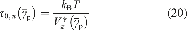
The 3D elasto-viscoplastic constitutive model, described by the authors in Ref. 25, is used to describe the rate-dependent behavior of neat PVDF at different temperatures. The model is an extension to the Eindhoven Glassy Polymer (EGP) constitutive model described by Van Breemen et al. ³⁸ The extension proposed in Ref. 25 entails a deformation-dependence of the activation volume and the rate-factor to accurately describe the rate-dependent large strain response of PVDF at different temperatures. Here, only the most important equations from the model are described. For a detailed description of the model, the reader is referred to Ref. 25.

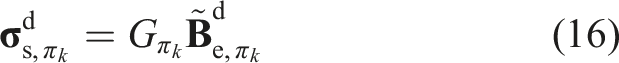
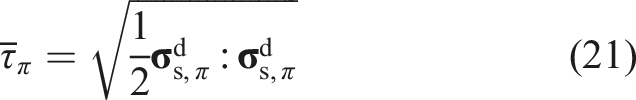
The total Cauchy stress σ is expressed as the sum of the hydrostatic stress σ ^h and the deviatoric stress σ ^d, denoted as

$\mathbf{\sigma }={\mathbf{\sigma }}^{\mathrm{h}}+{\mathbf{\sigma }}^{\mathrm{d}}$

(11)

The hydrostatic stress depends on the constant bulk modulus κ, and the volume change ratio J and is expressed as

${\mathbf{\sigma }}^{\mathrm{h}}=\kappa \left(J-1\right)\mathbf{I}$

(12)

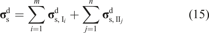
The deviatoric stress is split into the hardening stress ${\mathbf{\sigma }}_{\mathrm{r}}^{\mathrm{d}}$ and the driving stress ${\mathbf{\sigma }}_{\mathrm{s}}^{\mathrm{d}}$ as

${\mathbf{\sigma }}^{\mathrm{d}}={\mathbf{\sigma }}_{\mathrm{r}}^{\mathrm{d}}+{\mathbf{\sigma }}_{\mathrm{s}}^{\mathrm{d}}$

(13)

The mechanical analogue of the most general form of the EGP-model is shown in Figure 9.

Figure 9.

Mechanical analogue of the multi-process multi-mode EGP-model. ³⁸

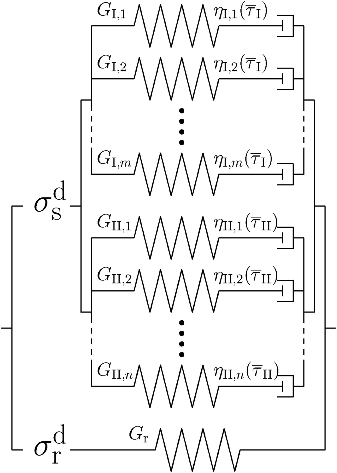
The hardening stress, denoted by the single spring at the bottom branch of the figure, represents the elastic response of the entanglement network. The hardening stress is modeled using the nonlinear Edward–Vilgis strain hardening model defined as

${\mathbf{\sigma }}_{\mathrm{r}}^{\mathrm{d}}=\frac{G_{\mathrm{r}}}{J}{\left(\stackrel{\sim }{\mathbf{B}}·\mathbf{Z}\right)}^{\mathrm{d}}$

(14)

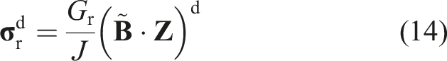
Here G_r is the hardening modulus, and $\stackrel{\sim }{\mathbf{B}}$ is the isochoric left Cauchy-Green strain tensor. The second-order tensor Z is a function of $\stackrel{\sim }{\mathbf{B}}$ and two parameters α_r and ξ_r, which represent the extensibility and mobility of the entanglement network, respectively.

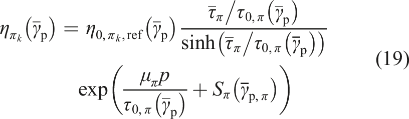
The top branch of the mechanical analogue in Figure 9 represents the driving stress. The deviatoric driving stress is represented by the nonlinear viscoelastic Maxwell elements, also called Maxwell modes. Each Maxwell element i is defined by a shear modulus G _i and a nonlinear Eyring viscosity η _i . The deformation of polymer materials can be attributed to one or more molecular processes being active simultaneously. In this model, it is assumed that these processes work in parallel. Furthermore, each molecular process can be represented by multiple Maxwell elements connected in parallel as well, according to Figure 9, to facilitate an accurate description of the nonlinear viscoelastic preyield behavior. For the multi-process multi-mode representation of the model in Figure 9, the deviatoric driving stress is defined as

${\mathbf{\sigma }}_{\mathrm{s}}^{\mathrm{d}}={\displaystyle \sum }_{i=1}^m{\mathbf{\sigma }}_{\mathrm{s},{\mathrm{I}}_i}^{\mathrm{d}}+{\displaystyle \sum }_{j=1}^n{\mathbf{\sigma }}_{\mathrm{s},{\text{II}}_j}^{\mathrm{d}}$

(15)

where m and n represent the total number of modes corresponding to process I and II, respectively. The deviatoric driving stress of mode k corresponding to process π is written as

${\mathbf{\sigma }}_{\mathrm{s},{\pi }_k}^{\mathrm{d}}=G_{{\pi }_k}{\stackrel{\sim }{\mathbf{B}}}_{\mathrm{e},{\pi }_k}^{\mathrm{d}}$

(16)

The subscript π corresponds to the respective molecular process and can be either I or II. The shear modulus of mode k corresponding to process π is represented by $G_{{\pi }_k}$ , and ${\stackrel{\sim }{\mathbf{B}}}_{\mathrm{e},{\pi }_k}^{\mathrm{d}}$ is the deviatoric part of the isochoric elastic left Cauchy–Green strain tensor.

The history- and time-dependence is accounted for by time-integration of the evolution equations for ${\stackrel{\sim }{\mathbf{B}}}_{\mathrm{e},{\pi }_k}$ and J. The evolution equation for ${\stackrel{\sim }{\mathbf{B}}}_{\mathrm{e},{\pi }_k}$ is defined as

${\stackrel{.}{\stackrel{\sim }{\mathbf{B}}}}_{\mathrm{e},{\pi }_k}=\left(\stackrel{\sim }{\mathbf{L}}-{\mathbf{D}}_{\mathrm{p},{\pi }_k}\right)·{\stackrel{\sim }{\mathbf{B}}}_{\mathrm{e},{\pi }_k}+{\stackrel{\sim }{\mathbf{B}}}_{\mathrm{e},{\pi }_k}·\left({\stackrel{\sim }{\mathbf{L}}}^{\mathrm{T}}-{\mathbf{D}}_{\mathrm{p},{\pi }_k}\right)$

(17)

Here, $\stackrel{\sim }{\mathbf{L}}$ denotes the isochoric velocity gradient tensor, and D is the rate of deformation tensor. A constitutive relation is required to solve for the evolution of ${\stackrel{\sim }{\mathbf{B}}}_{\mathrm{e},{\pi }_k}$ . Here, a non-Newtonian flow rule is used to relate the deviatoric driving stress to the plastic rate of deformation through the Eyring flow viscosity ${\eta }_{{\pi }_k}$ . This relation is defined as

${\mathbf{D}}_{\mathrm{p},{\pi }_k}=\frac{{\mathbf{\sigma }}_{\mathrm{s},{\pi }_k}^{\mathrm{d}}}{2{\eta }_{{\pi }_k}\left({\overline{\tau }}_{\pi },p,{\overline{\gamma }}_{\mathrm{p},\pi }\right)}$

(18)

where the Eyring flow viscosity is defined as

${\eta }_{{\pi }_k}\left({\overline{\gamma }}_{\mathrm{p}}\right)={\eta }_{0,{\pi }_k,\text{ref}}\left({\overline{\gamma }}_{\mathrm{p}}\right)\frac{{\overline{\tau }}_{\pi }/{\tau }_{0,\pi }\left({\overline{\gamma }}_{\mathrm{p}}\right)}{\sinh \left({\overline{\tau }}_{\pi }/{\tau }_{0,\pi }\left({\overline{\gamma }}_{\mathrm{p}}\right)\right)}\exp \left(\frac{{\mu }_{\pi }p}{{\tau }_{0,\pi }\left({\overline{\gamma }}_{\mathrm{p}}\right)}+S_{\pi }\left({\overline{\gamma }}_{\mathrm{p},\pi }\right)\right)$

(19)

here, ${\eta }_{0,{\pi }_k,\text{ref}}$ represents the reference viscosity of mode k corresponding to process π and τ_0,π is the characteristic stress, defined in equation (20), where k_B is the Boltzmann constant, T the absolute temperature, and $V_{\pi }^{*}\left({\overline{\gamma }}_{\mathrm{p}}\right)$ is the deformation-dependent activation volume of process π. The pressure-dependence is represented by the parameter μ _π . The equivalent shear stress ${\overline{\tau }}_{\pi }$ and the hydrostatic pressure p are defined according to equations (21) and (22), respectively

${\tau }_{0,\pi }\left({\overline{\gamma }}_{\mathrm{p}}\right)=\frac{k_{\mathrm{B}}T}{V_{\pi }^{*}\left({\overline{\gamma }}_{\mathrm{p}}\right)}$

(20)

${\overline{\tau }}_{\pi }=\sqrt{\frac{1}{2}{\mathbf{\sigma }}_{\mathrm{s},\pi }^{\mathrm{d}}:{\mathbf{\sigma }}_{\mathrm{s},\pi }^{\mathrm{d}}}$

(21)

$p=-\frac{1}{3}\text{tr}\left(\mathbf{\sigma }\right)$

(22)

The thermal history of the material is represented by S _π according to equation (23). The state parameter S_a,π describes the increase of the yield stress due to aging of the material, whereas the stress decrease due to strain softening is represented by the softening function $R_{\gamma ,\pi }\left({\overline{\gamma }}_{\mathrm{p},\pi }\right)$ in equation (24), where ${\overline{\gamma }}_{\mathrm{p},\pi }$ is the equivalent plastic strain

$S_{\pi }=S_{\mathrm{a},\pi }{R}_{\gamma ,\pi }\left({\overline{\gamma }}_{\mathrm{p},\pi }\right)$

(23)

$R_{\gamma ,\pi }\left({\overline{\gamma }}_{\mathrm{p},\pi }\right)={\left[\frac{1+{\left(r_{0,\pi }\hspace{0.17em}\exp \left({\overline{\gamma }}_{\mathrm{p},\pi }\right)\right)}^{r_{1,\pi }}}{1+r_{0,\pi }^{r_{1,\pi }}}\right]}^{\frac{r_{2,\pi }-1}{r_{1,\pi }}}$

(24)

The parameters r_0,π, r_1,π, and r_2,π are material-dependent parameters to be identified.

The equivalent plastic strain is computed from the equivalent plastic strain rate of the Maxwell mode with the longest relaxation time, which is assumed to be the first mode in the spectrum, that is, k = 1. The equivalent plastic strain rate is defined as

${\dot{\overline{\gamma }}}_{\mathrm{p},\pi }=\frac{{\overline{\tau }}_{{\pi }_1}}{{\eta }_{{\pi }_1}}$

(25)

here ${\overline{\tau }}_{{\pi }_1}$ and ${\eta }_{{\pi }_1}$ are the equivalent shear stress and the viscosity of the first mode of process π, respectively. ${\overline{\tau }}_{{\pi }_1}$ is calculated using the deviatoric driving stress of the corresponding mode ${\mathbf{\sigma }}_{\mathrm{s},{\pi }_1}^{\mathrm{d}}$ and equation (21).

In Ref. 25, the authors have shown that the rate-dependence of PVDF changes with increasing deformation. To incorporate this in the constitutive model, a deformation-dependent activation volume and reference viscosity is used. These material parameters are strain-dependent by means of the equivalent plastic strain, that is, $V^{*}\equiv V^{*}\left({\overline{\gamma }}_{\mathrm{p}}\right)$ and ${\eta }_0\equiv {\eta }_0\left({\overline{\gamma }}_{\mathrm{p}}\right)$ . Up to the yield point, V* and η₀ are assumed to be constant. Additionally, the equivalent plastic strain is assumed to be zero at the yield point. Two bilinear functions are used to describe the evolution of $V^{*}\left({\overline{\gamma }}_{\mathrm{p}}\right)$ and ${\eta }_0\left({\overline{\gamma }}_{\mathrm{p}}\right)$ , starting with a linear increase after which they remain constant at a certain level of equivalent plastic strain. The bilinear functions are defined as

$V^{*}\left({\overline{\gamma }}_{\mathrm{p}}\right)=\{\begin{array}{ll}{V}_{\mathrm{s}}^{*}+{\mathrm{\Phi }}_V{\overline{\gamma }}_{\mathrm{p}}& 0\le {\overline{\gamma }}_{\mathrm{p}}<{\overline{\gamma }}_{\mathrm{p},\mathrm{t}},\\ V^{*}\left({\overline{\gamma }}_{\mathrm{p}}={\overline{\gamma }}_{\mathrm{p},\mathrm{t}}\right)& {\overline{\gamma }}_{\mathrm{p}}\ge {\overline{\gamma }}_{\mathrm{p},\mathrm{t}},\end{array}$

(26)

${\eta }_0\left({\overline{\gamma }}_{\mathrm{p}}\right)=\{\begin{array}{ll}{10}^{\left[{\mathrm{\Phi }}_{{\eta }_0}{\overline{\gamma }}_{\mathrm{p}}+\log \left({\eta }_{0,\mathrm{s}}\right)\right]}& 0\le {\overline{\gamma }}_{\mathrm{p}}<{\overline{\gamma }}_{\mathrm{p},\mathrm{t}},\\ {\eta }_0\left({\overline{\gamma }}_{\mathrm{p}}={\overline{\gamma }}_{\mathrm{p},\mathrm{t}}\right)& {\overline{\gamma }}_{\mathrm{p}}\ge {\overline{\gamma }}_{\mathrm{p},\mathrm{t}}.\end{array}$

(27)

The parameters $V_{\mathrm{s}}^{*}$ and η_0,s are the initial values at the yield point, that is, ${\overline{\gamma }}_{\mathrm{p}}=0$ . Φ _V and ${\mathrm{\Phi }}_{{\eta }_0}$ determine the evolution of V* and η₀, and ${\overline{\gamma }}_{\mathrm{p},\mathrm{t}}$ denotes the equivalent plastic shear strain above which the parameters remain constant.

As a consequence, the spectrum of reference viscosities ${\eta }_{0,{\pi }_k,\text{ref}}$ is dependent on the equivalent plastic strain as well. Furthermore, the sum of all modal viscosities must equal the total reference viscosity at the yield point ${\eta }_0\left({\overline{\gamma }}_{\mathrm{p}}=0\right)$ . Therefore, each modal reference viscosity ${\eta }_{0,{\mathrm{I}}_k,\text{ref},\text{init}}$ is scaled with respect to the total reference viscosity ${\eta }_0\left({\overline{\gamma }}_{\mathrm{p}}=0\right)={\eta }_{0,\mathrm{s}}$ . The scaled modal reference viscosities, used in equation (19), are thus defined as

${\eta }_{0,{\mathrm{I}}_k,\text{ref}}\left({\overline{\gamma }}_{\mathrm{p}}\right)={\eta }_{0,{\mathrm{I}}_k,\text{ref},\text{init}}\frac{{\eta }_0\left({\overline{\gamma }}_{\mathrm{p}}\right)}{{\eta }_{0,\mathrm{s}}}$

(28)

Note that due to the deformation-dependence of the activation volume and the reference viscosities, the Eyring flow viscosity defined in equation (19) and the characteristic stress defined in equation (20) are now also dependent on the equivalent plastic strain, although these equations remain unchanged.

The parameters to describe PVDF at temperatures 23, 55, and 75°C were identified in Ref. 25 using a set of uniaxial compression and tension tests on pure PVDF. In that study it was reported that there is a substantial variety in the intrinsic behavior and yield kinetics of neat PVDF between the three testing temperatures. The microstructural evolution of PVDF under the influence of temperature was given as a probable cause for this variation, a phenomenon that was also reported in literature. Consequently, it does not seem realistic to characterize a single set of material parameters for the entire range of temperatures. Therefore, a distinct set of parameters is used for each temperature, spanning 3 microstructural regimes. The three sets of parameters that were identified in Ref. 25 are presented in Tables 2–5 in Appendix A. It is important to note that no additional parameter characterization is performed for the application of the constitutive model in the micromechanical model described in the present work. Hence, the properties of the neat PVDF are used without modifications.

Transversely isotropic fibers

Because the elastic strains in the fibers are assumed to remain small, a linear elastic transversely isotropic model is used to describe their behavior. The longitudinal direction of the fibers is aligned with the local ${\overrightarrow{e}}_z$ -direction and the plane of isotropy is the ${\overrightarrow{e}}_x$ - ${\overrightarrow{e}}_y$ plane according to Figure 8. The material is defined by the elastic constants shown in Table 1. ³⁹

Table 1.

Material parameters for the linear elastic transversely isotropic fibers.

Parameter	Value	Unit
E xx = E yy	15	[GPa]
E zz	225	[GPa]
G xy	15	[GPa]
G xz = G yz	7	[GPa]
ν xy	0.2	[-]
ν xz = ν yz	0.02	[-]

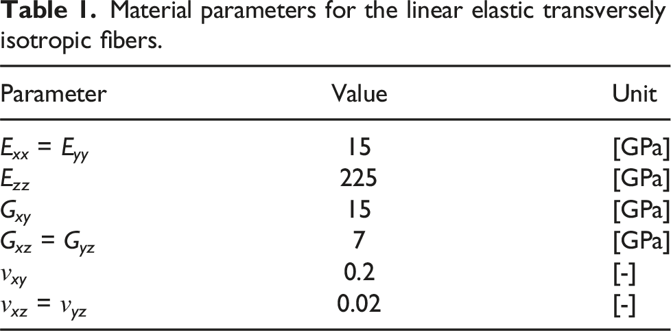
Perfect bonding between the fibers and matrix is assumed, because failure is not considered in this study.

Finite element model

The micromechanical finite element model is implemented in the FE package Abaqus CAE 2019. The fiber material is modeled using the standard anisotropic material model in Abaqus with the engineering constants defined in Table 1. The elasto-viscoplastic constitutive model described above is implemented as a UMAT user subroutine, based on Ref. 40.

The generation of the 3D geometry and discretization in Abaqus is split into 2 steps. First, the 2D geometry is defined using the in-plane dimensions of the RVE and the corresponding fiber coordinates as shown in Figure 7(b). This geometry is discretized using 8-node quadratic rectangular plane strain elements with reduced integration. Subsequently, the 2D-mesh is extruded in the out-of-plane direction, that is, along the longitudinal fiber orientation, over a length of 0.5 μm, resulting in an RVE discretized by 20-node quadratic hexagonal elements with reduced integration, that is, 8 integration points per element. All tying relations used for the periodic boundary conditions described in the Section Uniaxial periodic boundary conditions are implemented as linear constraints between corresponding DOFs. A mesh convergence study on the in-plane discretization resulted in an element size for the matrix between 0.15 and 0.4 μm, whereas a single element in the thickness direction was sufficient. The final 3D geometry and the corresponding finite element mesh are shown in Figure 10, which consists of 40279 elements and 283811 nodes.

Figure 10.

(a) The 3D finite element model used in the simulations and (b) the FE discretization of the in-plane geometry.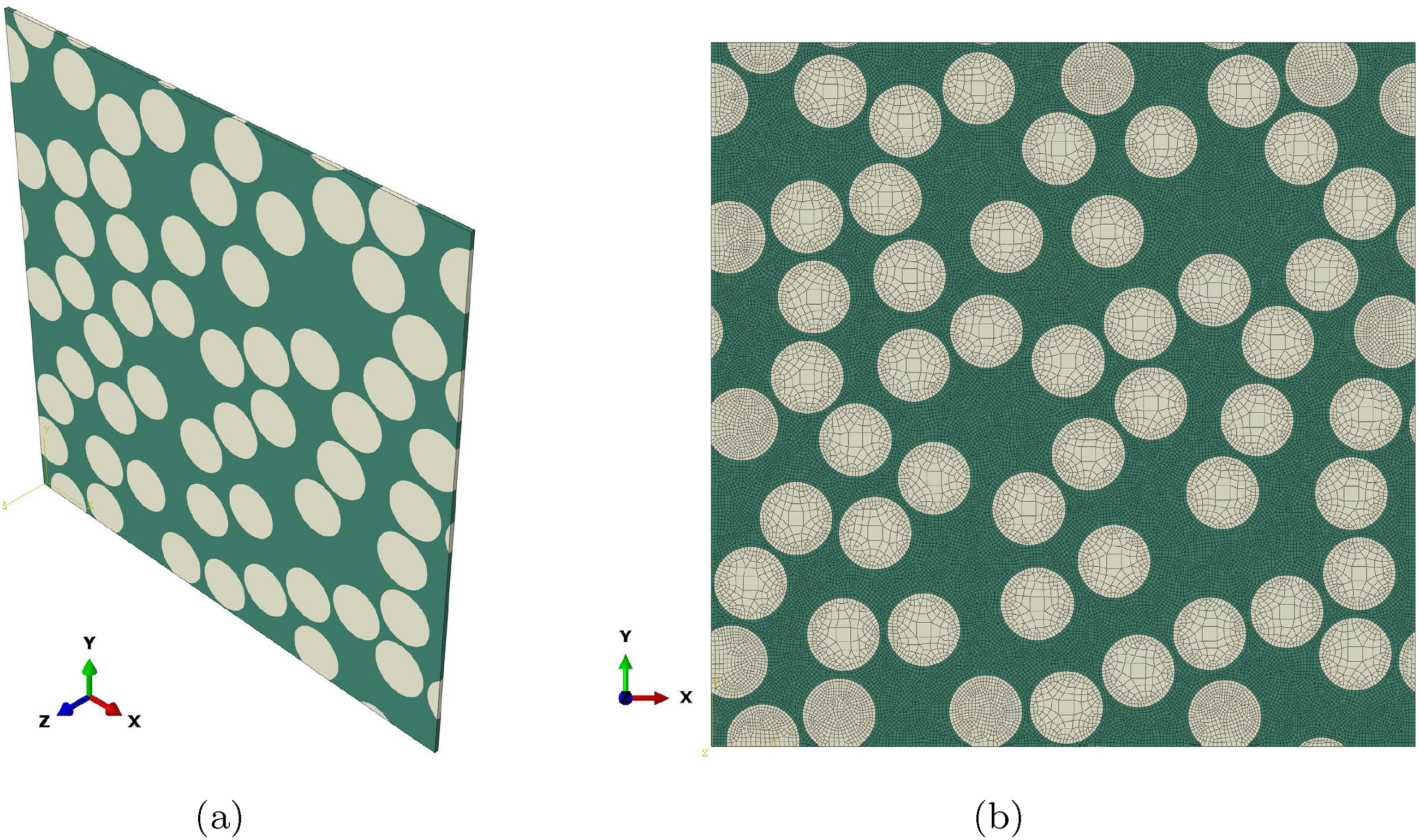

Results and discussion

First the average response obtained from the FE-simulations are compared to the experimental results. Subsequently, the local deformations at the microscale are analyzed in more detail.

Like the experiments, the macroscopic response of the FE-simulations is expressed in terms of the engineering stress and strain. To this extent, the magnitude of the normal component of the macroscopic first Piola–Kirchoff stress $P_{\mathrm{n}}^{\mathrm{M}}$ in the direction of the macroscopic load ${\overrightarrow{e}}_x^{\mathrm{G}}$ is computed as

$P_{\mathrm{n}}^{\mathrm{M}}={\overrightarrow{e}}_x^{\mathrm{G}}·{\mathbf{P}}^{\mathrm{M}}·{\overrightarrow{e}}_x^{\mathrm{G}}$

(29)

The macroscopic engineering strain is prescribed to the RVE according to equation (8). The same testing conditions that were used for the experiments are applied in the simulations. In all cases, the experimental data is represented by markers and simulation results are shown by solid lines.

Uniaxial tension

The predicted stress–strain results for transverse uniaxial tension at 23 and 75°C at three strain rates in the range 10⁻³ to 10⁻⁵ s⁻¹ are shown in Figure 11(a). The predictions show that the model accurately describes the rate-dependent mechanical behavior up to the experimental failure strain, although the rate-dependence of the material is relatively small. Similar to the experiments, the stress increases with increasing strain rate, whereas a higher temperature results in a stress decrease. The predictions of the transverse tensile response at a strain rate of 10⁻³ s⁻¹ at the three different temperatures 23, 55, and 75°C are shown in Figure 11(b), where a higher temperature results in lower stresses. Again, the micromechanical model adequately reflects the macroscopic response up to the experimental failure point. Near the experimental failure strain, the predictions at some conditions start to deviate from the experiments. This may be related to fiber-matrix debonding and damage initiation of the matrix, which are not incorporated in the model. This is also the reason that the point of failure is not predicted. Nevertheless, both comparisons demonstrate the added value of incorporating the elasto-viscoplastic material model, without the need for additional parameter characterization. Furthermore, the definition of the RVE geometry is of great importance for the accuracy of the model, as it was verified that an RVE having a lower or higher fiber volume fraction than the average fiber volume fraction, results in an under- or over-prediction of the experimental stress–strain response, respectively.

Figure 11.

Macroscopic response from the FE-simulations (solid lines) and experiments (markers) for uniaxial transverse tensile tests (θ = 90°) under different loading conditions. (a) Results at temperatures 23 and 75°C for different strain rates and (b) at strain rate 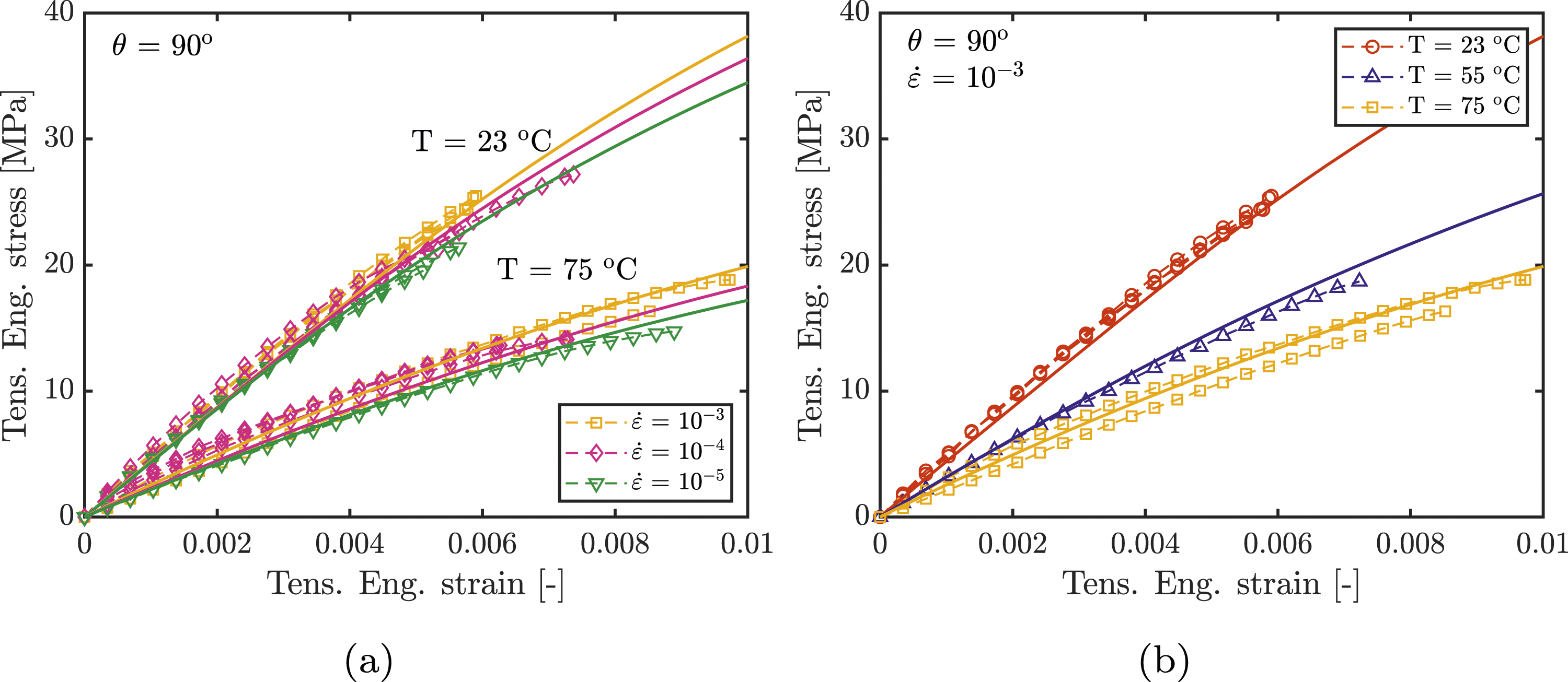$\stackrel{.}{\epsilon }={10}^{-3}{\mathrm{s}}^{-1}$ for varying temperatures.

Next, the stress fields in the micromechanical predictions are analyzed at the point that macroscopic failure is reached in the experiments. Macroscopic failure in the experiments is denoted as the final data point in the stress–strain curve. The local response is analyzed at this macroscopic strain. The local von Mises stress and hydrostatic stress for transverse tension at 23°C and strain rate $\stackrel{.}{\epsilon }={10}^{-3}{\mathrm{s}}^{-1}$ at ɛ^M = 0.59% is shown in Figure 12(a) and (b), respectively. The maximum von Mises stress can be found in matrix regions with high shear deformations, whereas the maximum hydrostatic stresses can be found in matrix regions loaded in the macroscopic tensile direction, denoted by the Y-direction in the figures. Similarly, the local response for transverse tension at 75°C and $\stackrel{.}{\epsilon }={10}^{-3}{\mathrm{s}}^{-1}$ at ɛ^M = 0.85% is shown in Figure 12(c) and (d), respectively. Compared to 23°C, the von Mises stresses are much lower, whereas the local maximum and minimum hydrostatic stresses are higher.

Figure 12.

Local von Mises stress and hydrostatic stress (both in MPa) for the transverse tensile test (a–b) at 23°C and strain rate 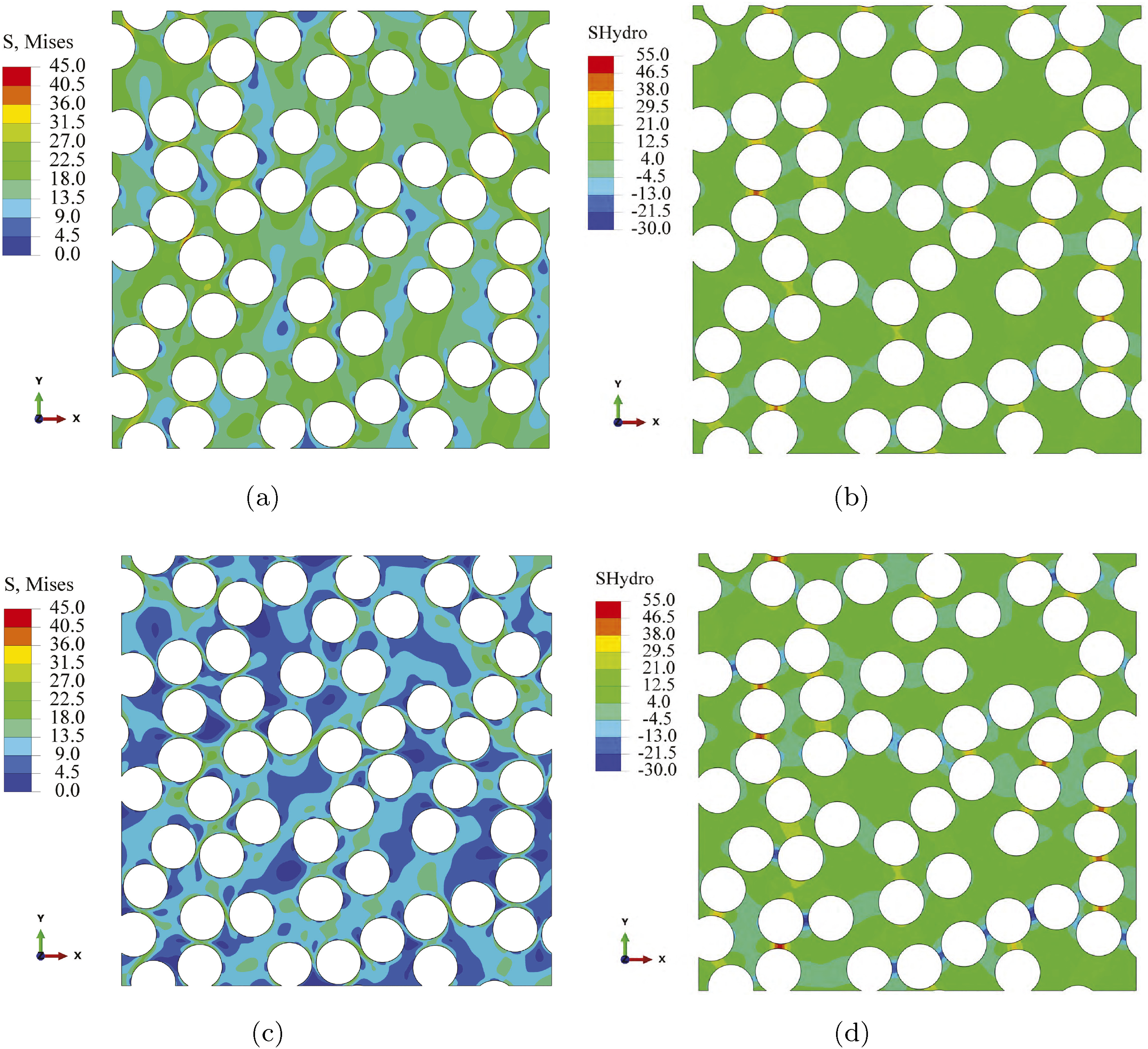$\stackrel{.}{\epsilon }={10}^{-3}{\mathrm{s}}^{-1}$ at ɛ^M = 0.59% and (c–d) at 75°C and strain rate $\stackrel{.}{\epsilon }={10}^{-3}{\mathrm{s}}^{-1}$ at ɛ^M = 0.85%. These are the macroscopic strains at which the composite material fails in the experiments.

To compare the local response at different testing conditions, the probability distribution of the hydrostatic stress and the von Mises stress in all integration points in the micromechanical model is analyzed at equal macroscopic strain.

The distribution of the von Mises stress and the hydrostatic stress for transverse tension at 23°C for strain rates between $\stackrel{.}{\epsilon }={10}^{-3}$ and $\stackrel{.}{\epsilon }={10}^{-5}{\mathrm{s}}^{-1}$ at a macroscopic strain equal to 0.56% are shown in Figure 13(a) and (b), respectively. ɛ^M = 0.56% is the experimental failure strain at $\stackrel{.}{\epsilon }={10}^{-5}$ . The macroscopic response for different strain rates, shown in Figure 11(a), is relatively similar. This is reflected in the local stress distributions as the hydrostatic stress distribution does not show significant differences for increasing strain rates, whereas the von Mises stress reveals a minor increase with applied strain rate.

Figure 13.

Probability distribution of the von Mises stress and hydrostatic stress (a–b) at macroscopic transverse strain ɛ^M = 0.56% for 23°C and strain rates 10⁻³ to 10⁻⁵ s⁻¹ and (c–d) at macroscopic transverse strain ɛ^M = 0.59% and strain rate 10⁻³ s⁻¹ at 23, 55, and 75°C.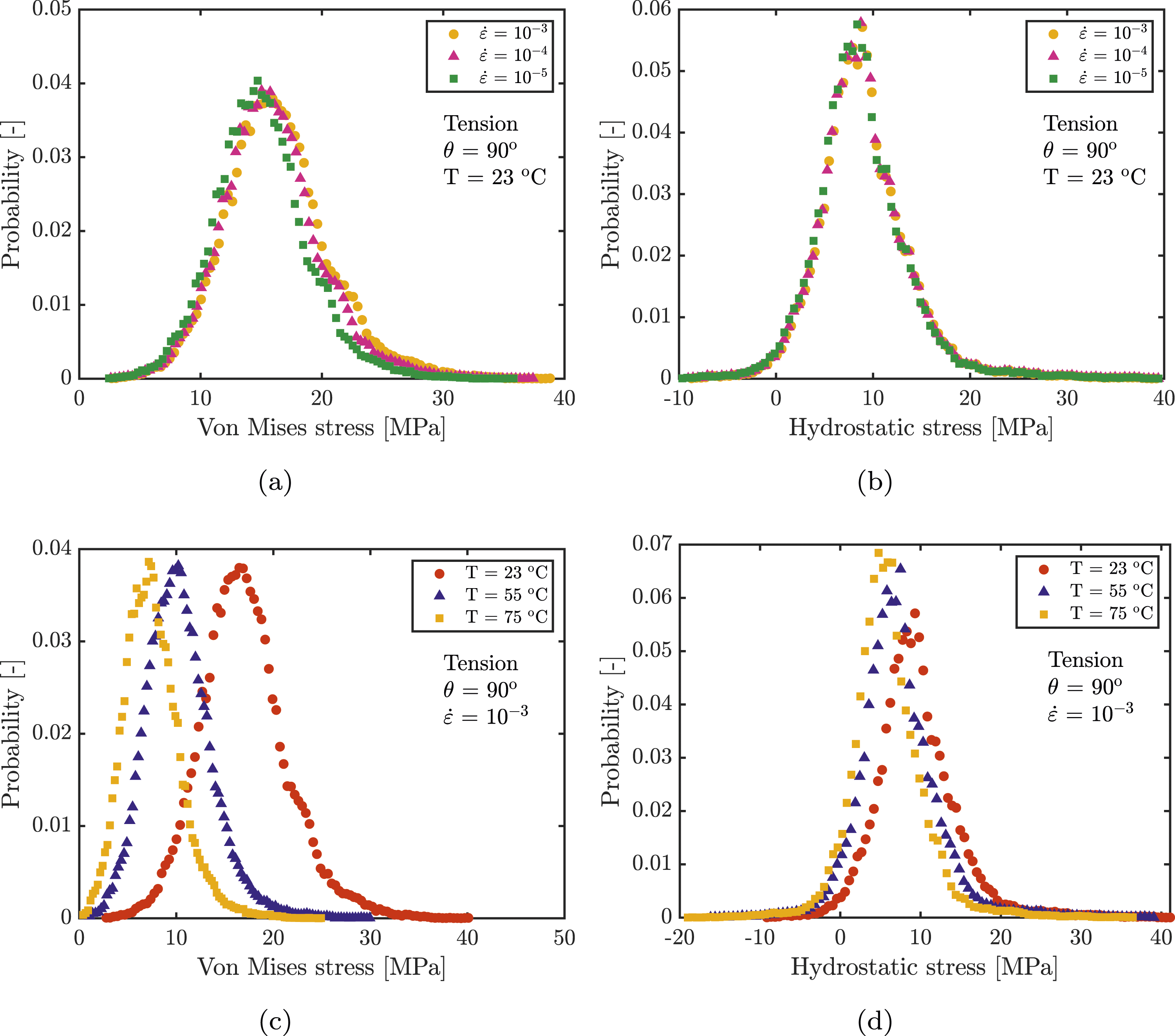

The distribution of the von Mises stress and the hydrostatic stress for transverse tension at $\stackrel{.}{\epsilon }={10}^{-3}$ for temperatures 23, 55, and 75°C at a macroscopic strain equal to 0.59% are shown in Figure 13(c) and (d), respectively. ɛ^M = 0.59% is the experimental failure strain at 23°C. The macroscopic response at different temperatures displays a wider variation, as demonstrated in Figure 11(b). Although the distribution of the local hydrostatic stress is comparable for all temperatures, the von Mises stress distribution shows a significant increase for decreasing temperature.

In Figure 14(a), the tensile response at a strain rate of 10⁻³ s⁻¹ at 55°C is shown for different fiber orientations. As expected, the stress response of the material increases for smaller angles θ as the fibers are loaded more in the fiber direction. The same results are shown in Figure 14(b) on a smaller scale, which reveals an adequate agreement between predictions and experiments for all angles. The probability distribution of the hydrostatic stress and the von Mises stress at 55°C and $\stackrel{.}{\epsilon }={10}^{-3}{\mathrm{s}}^{-1}$ at a macroscopic strain equal to 0.72% (the experimental failure strain for θ = 90°) for varying fiber orientations are given in Figure 14(c) and (d), respectively. In this case, the hydrostatic stress distribution shifts to lower stress levels for decreasing angle θ, while the distribution of the von Mises stress shifts to a higher level. Due to the off-axis loading, the shear deformations and shear stresses in the matrix are much higher compared to transverse loading of the composite, whereas the principal stresses decrease. This leads to the observed increase of the von Mises stress and decrease of the hydrostatic stress for smaller angles θ. The off-axis loading also results in higher shear loads and lower normal loads on the fiber/matrix interfaces compared to the dominance of normal loads for transverse tension. Furthermore, compared to the transverse tensile loading conditions where the equivalent plastic strain of the matrix is close to zero, an increase of the plastic deformation is observed for smaller angles θ. This larger plastic deformation and higher shear deformations are likely causing the experimental failure strain to increase.

Figure 14.

(a) Macroscopic response from the FE-simulations (solid lines) and experiments (markers) of uniaxial tension tests for varying fiber orientations at 55°C and 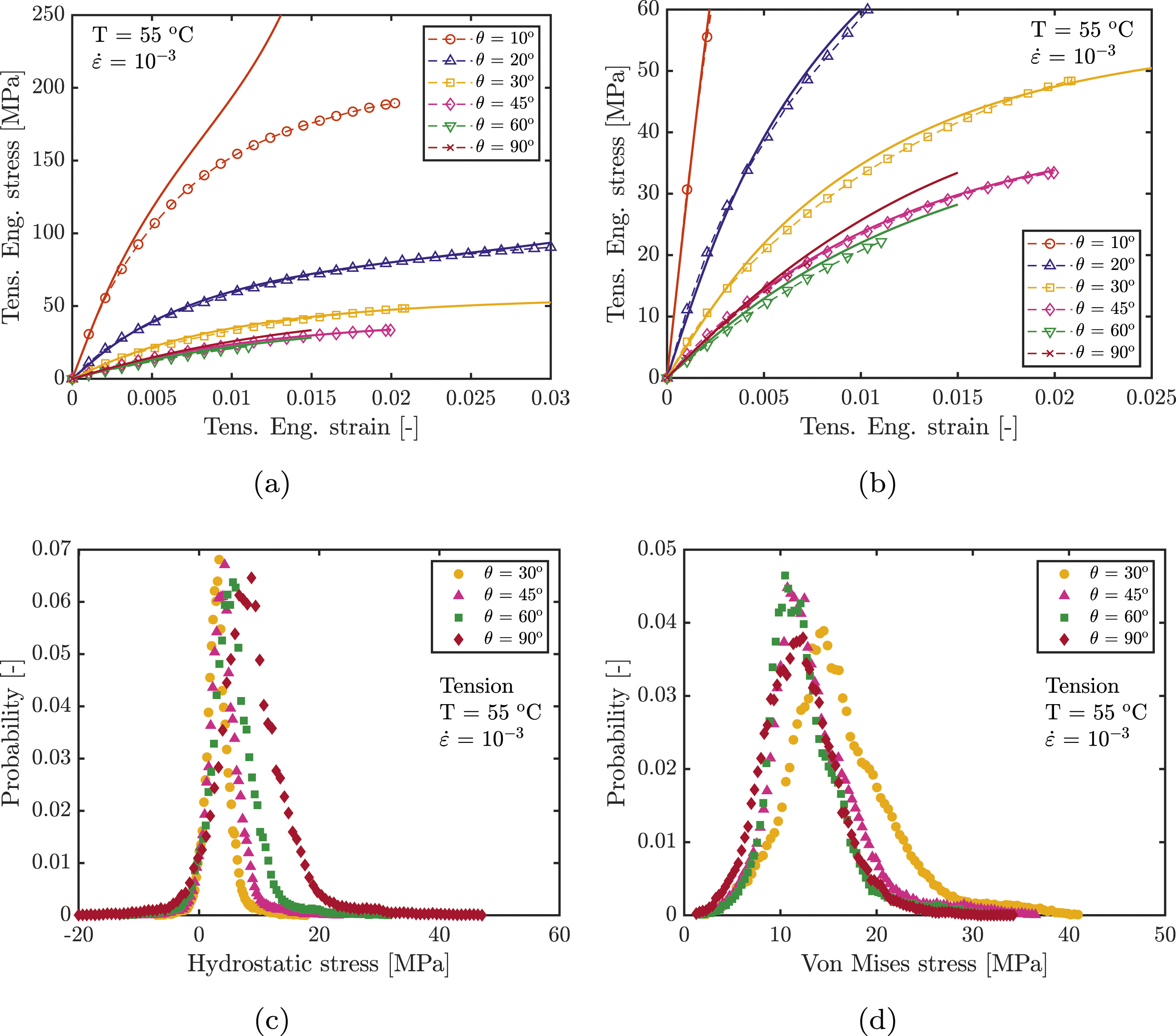$\stackrel{.}{\epsilon }={10}^{-3}{\mathrm{s}}^{-1}$ and (b) a zoom in on the bottom region of (a). Probability distribution of the (c) hydrostatic stress and (d) the von Mises stress at macroscopic strain ɛ^M = 0.72% for varying fiber orientations at 55°C and 10⁻³ s⁻¹.

Revisiting the prediction for the fiber orientation θ = 10° in Figure 14(a), only the response at small macroscopic strain is predicted adequately. After a strain of 0.5%, the micromechanical model overpredicts the response, even displaying hardening behavior. This can be explained by the rotation of the fibers when loaded under an angle. For a uniaxial macroscopic tensile load in y-direction, the macroscopic shear deformation $F_{yz}^{\mathrm{M}}$ should be zero, which is the case for the experiments due to the clamped ends of the specimens that are only allowed to move in the y-direction. Because the specimens used in the experiments are sufficiently long, not a single fiber is clamped at both ends, thereby preventing fiber rotation as much as possible. Although $F_{yz}^{\mathrm{M}}=0$ is also assumed for the uniaxial periodic boundary conditions described above, $F_{yz}^{\mathrm{M}}$ seems to be non-zero in the simulations. As a result, the preferential orientation of the fibers, when loaded in tension, rotates towards the direction of the applied load with increasing deformation. Consequently, part of the applied load to the composite is redistributed from shear load of the matrix towards tensile load of the fibers, giving rise to the hardening behavior observed in Figure 14(a). This effect is most pronounced for small angles θ. For example, the orientation of the fibers in the deformed configuration for a macroscopic load that is applied under an angle of θ = 45° and θ = 10° are compared at equal macroscopic strain ɛ^M = 2.0%. For a macroscopic load under θ = 45°, the orientation of the fibers in the deformed configuration rotated over an angle of only 1.2°, whereas for a macroscopic load under θ = 10° the orientation in the deformed configuration rotated by 7.5°. Hence, the relative deviation of the fiber orientation in the deformed configuration with respect to the macroscopic load direction is much larger for small angle θ than for a large angle θ. Hence, additional research is required to find a solution for the excessive rotation of the fibers and to obtain a more accurate prediction for the composite response at larger macroscopic deformations for small angle θ.

Uniaxial compression

The predictions of transverse uniaxial compression tests at 23 and 75°C at three strain rates in the range 10⁻¹ to 10⁻⁵ s⁻¹ are shown in Figure 15(a). The initial stiffness described by the simulations is in good agreement with the experiments for all cases. Furthermore, the stress response increases with increasing strain rate and decreasing temperature. At 75°C, the nonlinear response of the composite described by the simulations is also in adequate agreement with the experiments, although there is a minor overprediction at the highest strain rate. At 23°C, the rate-dependence predicted by the simulations remains only approximately in agreement with the experiments. Indeed, the compressive yield stress observed in the experiments is overpredicted by the simulations. There are two possible explanations for these overpredictions.

Figure 15.

Macroscopic response from the FE-simulations (solid lines) and experiments (markers) for uniaxial compression tests under different loading conditions. Transverse compression (a) at temperatures 23 and 75°C for different strain rates and (b) compression at 23°C and a strain rate of 10⁻³ for fiber orientations 0, 45, and 90°.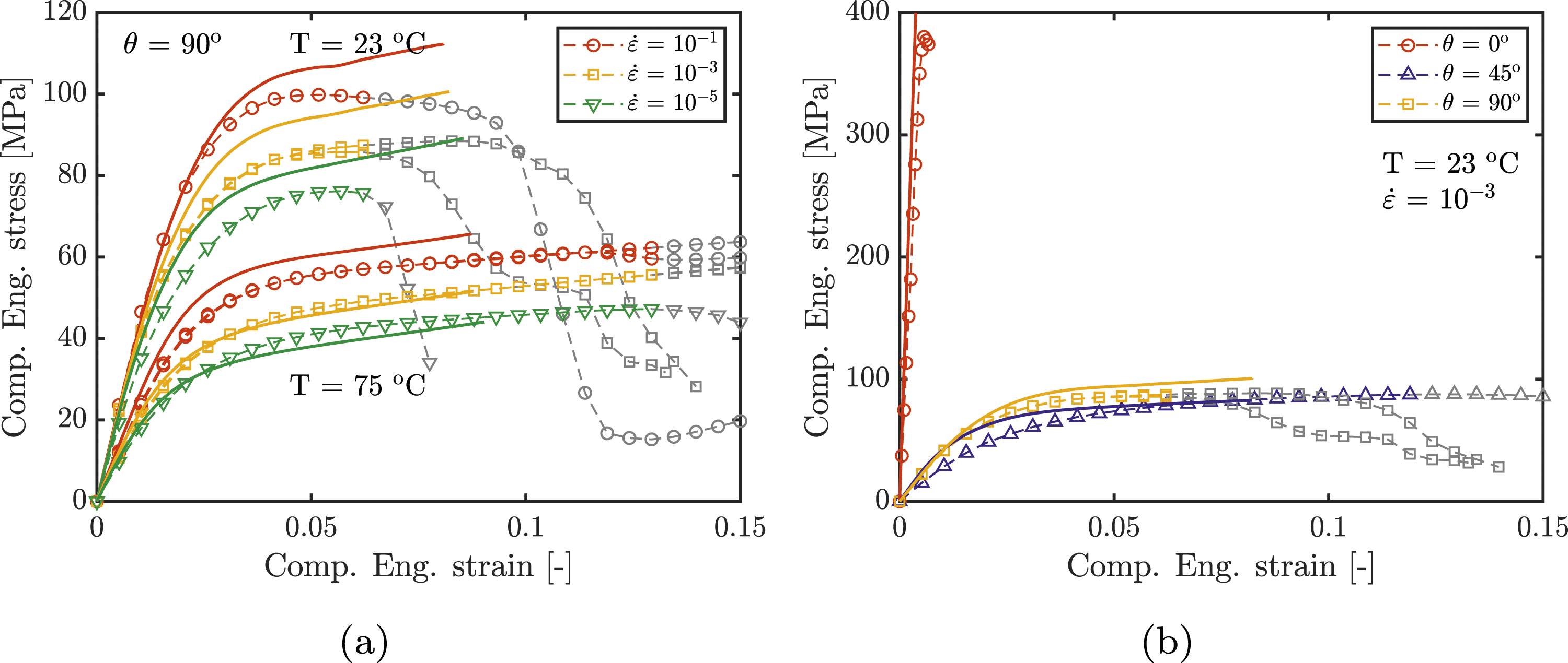

First, no fiber-matrix debonding is included in the FE-model and therefore the nonlinear response is fully attributed to plasticity in the PVDF matrix. The fact that the predictions at higher temperature and lower strain rate are in agreement with experiments, may also be due to the absence of fiber-matrix decohesion in the FE-model. At high temperatures and low strain rates, the stresses in the matrix are relatively low, which means that the loads on the interfaces between fibers and matrix are also lower. The deformation under these conditions is therefore dominated by matrix plasticity, which is accurately described by the micromechanical model. For lower temperatures and higher strain rates, the stresses in the matrix increase, resulting in higher loads on the fiber-matrix interfaces. These higher loads on the interfaces will trigger decohesion between fiber and matrix in the experiments.

The compressive response at 23°C at a strain rate of 10⁻³ s⁻¹ for fiber orientations of 0°, 45°, and 90° is shown in Figure 15(b). Obviously, if the fibers are loaded in their preferential direction (θ = 0°), the stiffness is the highest, which is captured by the FE-model. The experimental failure point is reached when a kinkband forms across the specimen. Due to the relatively small thickness of the FE-model, fiber bending and eventually kinkbands cannot be described.

The response of the sample with a fiber orientation of 45° is shown in blue. The yield stress predicted by the model is in agreement with the experiment. There is however a difference between the prediction and experiment in the small strain region. During the experiments, shear band formation at the surface of the specimen is observed at relatively small strains, whereas these shear bands do not occur in the simulations. Furthermore, due to the fiber orientation of 45°, the specimen also displaces in a horizontal direction in the experiments, resulting in a more compliant response. This off-axis movement is prevented by the periodic boundary conditions in the simulations.

Conclusion

In this study, the so far unexplained, rate- and temperature-dependent mechanical behaviour of UD carbon fiber-reinforced PVDF is investigated. Uniaxial tension and compression experiments were performed to investigate the macroscopic stress–strain behaviour of the UD composite at varying constant strain rates, temperatures, and fiber orientations. Analysis of microscopy images of a cross section of the composite was performed to retrieve the microstructural morphology. A micromechanical FE-model was developed to investigate the mechanical behavior of UD carbon fiber-reinforced PVDF. The microscopic analysis was used to determine the RVE geometry for the micromechanical model. To describe the nonlinear rate- and temperature-dependent behaviour of the PVDF matrix, an elasto-viscoplastic material model was used. An efficient algorithm was implemented for the simulation of macroscopic uniaxial loading in any direction in combination with periodic boundary conditions.

The macroscopic response obtained from the finite element simulations was compared to the experimental stress–strain response. An adequate agreement was found between the predictions from the FE-simulations and the experiments for most loading conditions. Both the rate and temperature dependence of the composite material is well described by the model, as well as the different responses for varying fiber orientations. Some limitations of the model have been identified when the fiber orientations are close to the macroscopic loading direction, due to excessive rotations of the fibers. Further improvements can also be made by introducing damage mechanisms to capture fiber-matrix debonding and damage of the PVDF matrix.

The three main advantages of the presented model are the straightforward generation of the 3D RVE, an accurate constitutive model to describe the nonlinear rate- and temperature-dependent matrix behavior and the application of off-axis loading conditions on a thin 3D RVE. The general structure of the presented framework allows for application of the model to different fiber-reinforced polymers to facilitate efficient analysis of these composite materials. Eventually, homogenization techniques may be employed to upscale the model and enable efficient analysis of large composite structures while still incorporating the relevant mechanisms at the microscale.

Supplemental Material

Supplemental Material - A periodic micromechanical model for the rate- and temperature-dependent behaviour of unidirectional carbon fiber-reinforced PVDF

Supplemental Material for A periodic micromechanical model for the rate- and temperature-dependent behaviour of unidirectional carbon fiber-reinforced PVDF by Tom Lenders, Joris JC Remmer, Tommaso Pini, Peter Veenstra, Leon E Govaert, and Marc GD Geers in Journal of Reinforced Plastics and Composites.

Supplemental Material

Supplemental Material - A periodic micromechanical model for the rate- and temperature-dependent behaviour of unidirectional carbon fiber-reinforced PVDF

Supplemental Material for A periodic micromechanical model for the rate- and temperature-dependent behaviour of unidirectional carbon fiber-reinforced PVDF by Tom Lenders, Joris JC Remmer, Tommaso Pini, Peter Veenstra, Leon E Govaert, and Marc GD Geers in Journal of Reinforced Plastics and Composites.