
Abstract
Textbooks commonly misrepresent the effects of market entry and exit by consumers and producers as parallel shifts of linear market demand and supply curves. Such portrayals are inconsistent with the underlying premise that a market-level curve is the horizontal summation of individual-level curves. A more accurate depiction is a pivot: entry flattens (and exit steepens) a market-level curve. Reconceiving the effects of entry and exit as pivoting, rather than shifting, the curve has important implications for own-price elasticities, consumer surplus, producer surplus, the incidence of taxation, and the competitive market adjustment to a long run equilibrium.
Keywords
Introduction
Microeconomics textbooks, at both the principles and intermediate levels, commonly portray individual supply and demand curves as linear and include some version of the following three statements regarding demand, with analogous statements regarding supply.
1
* The market demand curve is the horizontal summation of individual buyers’ demand curves. * When buyers enter (exit) the market, the market demand curve shifts outward (inward). * The own-price elasticity of market demand depends on the nature of the good, the availability of substitutes, consumers’ incomes, and the length of time buyers have for adjusting purchases.
This paper shows that if the first claim is true, then the second is false and the third is deficient.
The following section demonstrates that, because market-level curves are constructed as the horizontal sums of individual-level curves, it is impossible for entry or exit to shift a downward-sloping market demand or upward-sloping market supply curve in the mathematical sense. Rather, as shown next, entry and exit cause a market-level curve to pivot, either around its vertical axis or another pivot point, flattening with entry and steepening with exit. Consequently, a complete list of the factors influencing the own-price elasticity of market demand (supply) should include the number of consumers (producers) in the marketplace. The Implications section demonstrates why the difference between a shift and a pivot is important: in addition to the inconsistencies between lessons, the failure to properly account for the effect of entry and exit generates incorrect results regarding elasticity, consumer surplus, producer surplus, tax incidence, and competitive market adjustment to a long run equilibrium. The penultimate section briefly considers nonlinear functions, and the final section concludes.
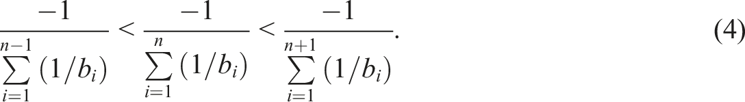
The Impossibility of Shifts
By definition, an inward or outward shift of a linear curve requires the intercept to change while the slope remains constant (Soper, 2004); thus, a shift connotes a parallel movement. Most textbooks correctly describe the market demand (supply) curve as the horizontal summation of individual demand (supply) curves, which are almost always assumed to be linear. That construction implies that neither entry nor exit can cause the curve to shift. To demonstrate this, we offer the following theorem. 2
If all consumers have negatively-sloped linear demand functions, then entry flattens and exit steepens the slope of the market demand curve.
Let each of n consumers have the demand function Thus, as consumers enter or exit, the market demand curve cannot shift in a parallel manner; it becomes flatter with entry and steeper with exit. An analogous argument applies to upward-sloping supply curves.


Entry and Exit Cause Pivots
We next examine the effects of entry and exit on the vertical intercept of a linear curve. First, note that a shift would imply that the vertical intercept of a demand (supply) curve necessarily rises (falls) with entry and falls (rises) with exit. That, however, need not be the case.
Consumer Entry
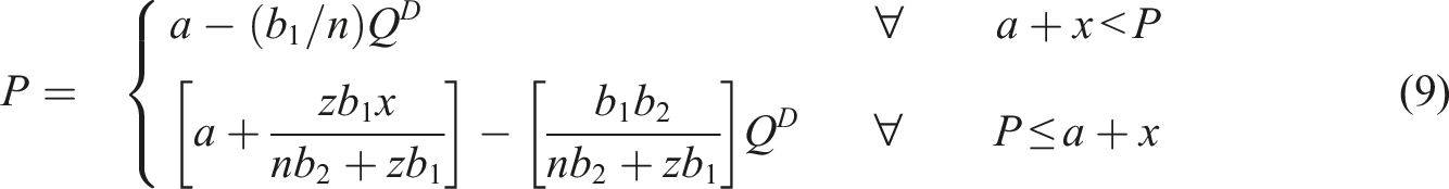
To isolate the effect of entry on demand, suppose that there are initially n consumers, each having the demand curve

Now let z new consumers enter the market, each of whom has the individual demand function

Consider three cases. First, suppose x > 0, so that the new entrants are willing to pay more than incumbent consumers for their first unit of the good. Then for

The new market demand curve is then a combination of two linear functions, equations (6) and (7):
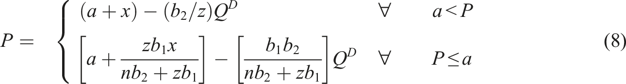
In this case, the market demand curve shifts upward and pivots, or kinks outward, at Market demand pivots outward in response to consumer entry. (A) x > 0 (B) x < 0 (C) x = 0.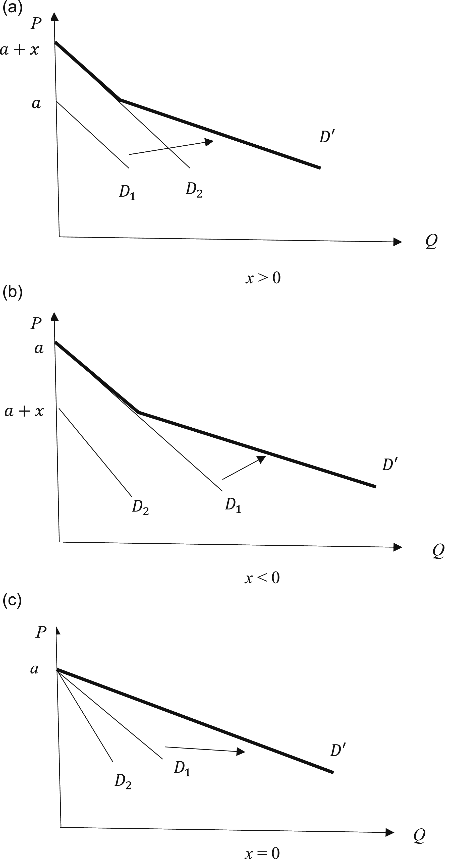
As a second case, suppose x < 0, so that the new consumers are not willing to pay as much as the incumbent consumers for their first unit of the good. Then at the highest prices (
This is shown in panel B of Figure 1, where the original market demand curve is again labeled
For the third case, suppose

This case is shown in Panel C of Figure 1. Note that in the limit, entry makes the slope approach zero and the market demand curve becomes nearly horizontal. Thus, the equilibrium price (
A Classroom Example
Market Demand as the Horizontal Sum of Individual Demands.
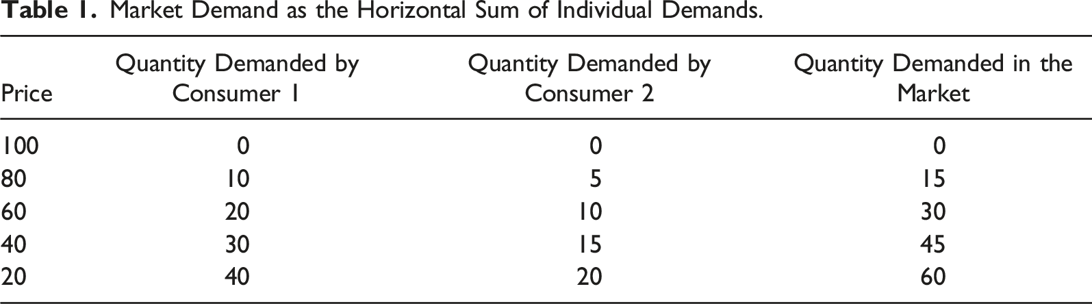
The general intuition can be explained as follows. If the price is so high that each consumer would buy, say, only one unit of the good, then when new consumers enter the market, the quantity demanded in the market increases only by the number of new consumers; but if the price is low, so that each consumer would buy multiple units, then when new consumers enter, the quantity demanded in the market increases by a multiple of the number of new consumers. For this reason, entry flattens the curve, and by the same logic, when consumers exit the market, the market demand curve becomes steeper, as discussed in more detail below. 4
Surprisingly, some textbooks correctly illustrate the market demand curve as being flatter than each individual demand curve, but fail to explicitly mention the difference in slope, and subsequently proceed to both describe in words and portray in diagrams the effect of entry (exit) by consumers as a parallel outward (inward) shift of the market demand curve.
Because we teach students that the market-level curve is the horizontal summation of individual curves, consistency requires that we depict market entry and exit as altering the slope and elasticity of the market-level curve, rather than shifting it in a parallel manner.
Consumer Exit
The analysis above indicates that if all consumers have linear demand curves, then the market demand curve will be nonlinear, unless all the individual demand curves have the same vertical intercept. Reversing the logic, if the market demand curve is linear, then either the individual demand curves are all linear and have the same vertical intercept, or at least one of the component curves has a higher vertical intercept and is kinked inward. These possibilities are depicted in Figure 2. In Panel A, curve Market demand pivots inward in response to consumer exit.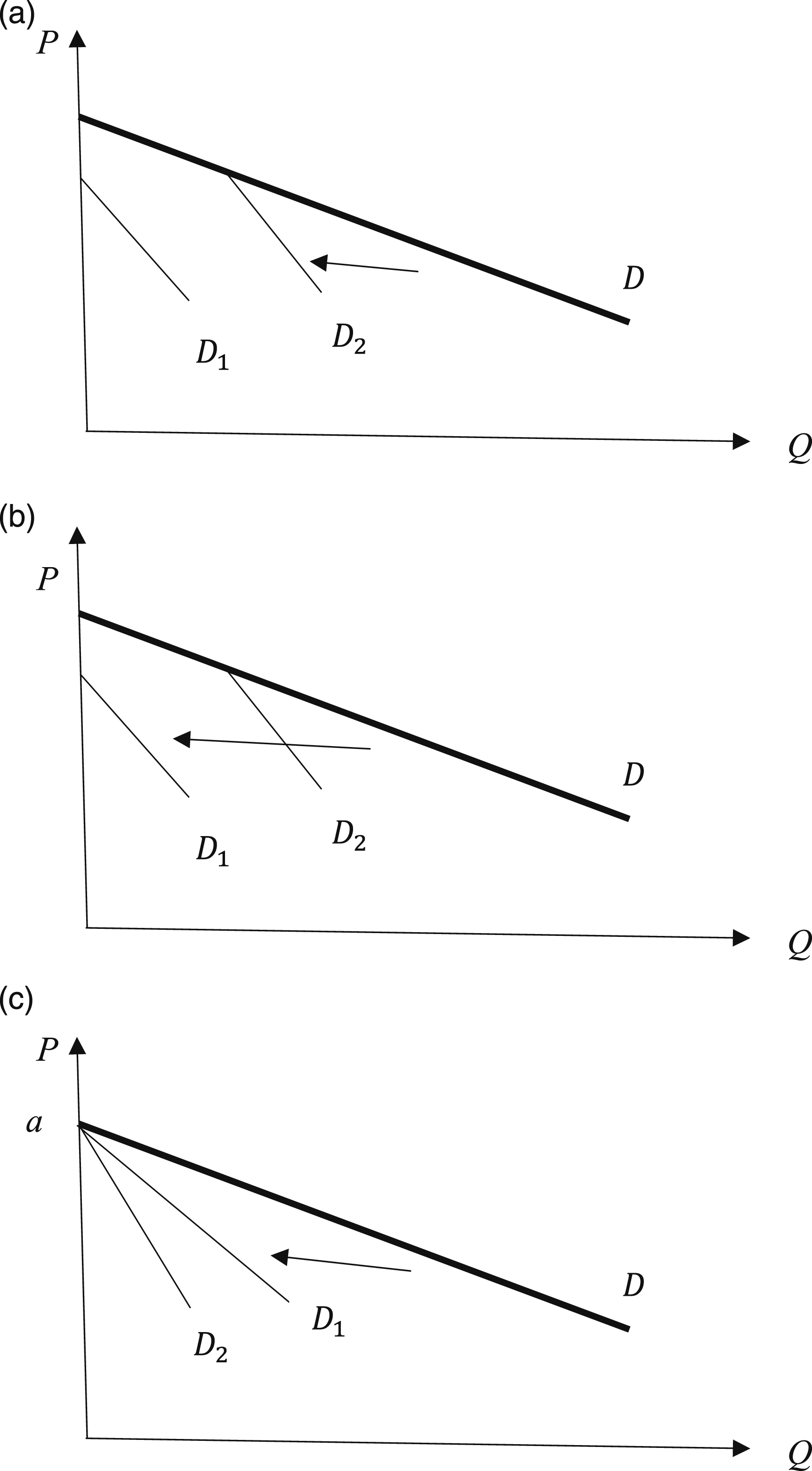
Market Supply
The analysis of supply is analogous to that of demand, so we will only briefly summarize it. An individual producer’s short run supply curve is the portion of its marginal cost curve that lies above average variable cost (AVC); the firm shuts down at prices below AVC, so the supply curve is discontinuous before it reaches the horizontal axis. Nonetheless, the individual producer’s supply function is often written as a simple linear equation with a positive slope and either a positive, zero, or negative vertical intercept.
Again, there are three cases. If new entrants are able to bring their initial units of the good to the market at lower cost than the incumbent producers, so that the vertical intercept of the entrants’ collective supply curve is lower than that of the incumbents’ supply curve, then at the lowest prices, only the supply of the new entrants is relevant, while at higher prices, the supply of all producers is relevant. This is depicted in Panel A of Figure 3, where Market supply pivots outward in response to producer entry.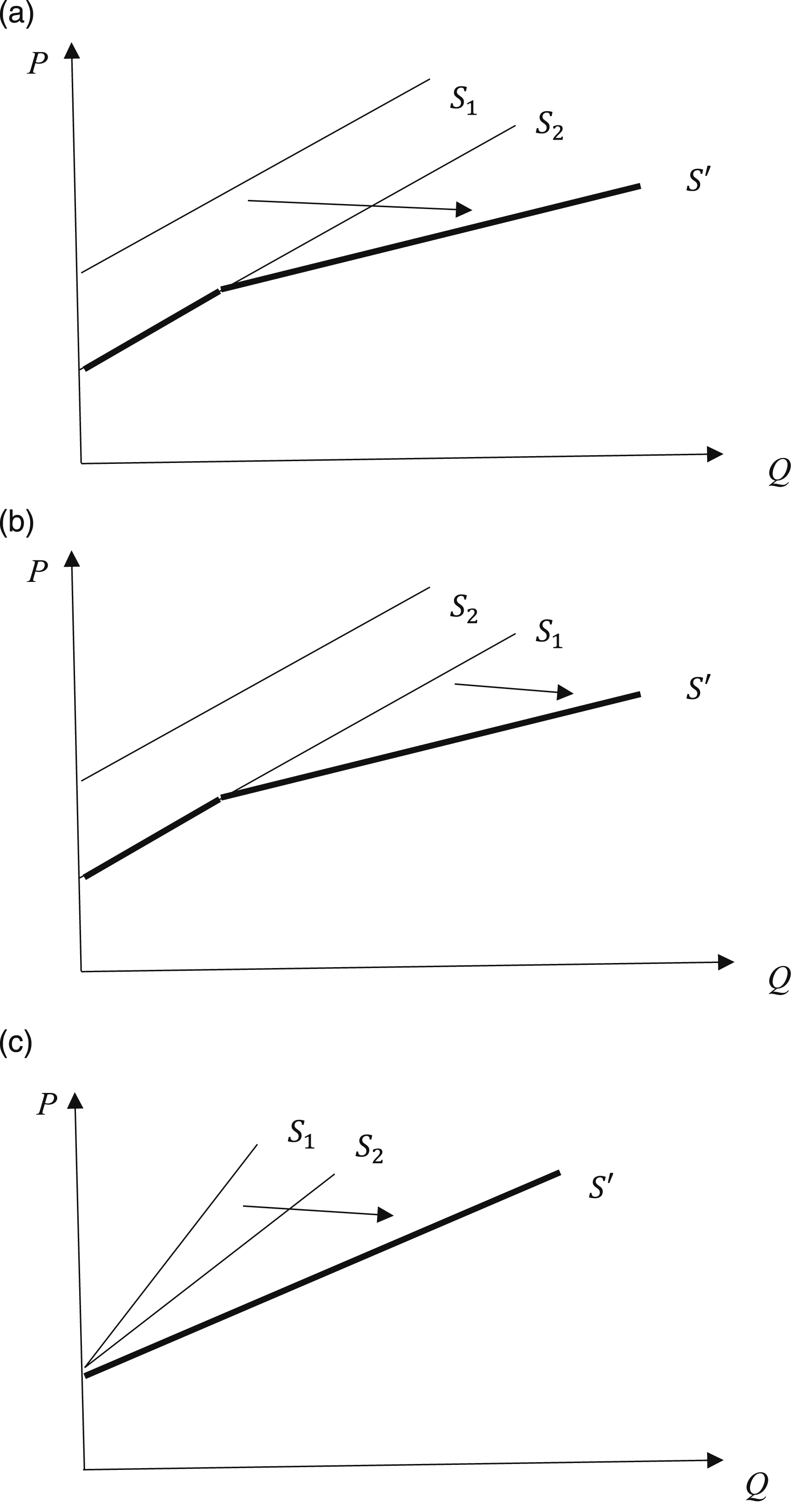
Conversely, if new producers are only able to bring their first units of output to the market at higher prices than incumbent producers, then at the lowest prices, only the original market supply curve,
The third possibility is that the new producers have the same costs as incumbents, so the supply curves of the two groups have the same vertical intercept; then entry causes the market supply curve to pivot clockwise around the vertical intercept, as in Panel C of Figure 3. 5
Finally, consider the exit of producers. If the original market supply curve is linear, then either all component supply curves have the same intercept, or one of the component curves has a lower vertical intercept and is nonlinear. In Panel A of Figure 4, curve Market supply pivots inward in response to producer exit.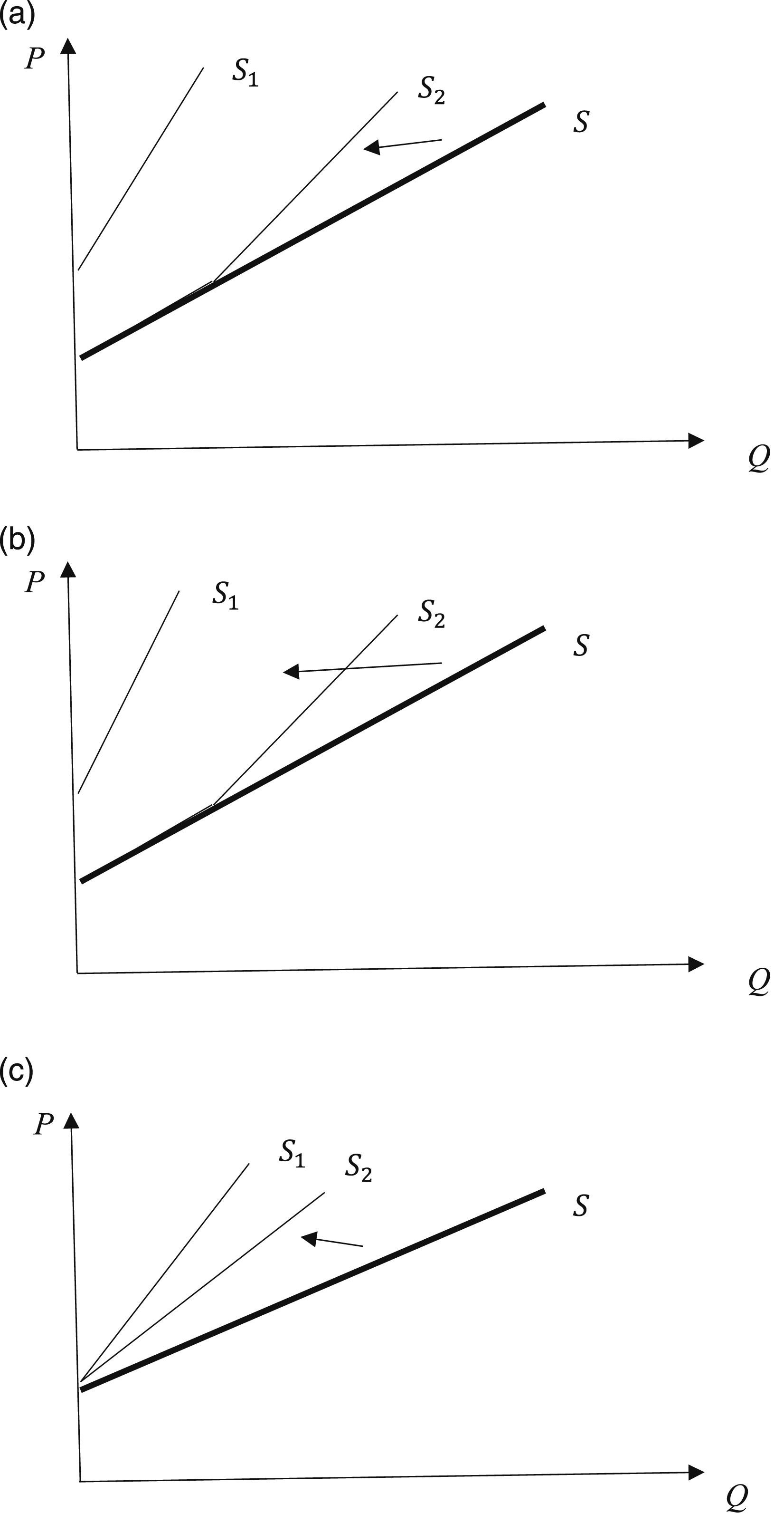
Though we have presented multiple scenarios for completeness, it may be simplest to present entry and exit in introductory courses as pivoting the market demand and supply curves around their vertical intercepts, as depicted in Panel C of each diagram above. Although this assumes a common intercept for demand curves and a common intercept for supply curves, it is more plausible than suggesting that entry or exit causes parallel shifts of the market-level curve. 7
Implications: Elasticity, Tax Incidence, Consumer Surplus, Producer Surplus, and Market Adjustment
In this section, we demonstrate that the traditional depiction of entry or exit as a shift gives false impressions of the changes in elasticity, tax incidence, consumer surplus, producer surplus, and the market adjustment mechanism.
Arc Elasticity of Demand
Although slope and elasticity are not the same, for linear functions there is a close relationship between the two, such that a more elastic curve has a flatter slope, and a less elastic curve is steeper. There are, of course, several different methods of calculating a price elasticity; to compare the overall elasticity of two different demand curves, we adopt Lerner’s (1933) arc elasticity metric as recommended by Seldon (1986), in which percentage changes are calculated relative to the lower values of price and quantity. To distinguish arc elasticities from point elasticities, we use
In the positive quadrant, where 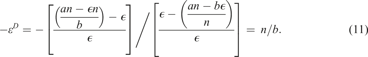
Equation (11) confirms that as consumers enter the market and
The list of factors affecting the price elasticity of demand that appears in textbooks typically includes the nature of the good (e.g., whether it is a necessity or a luxury), the availability of substitutes, consumers’ incomes (or equivalently, the share of consumers’ budgets taken by the good in question), and the length of time that consumers have for adjusting their purchases. These are correct insofar as they apply to individual demand curves, but the discussion of elasticity usually follows the presentation of market demand, leaving the impression that this is a comprehensive list of factors affecting elasticity at the market-level. Moreover, empirical examples of price elasticities of demand taken from various industries are often presented as part of the lesson, confirming the impression that the list applies to the elasticity of market demand. (Indeed, an individual consumer’s price elasticity should not matter in a competitive market). According to equation (11), the litany of factors influencing the own-price elasticity of market demand should also include entry and exit by consumers.
Arc Elasticity of Supply
To see the effect of entry and exit on the price elasticity of supply, suppose that there are m producers, each having the individual supply function
First, consider 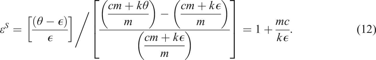
Notice that with
Another difference is also apparent. If
For 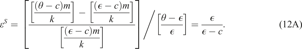
Here, a change in m alters the slope but not the overall arc elasticity of the supply curve. In contrast, changes in the intercept do affect the elasticity; in particular, if the market supply curve shifts outward (inward), it becomes more (less) inelastic. Indeed, if exit is portrayed as a parallel inward shift of the supply curve such that an originally negative c increases into positive values, then it is possible for an inelastic supply curve to become elastic if enough producers exit the market—a rather counterintuitive result.
Finally, if
Thus, as with demand, the manner in which the entry (or exit) of producers is portrayed has an important effect on how the elasticity of the resulting market supply curve is perceived. The factors listed by textbooks as affecting the price elasticity of supply ought to include entry and exit by producers, but typically do not. 9
Point Elasticities at Equilibrium
The two subsections above used arc elasticity measures to examine the overall price elasticities of demand and supply curves in isolation. Of course, as most textbooks explain, the elasticity changes at various points along a linear demand curve, being elastic at high prices and inelastic at low prices. Here, we consider the difference between a pivot and a shift of each curve as it affects price elasticity at the point of equilibrium
With the linear demand and supply equations above, the equilibrium quantity is

The absolute value of the price elasticity of demand at the point of equilibrium is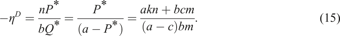
Equation (15) indicates that a demand curve that passes through any given equilibrium point exhibits greater elasticity when there is a greater value of n. Comparing a pivot of demand (an increase in n) to a shift of demand (an increase in a) that would result in the same new equilibrium, the pivot increases the point elasticity of demand more than the shift. 10
We perform a similar analysis of supply. At equilibrium, the point elasticity of supply with respect to price is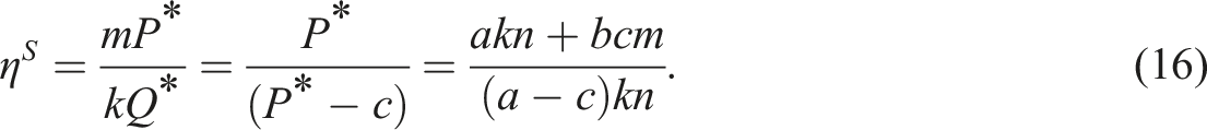
Like the arc elasticity of supply, the point elasticity depends on c; in particular,
Additionally, as noted above, when
Tax Incidence
Most textbooks rightly explain that the incidence of a tax falls primarily on the side of the market with the least elastic behavior. Because market entry or exit by consumers (producers) can change the own-price elasticity of demand (supply), it can also affect the incidence of taxes. In particular, the consumers’ share of the tax burden is related to the elasticities in the neighborhood of equilibrium according to


Holding b and k constant, equation (19) shows that changes in tax incidence depend entirely on changes in n and m. In particular, entry on one side of the market redistributes the tax incidence toward the other side. The opposite is also true: exit by buyers or sellers forces the remaining members of that group to bear a greater tax burden. Consider, for example, the Great Resignation—the large-scale withdrawal of workers from the labor force (Faccini, et al. 2022). This should cause the labor supply curve to pivot inward, becoming steeper and redistributing the incidence of payroll taxes away from employers and toward the remaining employees. By contrast, a parallel shift of the labor supply curve would leave the tax incidence unchanged.
New Consumers and Consumer Surplus
With linear supply and demand curves, the consumer surplus (CS) at equilibrium is the area of the triangle bounded by the vertical axis, the demand curve, and the equilibrium price. Thus,

Notice that, because
Consider three distinct cases. First, if supply is horizontal (i.e., perfectly elastic), so that 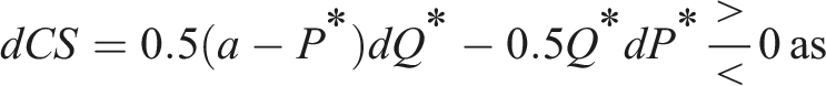

As equation (22) shows, the change in CS due to a pivot may be positive, zero, or even negative; in any event, it will be less positive than the change resulting from an outward shift of demand to the same new equilibrium. Moreover, if the pivot makes market demand more elastic than market supply (
New Producers and Producer Surplus
For a linear supply curve with 

Notice that an outward shift of the market supply curve implies
Consider three scenarios. First, if demand is perfectly elastic, so that 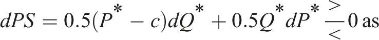

As equation (25) reveals, the effect on PS from additional sellers entering the market is positive so long as supply is less elastic than demand; when supply is more elastic than demand, a further counterclockwise pivoting of the market supply curve reduces PS (Miller, et al., 1988). In the limit, as m goes to infinity and the market supply curve approaches perfect elasticity, PS approaches zero; just as competition among producers pushes economic profit to zero, it can also eliminate producer surplus.
Market Adjustment to Long Run Equilibrium
Producer entry and exit provide the mechanism by which firms in competitive markets earn zero economic profits (
Summary of Differences Between Shifts and Pivots as Depictions of Market Entry by Homogeneous Agents. a
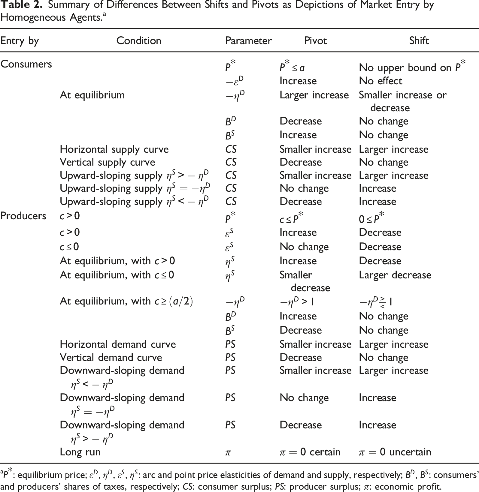
a
Nonlinear Functions
Linear supply and demand functions are certainly predominant in undergraduate textbooks and other pedagogical works. Indeed, the emphasis that most texts place on discussing the changing elasticity along a linear demand curve suggests the centrality of the linear form for educational purposes. And linear functions remain fairly common in empirical research, because linear regression techniques are often employed in estimation.
14
Even so, as a final caveat, we briefly consider alternative functional forms. Certainly, an isoelastic function behaves quite differently—by definition, it will not become more or less elastic as agents enter or exit the market. However, the isoelastic function is not only more complex to teach, it is also a rather special case: it is not clear that constant own-price elasticity generally applies to most consumers or most producers in most markets. Additionally, there are other nonlinear functional forms whose own-price elasticities will respond to market entry and exit. As one example, suppose the individual-level demand function is
Conclusion
With the exception of economics majors, most college students will only study economics at the principles level (Bosshardt & Walstad, 2017; Bosshardt and Watts, 2008). And although descriptions of the market are more detailed and comprehensive at the intermediate level, they are usually not fundamentally different from those taught earlier in introductory courses. Thus, the manner in which we portray economic models in these courses influences—one might say determines—the way that our students will think of the economy for the rest of their lives. It is imperative, therefore, that we provide simple but consistent and reasonably accurate models that describe reality as nearly as possible. The traditional practice of depicting entry or exit as shifting a linear market supply or demand curve is a convenient fiction, but it is unrealistic and inconsistent with the lesson regarding the construction of the market-level curve as a horizontal summation of individual agents’ curves. As a consequence, that practice also leads to erroneous conclusions regarding the effects of entry and exit on own-price elasticity, tax incidence, consumer surplus, producer surplus, and importantly, the competitive market adjustment to long run equilibrium. This paper therefore proposes that entry and exit be taught as pivoting the market supply and demand curves rather than shifting them.
Certainly, any pedagogical innovation must be presented in a manner that respects student abilities and time constraints in the course. Principles courses are already crowded with subject matter and there is an obvious opportunity cost to introducing new material. At that level, rather than treating market entry as a new topic, it can simply be noted as the logical conclusion to the customary demonstration of horizontal summation: entry flattens and exit steepens the market curve. The intuition can be stated as easily as in the classroom example above. Consequently, entry and exit can be included as factors affecting the elasticity of a market-level curve, and an even clearer distinction emerges naturally between these factors and those that change a market curve by altering individual curves. Any further analysis is more likely to be useful in an intermediate course, where students generally have greater interest in economic details and more familiarity with mathematics. There, the implications regarding consumer and producer surplus, tax incidence, and so forth can be explored as thoroughly as the instructor wishes. 15
Supplemental Material
Supplemental Material - Shift or Pivot? Market Entry and Exit With Linear Supply and Demand Curves
Supplemental Material for Shift or Pivot? Market Entry and Exit With Linear Supply and Demand Curves by Joseph G. Eisenhauer in The American Economist.
Footnotes
Acknowledgments
I thank participants at the 87th annual Midwest Economics Association conference, as well as this journal’s Associate Editor Laura Ahlstrom and an anonymous referee for helpful comments. Any errors are my own.
Declaration of Conflicting Interests
The author(s) declared no potential conflicts of interest with respect to the research, authorship, and/or publication of this article.
Funding
The author(s) received no financial support for the research, authorship, and/or publication of this article.
Supplemental Material
Supplemental material for this article is available online.
Notes
Author Biography
References
Supplementary Material
Please find the following supplemental material available below.
For Open Access articles published under a Creative Commons License, all supplemental material carries the same license as the article it is associated with.
For non-Open Access articles published, all supplemental material carries a non-exclusive license, and permission requests for re-use of supplemental material or any part of supplemental material shall be sent directly to the copyright owner as specified in the copyright notice associated with the article.