Using proxy data and vegetation modelling to predict past,current and future distributional shifts of Butea monosperma,a marker of land degradation in India

Abstract

Extensive deviations in spatio-temporal social and environmental dynamics currently alter the health of ecosystems and the services they provide. Detecting the causes that contribute to the distribution of a natural forest species capable of restoring the lost ecosystem function and productivity will aid in determining better food security, livelihoods and provision of ecosystem goods and services. We modelled the spatial range of Butea monosperma (B. monosperma) under past, that is, Last Glacial Maximum (LGM), Middle Holocene (MH), current and future (2070) climatic scenarios with Maximum Entropy (MaxEnt) trained on present-day occurrences. We identified areas of suitable habitats for which the estimation of habitat stability is predicted in all the models at different times. To validate the inferred suitable habitat, we tested the model by the current occurrence and fossil pollen data of B. monosperma. Our distribution models agree with the fossil pollen records for the MH (4,500–7,000 yr BP) and predict the prevalence of B. monosperma covering 84.22% of the Indian subcontinent with maximum habitat stability in western and southwestern India (10.95%). The widespread potential distribution of the plant species during the LGM supports the presence of the last remnants of tropical dry deciduous forest in the region. However, a decline in habitat suitability (62.84%) is predicted under current and future climatic scenarios with maximum stability (0.90%–3.09%) along the Western Ghats, Nilgiri hills, Gir range in the western India and north-eastern region covering the Assam Valley and foothills of Tripura and Mizo hills. Temperature seasonality (33.6%) measured in terms of variable contribution in MaxEnt model significantly affects the distribution shift of B. monosperma, along with annual precipitation (22.8%) and annual mean temperature (16.2%). Model results provide evidence of habitat reduction and identify the stability hotspots for B. monosperma for its conservation and establishment of land management policies mainly for the dry tropics.

Introduction

Global anthropogenic environmental change has led to serious impacts on species diversity, distribution and persistence in the last three decades, which in turn will act as a major cause of species loss shortly (Mishra et al., 2021; Pacifici et al., 2015). A substantial part (31%) of Earth’s land surface comprises a forest ecosystem (FAO & UNEP, 2020). Out of which a major part of the plant species in the world is from the tropical forests which cover only 7% of the Earth’s surface. These tropical forests are wrecked by anthropogenic activities (Morris, 2010), leading to forest degradation clearing nearly 85% of the tree species (Baboo et al., 2017; Kittur et al., 2014; Tiwari et al., 2021). The rate of loss of species due to human activities is 3–8 times higher than natural disturbances leading to habitat alterations (Costanza et al., 1997; Karki et al., 2017). The tropical biome has the highest rate of forest destruction and degradation among the four global climate domains viz. tropical, subtropical, temperate and boreal (Hansen et al., 2013).

One such economically and ecologically significant tree species in a forest ecosystem is Butea monosperma forming dominant covers in the moist/dry deciduous forests throughout the Indian subcontinent (Khan, 2010). B. monosperma is one such dry deciduous tree species of the family Fabaceae, which is native to the tropical and subtropical environment of the Indian subcontinent and all Asian hemispheres (Sutariya & Saraf, 2015). B. monosperma is a distinctive tree species of plains, generally found in small patches along cultivated fields, pastures and open grasslands, escaping extinction due to its ability to resist and reproduce from root suckers and seeds (Orwa et al., 2009). B. monosperma has a great potential to restore and enhance biological activities in degraded lands through nitrogen fixation and promote vegetation establishment (Rai et al., 2016). Although found in several parts of India and Southeast Asia still the plant is under pressure due to climate variation and human disturbances (Burli & Khade, 2007). B. monosperma is selected as a target species, as it is an adaptable tree species in the subtropical areas that requires alkaline, badly drained swampy soils, sunny areas and an optimal rainfall of 500 to 2,500 mm (Fageria & Rao, 2015). The plant regenerates naturally in mixed deciduous forests and is greatly exploited for fuelwood and several other domestic purposes (Sridhar et al., 2016). It generally grows up to an elevation of 1,200 m excluding very arid regions (Khare, 2007). B. monosperma has environmental and ecological functions related to land rehabilitation through nitrogen fixation, carbon sequestration in soil, water conservation and controlling soil erosion (Kumari et al., 2005). Overexploitation of its resources combined with expansion and development has caused a drop in the surviving population of B. monosperma, which makes it an ideal investment or choice for planning restoration measures. B. monosperma grows all along the Indian peninsula forming patches of forest, from the southwestern Ghats to the Indo-Gangetic plains (Chopra et al., 1958; Fageria & Rao, 2015; Vashishtha et al., 2013). It is one of the associates of Sal forests (Shorea robusta) in the salt belts, along with Dalbergia-Anogeissus-Helicteres in the deciduous forests, and with Pongamia pinnata along the river channels and streams (Lohot et al., 2016).

Climate change is the main driving feature in these regions for rising temperatures and changing precipitation patterns (Loo et al., 2015; Sivakumar & Stefanski, 2011). In the past 100 years, global warming and land-use changes have caused substantial variation in the spatiotemporal environmental patterns (Benito et al., 2009; Hughes, 2000) and these changes, in turn, cause a major threat to biodiversity and conservation of forest ecosystem through habitat depletion and changes in plant species composition (Hughes, 2000; Sala et al., 2001; Walther et al., 2002). Fossil pollen records from the Indian subcontinent suggested that between ~18,658 and 7,340 cal yr BP, the open vegetation chiefly comprises of grasses (Poaceae), Tubuliflorae (Asteroideae; Asteraceae family), together with sparsely distributed tree taxa, such as Madhuca indica, members of Sapotaceae, Syzygium, Schleichera, Holoptelea, Lannea coromandelica, Lagerstroemia and Adina under a cool and dry climate with reduced monsoonal rainfall, which globally matches with the Last Glacial Maximum (LGM) (Quamar & Bera, 2020). However, Trivedi et al. (2019) suggested an open grassland type of vegetation mainly containing herbs and sparse pollen of Holoptelea integrifolia, as well as ruderal plants, such as Amaranthaceae, Brassicaceae, Artemisia and Caryophyllaceae members along the central Ganga Plain, India between ~25,500 and 22,200 cal yr BP. During Middle Holocene (MH), between 7,150 and 4,657 yr BP, open mixed tropical deciduous forests existed in central India with the dominance of Madhuca indica, Acacia (cf. A. nilotica) and members of Sapotaceae, along with S. robusta and Symplocos under a warm and moderately humid climate with strengthened monsoon condition (Quamar & Chauhan, 2012). Globally, it corresponds to the Holocene Climatic Optimum (HCO), which falls broadly within the time interval of 7,000–4,000 BP (Benarde, 1992). However, Chauhan and Quamar (2012) suggested dense mixed moist tropical deciduous forests between 5,409 and 4,011 years BP with the increased appearance of the prominent moist elements, such as Terminalia, Madhuca indica, Grewia and Schleichera oleosa and dry forest elements, such as Lannea coromandelica, Emblica officinalis, Aegle marmelos and Bombax ceiba with sporadic presence of S. robusta, Holoptelea and Ehretia laevis in central India during the HCO. Chauhan and Quamar (2012) suggested that between 6,000 and 5,409 years BP, the area supported open mixed moist tropical deciduous forests largely comprised Lannea coromandelica, Terminalia, Madhuca indica, Grewia, Schleichera oleosa, Syzygium and Aegle marmelos, along with the scanty presence of Lannea parviflora, Madhuca parvifolia, Haldina cordifolia, Acacia, Bombax ceiba, Emblica officinalis and B. monosperma together with a few thickets of Acanthaceae (cf. Rungia), Petalidium, Peristrophe and Strobilanthes in open areas interspersed with the forest stands under a warm and relatively less humid climate with reduced monsoon rainfall.

The potential effect of anthropogenic climate change on the species distribution can be effectively assessed through species distribution models (SDMs), using current climatic conditions and species occurrence data to model the realised niche of the plant species (Hutchinson, 1957). Species distribution modelling is a numerical tool for characterising the statistical relationship between the species occurrence and environmental variables (Elith & Leathwick, 2009; Guillera-Arroita et al., 2015; Guisan & Zimmermann, 2000). SDMs are broadly used in biogeography studies to signify the ecological niches of plants and animals and to forecast the geographical distribution of habitats (Taleshi et al., 2019). These distribution models are further projected in geographic space by using estimations of past and future climatic patterns (Varela et al., 2011). Understanding how climatic changes affect the plant species distribution is essential for studying biogeography and developing conservation strategies (Ribeiro et al., 2019). Evaluating potential distribution for different periods (past and future time scenarios) using ecological parameters projected with present occurrence information (Alvarado-Serrano & Knowles, 2014). The Maximum Entropy (MaxEnt) SDM is a bioclimatic model that uses presence-only data, finding that absence data are hardly found or consistent and evaluates the distribution of a species depending on climatic controls (Deb et al., 2017; Phillips et al., 2006) and has performed well among various modelling approaches (Elith et al., 2006; Ortega-Huerta & Peterson, 2008).

In the present study, the suitable habitat zone for B. monosperma was modelled under the past (LGM and MH), current and future (the 2070s) climatic scenarios using Maxent modelling. The model uses species presence records and current climatic variables, such as precipitation, temperature, altitude and aspect to detect the best suitable distribution of the plant species across the Indian subcontinent. The mid-Holocene model projection for the targeted species is further cross-validated by fossil pollen evidence of the species from various palaeovegetation reconstruction studies. This has considerable potential to bridge the gaps between paleoecology and species distribution modelling by integrating palynological analysis that spans the LGM and MH and climate modelling that highlights the spatial context for range contraction/expansion and migration. It is hypothesised that if the climatic condition and anthropogenic pressure on B. monosperma are not controlled and monitored in India then it would lead to a significant decrease in the suitable habitat of this indispensable tree species soon from various parts of the subcontinent (Tiwari et al., 2021). Consequently, it is essential to hindcast the distribution of the target species B. monosperma to trace its distribution in past climatic conditions (paleoSDM) and thereby precisely classify the suitable habitats for B. monosperma under the extant and future (the 2070s) climate change scenarios (neoSDM) for its restoration and conservation management (Graham et al., 2004). Predicted climate change effects on B. monosperma distribution will help in designing proactive management strategies, bearing in mind the major ecosystem-level feedback from the model.

Materials and Methods

Species Occurrence Data

Species occurrence points, an essential tool to map the probability distribution of any species, are the geographical coordinates of the species. To predict the suitable habitat of our targeted species, that is, B. monosperma, we compiled both primary and secondary occurrence data from different sources. The primary data points were obtained through a field survey using Garmin GPS around the states of Madhya Pradesh, Chhattisgarh, Uttar Pradesh, Maharashtra and Rajasthan. Similarly, the secondary data points were extracted from the Global Biodiversity Information Facility (GBIF) database (GBIF, 2022), Indian Biodiversity Portal (IBP, 2022) and published literature. From the above-mentioned sources, 663 occurrence points of the species were obtained, and their coordinates were extracted and recorded for use in the model. Spatial sampling bias is an issue in predictive modelling because it leads to spatially auto-correlated occurrences, lowering model accuracy (Boria et al., 2014). All occurrence points were filtered at 1 km × 1 km using the ArcGIS SDM toolbox in ArcGIS 10.5 software to solve this problem. Finally, a total of 296 presence records of B. monosperma were obtained for constructing the models (Supplementary File No. 1).

Environmental Variables

To model the potential distribution of B. monosperma, we retrieved the current climatic variables from WorldClim database (http://www.worldclim.org), version 1.4 (Hijmans et al., 2005). This climatic data covers the information of minimum, maximum and mean values of monthly, quarterly and annual precipitation and temperatures for 1960–1990. In addition, two topographic variables, altitude and aspect were used as additional predictor variables. For future climatic projections, we used data from the Hadley Global Environment Model 2-Earth System (HADGEM2-ES) of the fifth assessment report (AR5) of the Intergovernmental Panel for Climate Change (Moss et al., 2010), which represents simulations for the Representative Concentration Pathways such as RCP 2.6, RCP 4.5, RCP 6.0 and RCP 8.5 where the number refers to the radiative forcing measured in watts per square meter (Wm-2) (Van Vuuren et al., 2011) for 2070 time span. In addition, we extracted past bioclimatic data for the LGM (ca. 22,000 years ago) and MH (ca. 6,000 years ago) from the original simulations of General Circulation Models (GCMs) built on HadGEM2-ES from CMIP5 (Coupled Model Intercomparison Project) (Gent et al., 2011). All the selected variables for past, current and future had a spatial resolution of 30 arc seconds, ~1 × 1 km except LGM (2.5 min, ~5 × 5 km), which helps in the proper planning of conservation strategies.

Four RCPs were selected for species distribution modelling of B. monosperma, which describe different future climate scenarios depending on the amount of greenhouse gases emitted in the coming years (IPCC, 2013; Moss et al., 2008). According to RCP 2.6, global annual greenhouse gas emissions will be highest during 2010–2020 and decline substantially (Meinshausen et al., 2011). On the other hand, RCP 4.5 is a positive scenario where emission is predicted to peak around 2040 and then decline (Bernie, 2010). RCP 6.0 is a transitional scenario where the assumption is that total radiative forcing has been alleviated by 2010 by adapting various technologies and strategies to reduce emissions in the future. In the case of RCP 8.5, it is predicted that an uncontrolled increase in greenhouse gas emissions will be seen throughout the twenty-first century (Riahi et al., 2011).

Selection of Bioclimatic Predictors

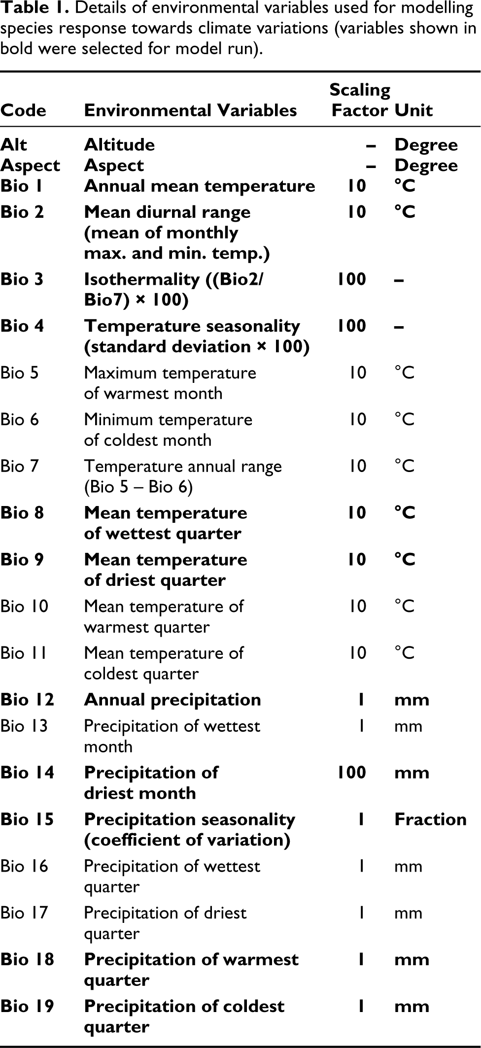
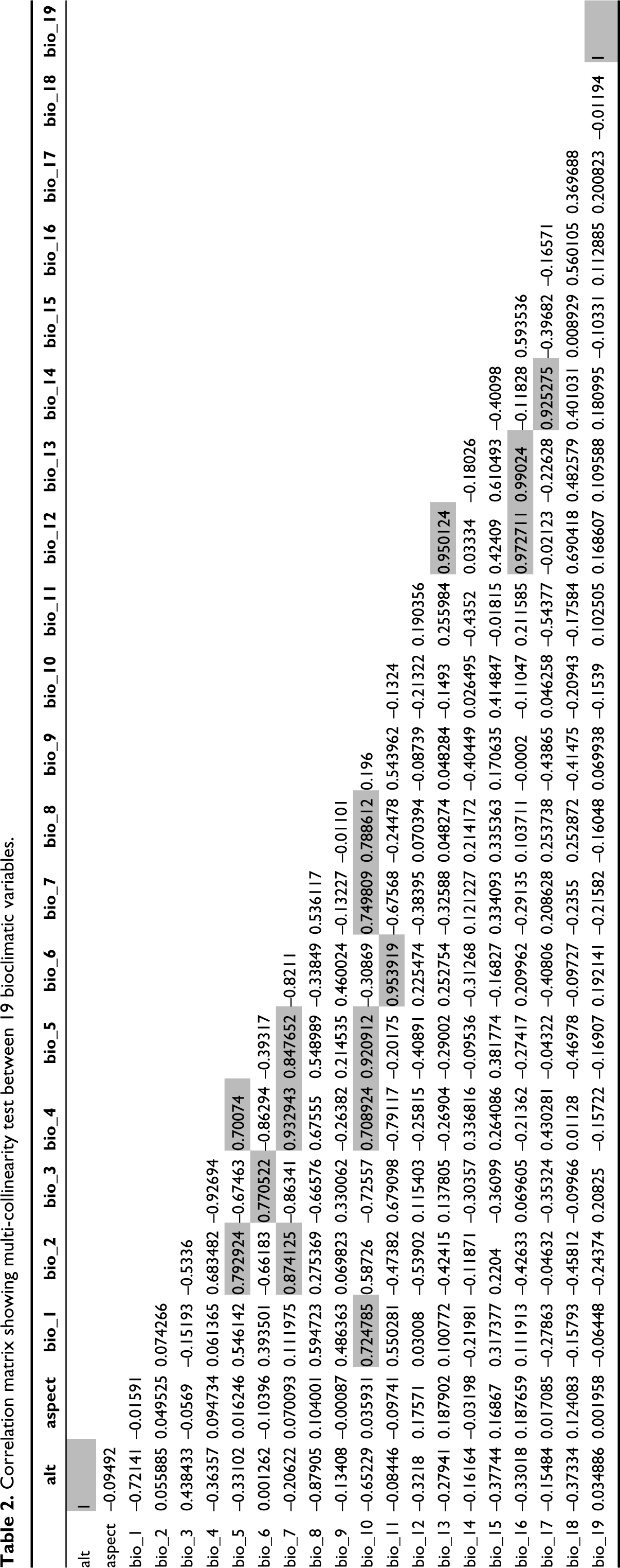
SDMs work on the relationship between the species occurrence data and climate factors. Input bioclimatic factors are spatially auto-correlated hence the actual relationships may not emerge thus different combinations of bioclimatic variables can project species distribution with equal efficiency. The correlation of these bioclimatic variables leads to weak model performance with distorted analyses (Dormann et al., 2013). Hence, multi-collinearity tests are essential through Pearson’s correlation to observe associations between factors. Highly correlated bioclimatic factors having a correlation coefficient r > 0.7 were omitted in the final analysis (Yang et al., 2013) (Table 2). In total, 11 bioclimatic factors from a total of nineteen factors were retained to model B. monosperma distribution. These include temperature seasonality (BIO4), annual precipitation (BIO12), annual mean temperature (BIO1), precipitation seasonality (BIO15), precipitation of coldest quarter (BIO19), mean temperature of driest quarter (BIO9), isothermality (BIO3), precipitation of driest month (BIO14), mean diurnal range (BIO2), mean temperature of wettest quarter (BIO8), and precipitation of warmest quarter (BIO18) and two topographic variables altitude and aspect (Table 1).

Table 1.

Details of environmental variables used for modelling species response towards climate variations (variables shown in bold were selected for model run).

Code	Environmental Variables	Scaling Factor	Unit
Alt Aspect Bio 1	Altitude Aspect Annual mean temperature	––10	Degree Degree °C
Bio 2	Mean diurnal range (mean of monthly max. and min. temp.)	10	°C
Bio 3	Isothermality ((Bio2/Bio7) × 100)	100	–
Bio 4	Temperature seasonality (standard deviation × 100)	100	–
Bio 5	Maximum temperature of warmest month	10	°C
Bio 6	Minimum temperature of coldest month	10	°C
Bio 7	Temperature annual range (Bio 5 – Bio 6)	10	°C
Bio 8	Mean temperature of wettest quarter	10	°C
Bio 9	Mean temperature of driest quarter	10	°C
Bio 10	Mean temperature of warmest quarter	10	°C
Bio 11	Mean temperature of coldest quarter	10	°C
Bio 12	Annual precipitation	1	mm
Bio 13	Precipitation of wettest month	1	mm
Bio 14	Precipitation of driest month	100	mm
Bio 15	Precipitation seasonality (coefficient of variation)	1	Fraction
Bio 16	Precipitation of wettest quarter	1	mm
Bio 17	Precipitation of driest quarter	1	mm
Bio 18	Precipitation of warmest quarter	1	mm
Bio 19	Precipitation of coldest quarter	1	mm

Table 2.

Correlation matrix showing multi-collinearity test between 19 bioclimatic variables.

	alt	aspect	bio_1	bio_2	bio_3	bio_4	bio_5	bio_6	bio_7	bio_8	bio_9	bio_10	bio_11	bio_12	bio_13	bio_14	bio_15	bio_16	bio_17	bio_18	bio_19
alt	1
aspect	–0.09492
bio_1	–0.72141	–0.01591
bio_2	0.055885	0.049525	0.074266
bio_3	0.438433	–0.0569	–0.15193	–0.5336
bio_4	–0.36357	0.094734	0.061365	0.683482	–0.92694
bio_5	–0.33102	0.016246	0.546142	0.792924	–0.67463	0.70074
bio_6	0.001262	–0.10396	0.393501	–0.66183	0.770522	–0.86294	–0.39317
bio_7	–0.20622	0.070093	0.111975	0.874125	–0.86341	0.932943	0.847652	–0.8211
bio_8	–0.87905	0.104001	0.594723	0.275369	–0.66576	0.67555	0.548989	–0.33849	0.536117
bio_9	–0.13408	–0.00087	0.486363	0.069823	0.330062	–0.26382	0.214535	0.460024	–0.13227	–0.01101
bio_10	–0.65229	0.035931	0.724785	0.58726	–0.72557	0.708924	0.920912	–0.30869	0.749809	0.788612	0.196
bio_11	–0.08446	–0.09741	0.550281	–0.47382	0.679098	–0.79117	–0.20175	0.953919	–0.67568	–0.24478	0.543962	–0.1324
bio_12	–0.3218	0.17571	0.03008	–0.53902	0.115403	–0.25815	–0.40891	0.225474	–0.38395	0.070394	–0.08739	–0.21322	0.190356
bio_13	–0.27941	0.187902	0.100772	–0.42415	0.137805	–0.26904	–0.29002	0.252754	–0.32588	0.048274	0.048284	–0.1493	0.255984	0.950124
bio_14	–0.16164	–0.03198	–0.21981	–0.11871	–0.30357	0.336816	–0.09536	–0.31268	0.121227	0.214172	–0.40449	0.026495	–0.4352	0.03334	–0.18026
bio_15	–0.37744	0.16867	0.317377	0.2204	–0.36099	0.264086	0.381774	–0.16827	0.334093	0.335363	0.170635	0.414847	–0.01815	0.42409	0.610493	–0.40098
bio_16	–0.33018	0.187659	0.111913	–0.42633	0.069605	–0.21362	–0.27417	0.209962	–0.29135	0.103711	–0.0002	–0.11047	0.211585	0.972711	0.99024	–0.11828	0.593536
bio_17	–0.15484	0.017085	–0.27863	–0.04632	–0.35324	0.430281	–0.04322	–0.40806	0.208628	0.253738	–0.43865	0.046258	–0.54377	–0.02123	–0.22628	0.925275	–0.39682	–0.16571
bio_18	–0.37334	0.124083	–0.15793	–0.45812	–0.09966	0.01128	–0.46978	–0.09727	–0.2355	0.252872	–0.41475	–0.20943	–0.17584	0.690418	0.482579	0.401031	0.008929	0.560105	0.369688
bio_19	0.034886	0.001958	–0.06448	–0.24374	0.20825	–0.15722	–0.16907	0.192141	–0.21582	–0.16048	0.069938	–0.1539	0.102505	0.168607	0.109588	0.180995	–0.10331	0.112885	0.200823	–0.01194	1

Model Description

We modelled the potentially suitable habitat for B. monosperma using the Maxent Niche model version 3.4.1. (Phillips et al., 2006). The MaxEnt Model performs very well in comparison to other methods developed for predicting species distributions, using presence-only data (Bosso et al., 2016; Elith et al., 2006). Its output is based on the likelihood distribution of a species occurrence (Elith et al., 2011). The model was calibrated for the current climate and projected for past and future climatic scenarios. In total, 75% of the total occurrence points were selected at random as training data, and the remaining 25% was used as test data with independent validation. In total, 10 replicates of the model were run with 5,000 iterations. Model validation was performed using a subsampling strategy. To test the evenness of the variable curves, the default regularisation multiplier equal to 1 was used. Additionally, the following process was performed (1) random seed for each iteration; (2) removal of duplicate occurrence records; (3) plotting of data; (4) append summary results to MaxEnt results in csv format; (5) maximum iterations = 5,000; (6) write background predictions. The rest of the settings were set to default. We created the cloglog MaxEnt output (complementary log-log) to estimate the probability of species presence (Phillips et al., 2017).

Figure 1.

The present distribution points of B. monosperma in the Indian subcontinent.

Results and Discussion

Major Bioclimatic Factors Driving the Distribution of B. monosperma

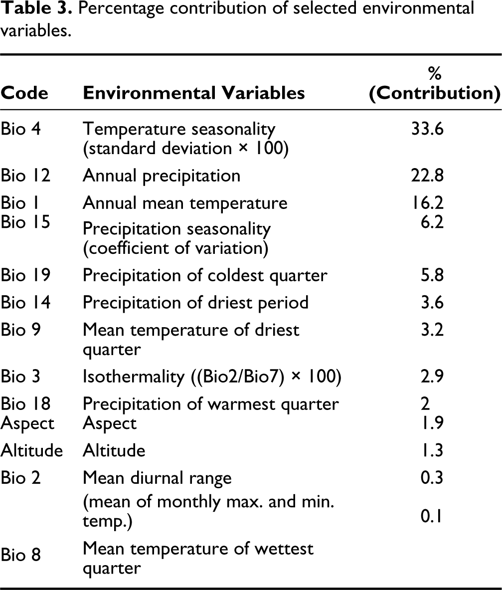
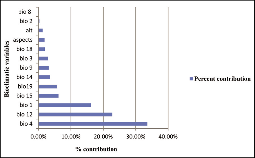
The MaxEnt results revealed that temperature seasonality and annual precipitation were the main limiting bioclimatic factors on the distribution of B. monosperma (Table 3). In addition, these results also depict the highest contribution of temperature seasonality (BIO4, 33.6%), annual precipitation (BIO12, 22.8%), mean annual temperature (BIO1, 16.2%) and precipitation seasonality (BIO15, 6.2%) on B. monosperma distribution, which appeared in all 10 model replicates. However, aspect (Aspect, 1.98%), altitude (Alt, 1.3%), the mean diurnal range (Mean of monthly max. and min. Temp [BIO2, 0.3%]) and mean temperature of the wettest quarter (BIO8, 0.1%), contributed the least (Table 3) (Figure 2). Based on our present study, we inferred that climate potentially affects the distribution of B. monosperma across the Indian subcontinent. Our result is closely in agreement with the previously published article (Tiwari et al., 2021) where the distribution of B. monosperma was influenced by temperature and precipitation. According to the Agroforestry Database 4.0, the climatic requirements of B. monosperma state that it can grow at a mean annual temperature of 4–49°C (Orwa et al., 2009). Again, Fageria and Rao (2015) have reported that the growth of B. monosperma occurs best at an elevation of 1,200 m a.s.l. along with an ideal rainfall of 500–2,500 mm.

Table 3.

Percentage contribution of selected environmental variables.

Code	Environmental Variables	% (Contribution)
Bio 4	Temperature seasonality (standard deviation × 100)	33.6
Bio 12	Annual precipitation	22.8
Bio 1Bio 15	Annual mean temperaturePrecipitation seasonality (coefficient of variation)	16.26.2
Bio 19	Precipitation of coldest quarter	5.8
Bio 14	Precipitation of driest period	3.6
Bio 9	Mean temperature of driest quarter	3.2
Bio 3	Isothermality ((Bio2/Bio7) × 100)	2.9
Bio 18Aspect	Precipitation of warmest quarterAspect	21.9
Altitude	Altitude	1.3
Bio 2Bio 8	Mean diurnal range(mean of monthly max. and min. temp.)Mean temperature of wettest quarter	0.30.1

Figure 2.

Percentage contribution of selected environmental variables.

Model Accuracy

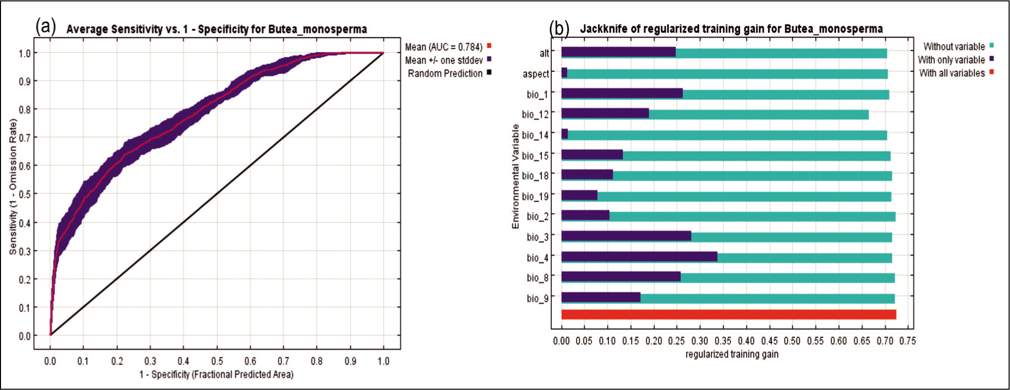
The generated models were weighed through the area under the curve (AUC) for receiver operating characteristic (ROC) plot statistics (Swets, 1988). The predictive accuracies of the model were significant for B. monosperma with an AUC value of 0.784 (Figure 4a). AUC values of 0.5–0.7 specify poor model performance, 0.7–0.9 specify good model performance and >0.9 denote outstanding model performance (Swets, 1988). According to the criteria of Swets (1988), the accuracy of MaxEnt models for B. monosperma, based on their AUC value (0.784), indicated a good model performance (Figure 4a).

Figure 3.

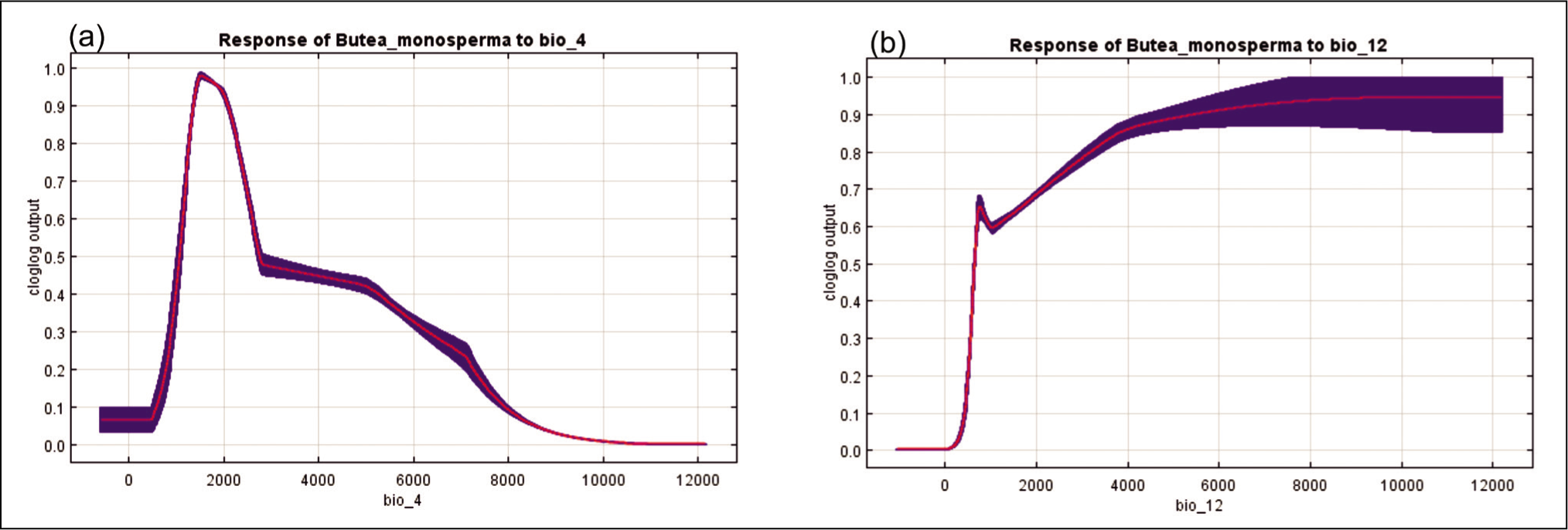
Relationship between selected Bioclimatic predictors and probability of species suitability of B. monosperma (a) BIO4 and (b) BIO12.

Figure 4.

(a) Represents the results of the AUC (area under ROC) curves in developing B. monosperma habitat suitability model; (b) Represents the results of the Jackknife test of variables’ contribution in modeling B. monosperma habitat suitability distribution.

In addition to AUC, we used true skill statistic (TSS) and Kappa methods to test model performance. The TSS and Kappa values for the studied model were estimated as 0.723 and 0.713 respectively. The TSS (Allouche et al., 2006) calculates a threshold-dependent statistical matrix with value ranges of 1 to +1 to measure model accuracy. TSS values of >0.8 indicate good to excellent performance, 0.6–0.8 indicate useful and 0.2–0.5 indicate poor performance (Coetzee et al., 2009; Gama et al., 2017; Shabani et al., 2016). Cohen (1960) proposed interpreting the Kappa result as follows: 0 as no agreement, 0.01–0.20 as none to slight, 0.21–0.40 as fair, 0.41–0.60 as moderate, 0.61–0.80 as substantial and 0.81–1.00 as almost perfect agreement. The estimated TSS = 0.723 and Kappa (Kp) = 0.713 values are also suggestive of a useful and substantial model performance respectively.

Jackknife Test and Response Curves

The Jackknife test calculated the impact of each bioclimatic variable on the model (Figure 4b). Temperature seasonality had the best information, with the highest contribution. The response curves produced by the MaxEnt model showed how the logistic prediction of B. monosperma distribution varies with changes in the predictive variables, keeping all other environmental variables at the average sample points. According to the response curve, a 0.6 probability of B. monosperma existence was observed with the temperature change of 17–22% coefficient of variation (CV) over the year (temperature seasonality) (Figure 3a). Again, the probability of suitable habitat for B. monosperma remained high in those areas where annual precipitation ranged from 800 to 2,100 mm (Figure 3b).

Current Distribution of B. monosperma in India

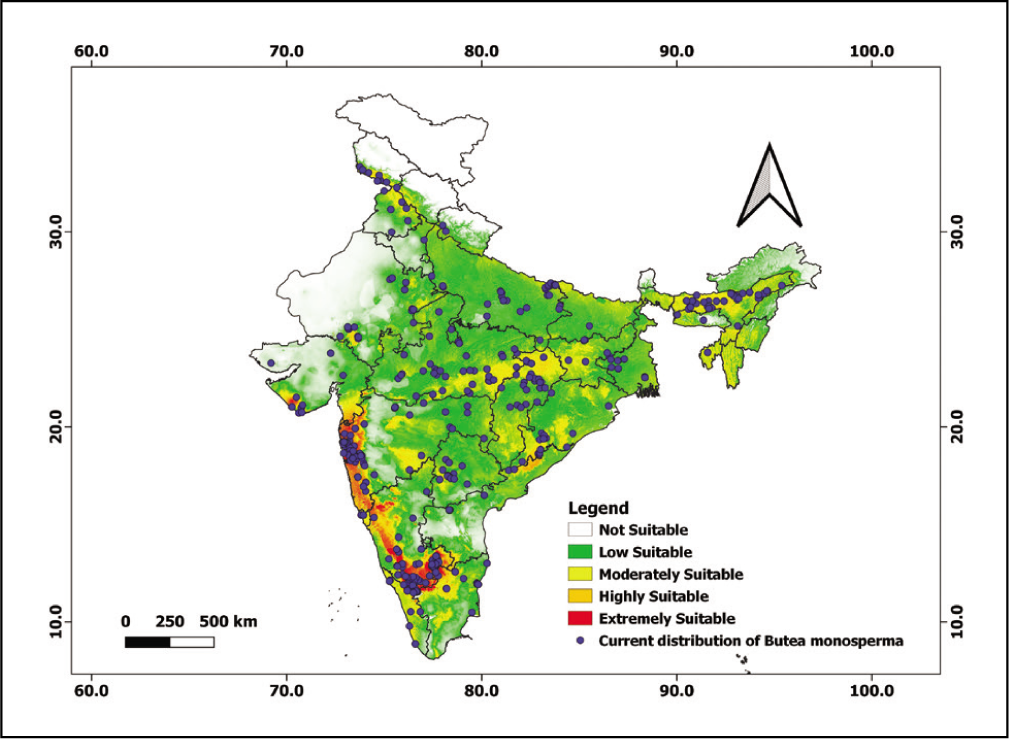
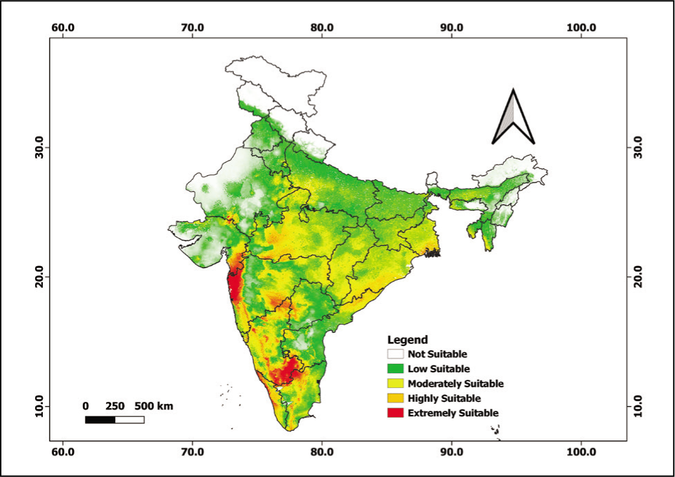
Model results combining current climate and species occurrence points predicted that western India covering the Gir range in Gujrat, the Western Ghats and the Nilgiri hills are extremely suitable habitats (red, 117184.84 sq. km) for B. monosperma. However, the north-eastern region mainly covers the Assam Valley and foothills of Tripura and Mizo hills, Vembanad wetland in Kerala, foothills of Sahyadris, Girnar and Barda hills in western India, also Vindhya range, Mahadeo hills and Ramgarh hills in central India region are highly and moderately suitable (orange; 159165.94 sq. km and yellow; 636154.63 sq. km) for B. monosperma distribution. Almost all the states of the Indian subcontinent possess low suitable habitat (green, 1472644.23 sq. km) for B. monosperma except the Great Indian Thar desert in Rajasthan, Srinagar and Ladakh region in northern India (Figures 1 and 6) (Table 4).

Figure 5.

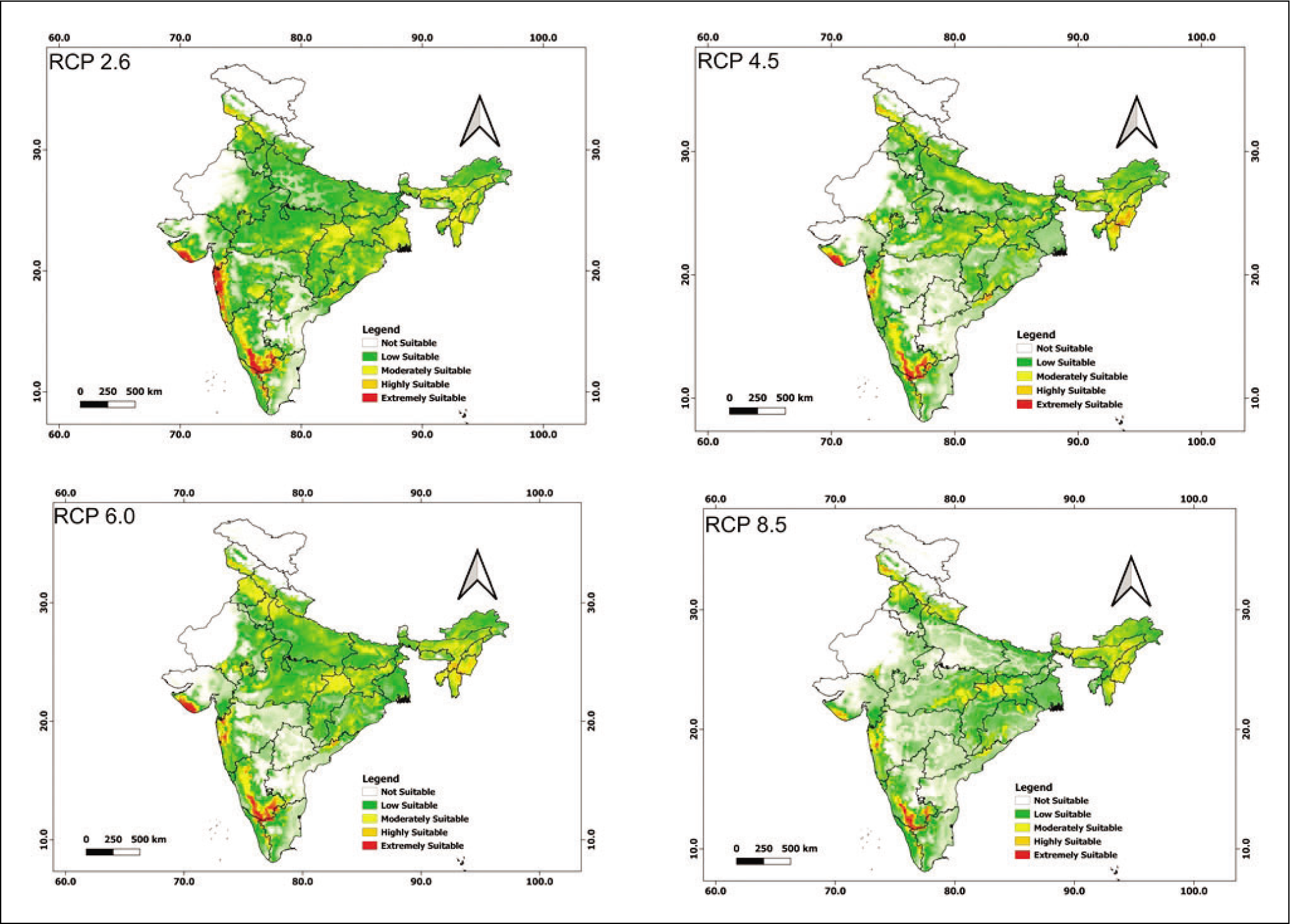
(a) Predicted future distribution model of B. monosperma in 2070s under RCP 2.6; (b) Predicted future distribution model of B. monosperma in 2070s under RCP 4.5; (c) Predicted future distribution model of B. monosperma in 2070s under RCP 6.0; (d) Predicted future distribution model of B. monosperma in 2070s under RCP 8.5.

Figure 6.

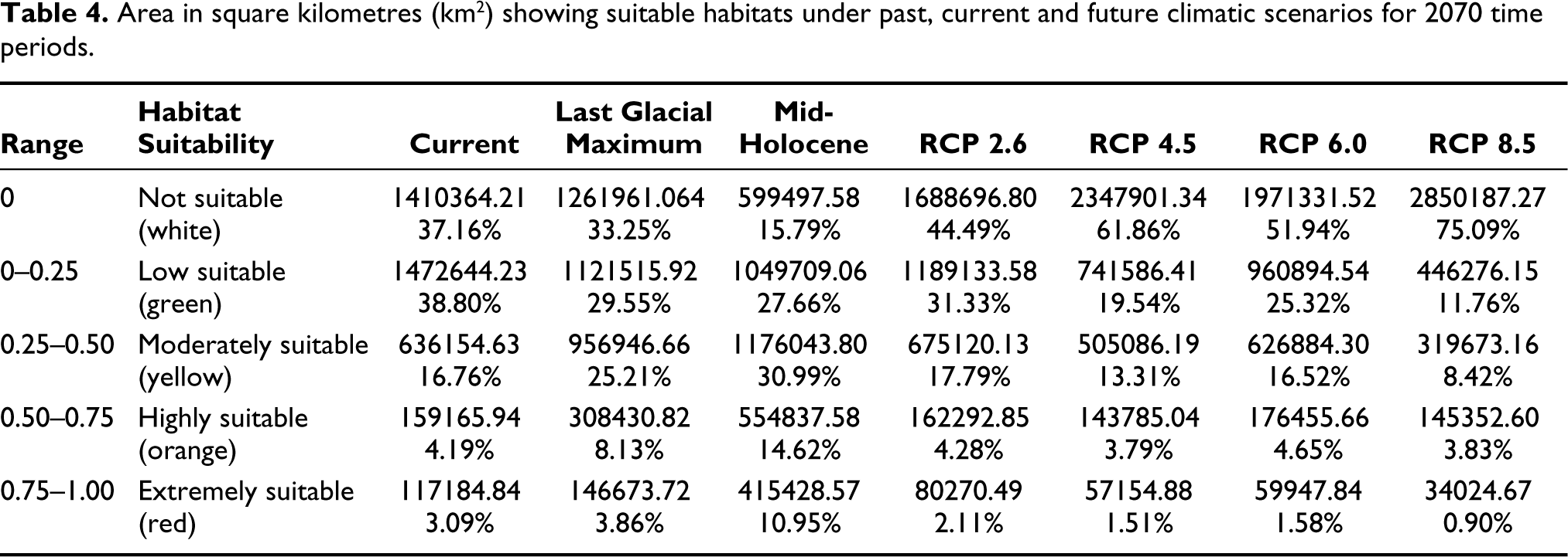
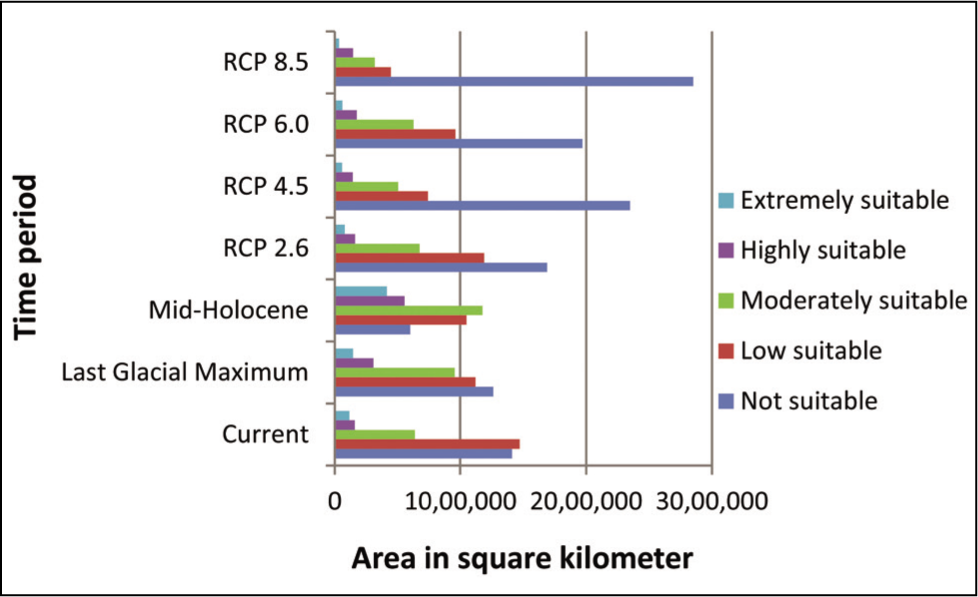
Area in square kilometres (km²) showing suitable habitats under past, current and future climatic scenarios for 2070 time periods.

Table 4.

Area in square kilometres (km²) showing suitable habitats under past, current and future climatic scenarios for 2070 time periods.

Range	Habitat Suitability	Current	Last Glacial Maximum	Mid-Holocene	RCP 2.6	RCP 4.5	RCP 6.0	RCP 8.5
0	Not suitable(white)	1410364.2137.16%	1261961.06433.25%	599497.5815.79%	1688696.8044.49%	2347901.3461.86%	1971331.5251.94%	2850187.2775.09%
0–0.25	Low suitable(green)	1472644.2338.80%	1121515.9229.55%	1049709.0627.66%	1189133.5831.33%	741586.4119.54%	960894.5425.32%	446276.1511.76%
0.25–0.50	Moderately suitable(yellow)	636154.6316.76%	956946.6625.21%	1176043.8030.99%	675120.1317.79%	505086.1913.31%	626884.3016.52%	319673.168.42%
0.50–0.75	Highly suitable(orange)	159165.944.19%	308430.828.13%	554837.5814.62%	162292.854.28%	143785.043.79%	176455.664.65%	145352.603.83%
0.75–1.00	Extremely suitable (red)	117184.843.09%	146673.723.86%	415428.5710.95%	80270.492.11%	57154.881.51%	59947.841.58%	34024.670.90%

The distribution range is in confirmation with the distribution pattern reported in several studies of B. monosperma (Burli & Khade, 2007; Chandraker, 2014; Chopra et al., 1958; Mazumder et al., 2011; Sridhar et al., 2016; Sutariya & Saraf, 2015). In southwestern India, an extremely suitable habitat was found in the Western Ghats covering states like Maharashtra, Karnataka and Nilgiri hills, which are in agreement with the distribution pattern reported in numerous articles on B. monosperma (Fageria & Rao, 2015; Vashishtha et al., 2013). Similarly, the most conducive habitat of B. monosperma was found in Peninsular India, which agrees well with the distribution reported by Vashishtha et al. (2013) and Chandraker (2014). Mahajan and Kale (2006) have documented the distribution of B. monosperma in the north-western part of India as community plants and other tree species.

Distribution of B. monosperma in Future Climate Scenarios

Under future climatic scenario RCP 2.6 (2070), extremely suitable habitat will sustain in the Gir range in Gujarat, Western Ghats and Nilgiri hills; however, it will only diminish in Uttara Kannada and Shimoga regions of Karnataka compared to current climatic scenarios. The highly and moderately suitable habitat of B. monosperma will be present in the north-eastern region mainly the Assam Valley, foothills of Tripura, Barail range and Mizo hills, Western Ghats, foothills of Sahyadris, Girnar and Barda hills in western India, also Vindhya range, Mahadeo hills and Ramgarh hills in central India. Interestingly, low suitable habitat will convert into moderately suitable habitat in West Bengal state under RCP 2.6. Furthermore, the low suitable habitats will decrease in some regions of Telangana, Andhra Pradesh and Tamil Nadu (Figure 5a). Under RCP 4.5 and RCP 6.0 (2070), the model shows a significant decline in the extremely suitable habitat of B. monosperma in the Western Ghats regions, it will only be present in Satmala range in Maharashtra, Nilgiri hills in southern India and Gir range in western India while in the north-eastern region, it will only exist in Barail range, Mizo and Naga hills. Furthermore, the low suitable habitat will considerably reduce in some regions of Maharashtra, Telangana, Andhra Pradesh and Tamil Nadu state. However, it will withstand in central India and the north-eastern region (Figure 5b and c). Under RCP 8.5 (2070), the model predicted that the habitat suitability would severely decline and showed a very low distribution in the Gir range in western India and the Satmala range in Maharashtra. However, it will be positively sustained in Nilgiri hills in southern India. The moderately and low suitable habitats will be preserved in the north-eastern and central India region, respectively (Figure 5d).

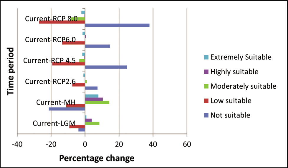
Our analysis also revealed that by 2070, there would be a decrease in extremely suitable habitat from the current scenario by 0.97%, 1.58%, 1.51% and 2.19%, low suitable habitat by 7.47%, 19.26%, 13.48% and 27.04% in all future climatic scenarios, that is, RCP 2.6, 4.5, 6.0 and 8.5 respectively. This led to an increase in unsuitable areas by 7.33%, 24.70%, 14.78% and 37.93% for all RCP 2.6, RCP 4.5, RCP 6.0 and RCP 8.5 respectively. However, the analysis showed a significant increase during the LGM and MH in extremely suitable habitats by 0.78 and 7.86% and low suitable habitats by 9.25% and 11.14%, respectively, compared to the current scenario. Again, the not suitable habitat showed a decrease by 3.91% and 21.36% for the LGM and MH, respectively (Table 5; Figure 7).

Table 5.

Percentage change in suitable habitat area in future scenario 2070.

Range	Habitat Suitability	Current-LGM (%)	Current-MH(%)	Current-RCP 2.6 (%)	Current-RCP 4.5 (%)	Current-RCP 6.0 (%)	Current-RCP 8.5 (%)
0	Not suitable(white)	–3.91	–21.36	7.33	24.70	14.78	37.93
0–0.25	Low suitable(green)	–9.25	–11.14	–7.47	–19.26	–13.48	–27.04
0.25–0.50	Moderately suitable(yellow)	8.45	14.22	1.03	–3.45	–0.24	–8.34
0.50–0.75	Highly suitable(orange)	3.93	10.42	0.08	–0.41	0.46	–0.36
0.75–1	Extremely suitable(red)	0.78	7.86	–0.97	–1.58	–1.51	–2.19

Figure 7.

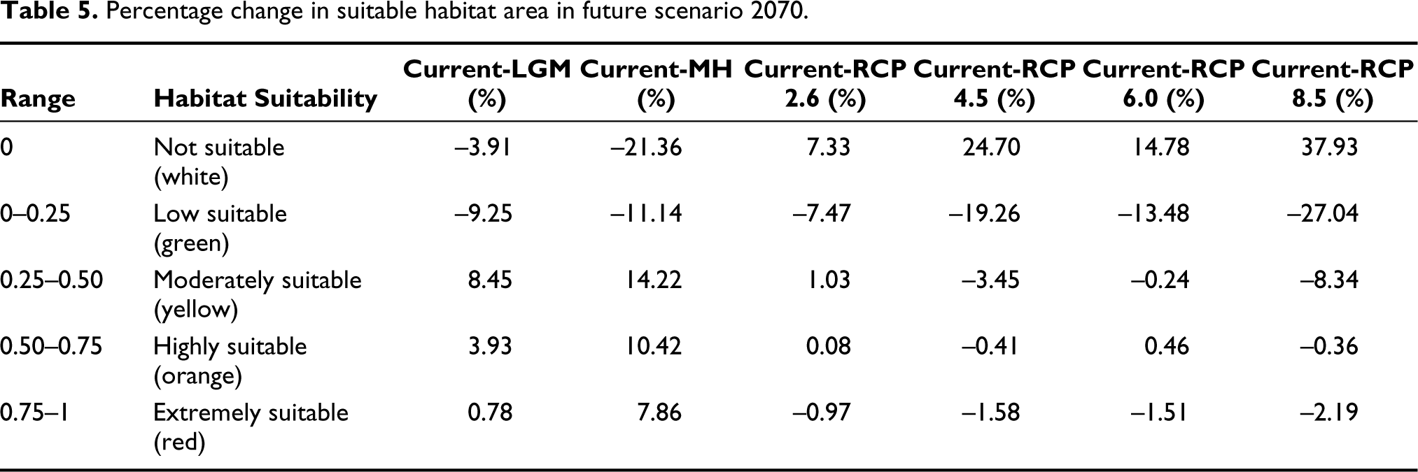
Percentage change in suitable habitat area in future scenario 2070.

In the future climatic scenarios, our result suggested that the habitat suitability range of B. monosperma is going to decrease (Figure 5a–d). There would be a severe decline in the extremely suitable habitat for B. monosperma in Western Ghats regions; however, it will considerably be sustained in the Nilgiri hills in southern India. According to regional studies, the dry deciduous forests of the Western Ghats may decline as a result of projected climate change (Sinha, 2022). Again, the moderately suitable habitat of B. monosperma will decrease in central India. Because the dry deciduous forests of central India (Madhya Pradesh and Maharashtra) are probably shifting into a moister kind, due to increased temperature and precipitation (Ravindranath & Sukumar, 1998). Our results are consistent with the forecasted decline in the habitat range of other tropical deciduous trees such as S. robusta and Dipterocarpus turbinatus by 2070 (Deb et al., 2017). Similarly, one more study on Buchnania lanzan and Terminalia chebula showed a decline in their suitable areas by 2050 and 2080 due to an increase in greenhouse gas concentration (Yadav et al., 2021). B. monosperma is distributed in the Western Ghats, Nilgiri hills, central India, western India and north-east region of the Indian subcontinent and its future distribution will show signs of extensive variations. Future climatic conditions will have a great impact on the forest ecosystems in the Indian subcontinent with retention of the extremely suitable habitats in the Nilgiri hills region. By dividing the country’s forests into grids, Chaturvedi et al. (2011) have reported that the tropical dry deciduous forests (40% of the Indian forest) are subjected to a major change as a result of climatic variation.

Past (LGM and MH) Distribution and Fossil Pollen Record of B. monosperma

During LGM, B. monosperma covered a more suitable area compared to current climatic conditions. The area with the highest probability of B. monosperma was predominant in the Satmala range in Maharashtra, the Nilgiri hills in southern India, the Vembanad wetland in Kerala, the Deccan Plateau and Satpura range in central India region of the Indian subcontinent. Western Ghats, Deccan Plateau, the complete region of Kerala and in central India, Satpura range, Vindhyan range, Ramgarh hills and Dandakaranya Bastar plateau were highly and moderately suitable habitats for B. monosperma (Figure 8). LGM was the time when ice sheets were at their largest extent with maximum ice coverage ~26,500–20,000 years ago. Afterward, deglaciation in the Northern Hemisphere led to an abrupt rise in sea level (Clark et al., 2009). During the LGM, extremely suitable habitat was mainly present at western, southern and central Indian regions of the Indian subcontinent. We have not found any fossil pollen record of B. monosperma during the LGM period which may be due to preservation and taphonomical biases (Figure 8).

Figure 8.

LGM distribution model of B. monosperma.

However, during the past 6,000 years (MH), MaxEnt results showed an extremely suitable habitat of B. monosperma in the Kathiawar Peninsula, Rann of Kachchh, Great Indian Desert and Aravalli range in western India and complete Western Ghats covering the Nilgiri hills. The highly and moderately suitable habitat chiefly covered western and southern India with complete Karnataka and Tamil Nadu states (Figure 9). The MH, a period approximately ranging from 5,000 to 7,000 years BP, was a warm period with drastic climate changes that drove forest dynamics (Reboredo & Pais, 2014).

Figure 9.

MH distribution of B. monosperma.

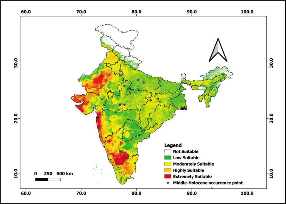
Total seven fossil pollen records of B. monosperma for MH (4,500–7,000 yr BP) were compiled from published papers from Raebareli District, Uttar Pradesh (Saxena et al., 2015), Sehore District, Madhya Pradesh (Quamar & Nautiyal, 2017; Verma & Rao, 2011), Koriya District, Chhattisgarh (Quamar & Bera, 2014, 2017) Hoshangabad, Madhya Pradesh (Chauhan & Quamar, 2012) and Unnao, Uttar Pradesh, (Trivedi et al., 2012).

To assess the performance of SDM for reconstructing the past B. monosperma distributions, we compared the model-based projections with vegetation reconstructions based on fossil pollen data. Reconstructions through fossil pollen data are well consistent with our results based on SDMs. Three fossil pollen records of B. monosperma across the Indian subcontinent for MH (4,500–7,000 yr BP) were compiled from Sehore (Verma & Rao, 2011) and Hoshangabad districts, Madhya Pradesh (Chauhan & Quamar, 2012) and one fossil point from Koriya District, Chhattisgarh (Quamar & Bera, 2014, 2017) is centred in highly suitable habitat. However, two records from Unnao (Trivedi et al., 2012) and Raebareli districts, Uttar Pradesh (Saxena et al., 2015) are concentrated in low suitable habitat. The fossil pollen data supports the distribution of B. monosperma in central India (Madhya Pradesh and Chhattisgarh) and Uttar Pradesh, which are estimated as highly and low suitable habitats respectively in the species distribution maps (Figure 9). B monosperma is common in the forests in the Indian subcontinent but is mainly underrepresented in the pollen data which could be attributed to the low pollen productivity of the plant species as it exhibits a strong tendency of endogamy (Chauhan, 2008; Quamar & Bera, 2014; Quamar & Chauhan, 2011). Hence, the low deposition of its pollen in the sediments along with misidentification of poorly preserved grains is the key factor for the low abundance of B. monosperma pollen in the fossil records.

Impact of Climate Change on B. monosperma

The present study suggests that climate change plays a significant role in controlling the distribution of B. monosperma in the Indian subcontinent. Compared to the current scenario, the habitat suitability of the species is predicted to be reduced during the year 2070 under RCP 2.6, RCP 4.5, RCP 6.0 and RCP 8.5 (Figure 5a–d). Our overall result revealed that by 2070, there would be a decrease in the area of extremely suitable habitat from the current range by 0.97%, 1.58%, 1.51% and 2.19% in future climatic scenarios RCP 2.6, RCP 4.5, RCP 6.0 and RCP 8.5, respectively (Table 5, Figure 7). It was also noticed that the overall reduction in the suitable area is higher under the RCP 8.5 emissions scenario compared to RCP 2.6 emission scenario. Under the RCP 2.6 emission scenario, the average annual temperature is projected to increase by 0.4°C and 1°C by the years 2065 and 2100 century respectively, with the corresponding figures for the RCP 8.5 emissions scenario being 2.0°C and 3.7°C (IPCC, 2013). Across all RCPs, the global mean temperature is projected to rise by 0.3 to 4.8°C by the late twenty-first century (IPCC, 2013). The expected increases in temperatures, as well as seasonal deviation in temperature and precipitation, are the significant, causes of decreasing habitat suitability.

Indian tropical dry deciduous and tropical moist deciduous forests are predominant and account for 34.8% and 7.72% of the total forest area, respectively. Anogeissus latifolia, Anogeissus penduala, Albizia procera, Anthocephalus chinensis, Diospyros melanoxylon are the dominant tree species of dry deciduous forest (Reddy et al., 2015). According to the IPCC, forests around the world would be adversely impacted by climatic and non-climate stresses, which could result in forest die-back, biodiversity loss and impaired ecological benefits (IPCC, 2013). Climate change will exacerbate the risks to our forests and all forests will not be able to acclimatise to the altering climate. Global environmental change is expected to cause ecosystem shifts and the extinction of some species, particularly those that are unable to adapt. Extreme climate events and natural disasters are expected to become more intense, in future climate scenarios (IPCC, 2013). Dry forests, despite their economic and social importance, have received little attention and are one of the most vulnerable and little-understood forest ecosystems (Miles et al., 2006; Portillo-Quintero & Sanchez-Azofeifa, 2010). These forests are in greater danger due to a lack of attention and scientific study (Aide et al., 2013).

Conservation Management

The findings of this study could help establish a conservation approach for B. monosperma in India by recognising the critically vulnerable habitats and probable climatically suitable regions where restoration strategies can be implemented for forest rejuvenation. Our study revealed that the extremely suitable habitat of B. monosperma will withstand in the Nilgiri hills of India. Also, the moderately and low suitable habitats will be sustained in north-eastern and central India regions, respectively. Hence, we recommend active restoration and conservation strategies for this climatically stable area for the protection of B. monosperma in the existing habitat to avoid future extinction. The model also predicted that the suitable habitat would severely decline in future climatic scenarios due to climate change. Therefore, preventive measures should be adopted in those areas that are projected to decline in future scenarios to facilitate the growth of these species. Also, the population of the species must be brought under in-situ conservation programs and needs to be protected strictly and monitored. It is imperative to perform region-wise research and analysis to study the influence of climate change on B. monosperma to establish conservation and management measures. Preservation and re-establishment policies for B. monosperma should be done by taking care of the native people, their expectations and aspirations.

Conclusions

Assessing the future distribution of B. monosperma in response to rapid climatic variations is of major importance for developing strategies for the conservation of B. monosperma. The present study defines the probable changes in B. monosperma distribution in the past (LGM and MH), current and future (2070) climatic scenarios. The habitat suitability of B. monosperma tends to decrease from RCP 2.6 to RCP 4.5 with a further sharp decline from RCP 6.0 to RCP 8.5 during future climatic scenarios (2070). The broader picture of 2070 under different RCPs suggested the potentially suitable habitat will decrease in the southern and western regions and moderately suitable habitat will sustain in the north-eastern region. Model-based species distribution during MH coincides with past proxy-based reconstructions from the region, which supports well-defined refuges of the species. Our study will provide a scientific basis to promote the conservation of B. monosperma and establish reasonable management practices in the projected suitable areas for attaining the optimum quality and production of its resources. Further studies for understanding the distribution processes will be crucial for the rapid extensive migration of the species and its conservation in the coming years.

Supplemental Material

Supplemental material for this article is available online.