Validation of numerically simulated ventricular flow patterns during left ventricular assist device support

Abstract

Intraventricular flow patterns during left ventricular assist device support have been investigated via computational fluid dynamics by several groups. Based on such simulations, specific parameters for thrombus formation risk analysis have been developed. However, computational fluid dynamic simulations of complex flow configurations require proper validation by experiments. To meet this need, a ventricular model with a well-defined inflow section was analyzed by particle image velocimetry and replicated by transient computational fluid dynamic simulations. To cover the laminar, transitional, and turbulent flow regime, four numerical methods including the laminar, standard k-omega, shear-stress transport, and renormalized group k-epsilon were applied and compared to the particle image velocimetry results in 46 different planes in the whole left ventricle. The simulated flow patterns for all methods, except renormalized group k-epsilon, were comparable to the flow patterns measured using particle image velocimetry (absolute error over whole left ventricle: laminar: 10.5, standard k-omega: 11.3, shear–stress transport: 11.3, and renormalized group k-epsilon: 17.8 mm/s). Intraventricular flow fields were simulated using four numerical methods and validated with experimental particle image velocimetry results. In the given setting and for the chosen boundary conditions, the laminar, standard K-omega, and shear–stress transport methods showed acceptable similarity to experimental particle image velocimetry data, with the laminar model showing the best transient behavior.

Introduction

Left ventricular assist devices (LVADs) have become a long-term treatment option for patients with heart failure ¹ and significant improvements in survival rate and quality of life have been observed, ² with a comparable or even superior outcome compared to cardiac transplantation. ³ However, thromboembolic events are a major complication of LVAD therapy with a reported stroke rate of 0.14–0.18 events per patient-year. The LVAD changes the intraventricular flow patterns^1,4–6 and probably results in areas that favor thrombus formation like stagnation areas, recirculation zones, non-physiological shear stresses, and large blood residence times.^7–10 However, clinical imaging methods for cardiac flow field investigations in LVAD patients with adequate spatial and time resolution are still limited. Echocardiography is mainly used to monitor cardiac functionality and is limited to unidirectional velocities. Echo particle image velocimetry (PIV) is not yet available in clinical routine^11–13 and magnetic resonance imaging cannot be used in LVAD patients because of the large metallic pump bodies. ¹⁴ Therefore, investigations of flow fields in supported hearts demand either experimental or computational modeling: on one hand, PIV gives noninvasive access to actual instantaneous velocities in single planes, but requires flawless transparent models and good optical access. On the other hand, computational fluid dynamics (CFD) can provide additional insights into complex three-dimensional (3D) flow fields and immeasurable quantities in any region. However, since there is no analytical solution for the Navier–Stokes equation, CFD uses different numerical schemes to approximate the flow fields. Therefore, the results of the simulations need to be validated against experimental results.

To evaluate the reliability of CFD simulations, the US Food and Drug Administration (FDA) initiated two benchmark studies by comparing standardized simulations to PIV experiments. In intentionally simple geometries, consisting of a nozzle combined with a sudden expansion ¹⁵ and a plain blood pump, ¹⁶ results showed that various numerical methods (laminar (LAM), shear–stress transport k-omega (SST), standard k-omega (SKO), and renormalized group k-epsilon (RNG)) performed differently and in some cases showed large deviations from the experiments. The blood pump benchmark study ¹⁵ concluded that flow fields simulated by CFD methods require careful validation especially in terms of shear–stress distributions, recirculation, hemolysis, and thrombosis evaluation. ¹⁶

The aim of this study was to compare the experimental flow in an LVAD-supported cardiac model with several numerical solvers with accurately defined boundary conditions to determine the best fitting algorithm.

Materials and methods

Left ventricular model

The computed tomography (CT) scan of a patient suffering from dilated cardiomyopathy was used (Figure 1(a)) to create a simplified polyethylene reservoir based on the segmentation of the CT data. ¹⁷ The volume was within the range suggested for chamber quantification studies ¹⁸ and the left ventricle (LV) model was kept intentionally simplified to provide more generalized information.

Figure 1.

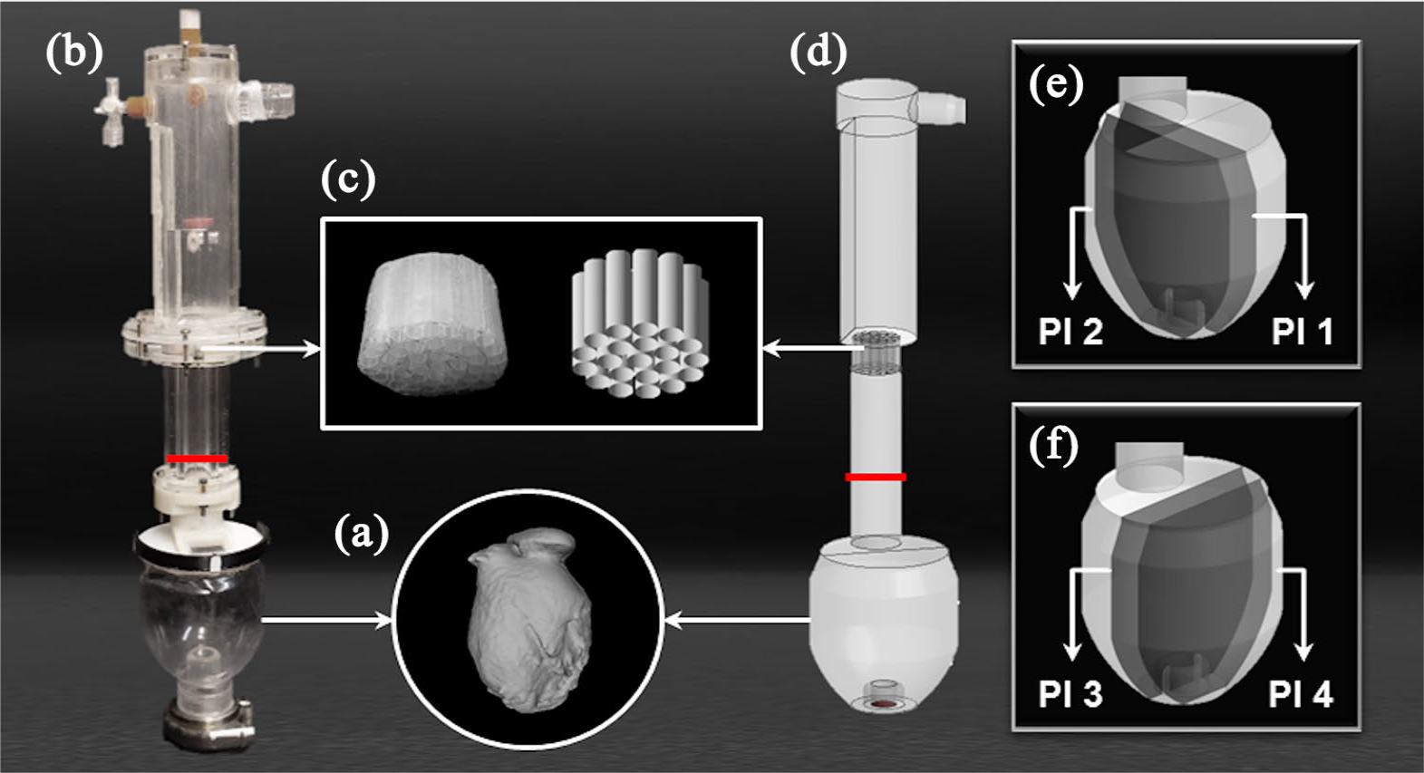
Overview of the experimental and numerical model: (a) CT scan of a dilated ventricle, (b) PIV model, (c) flow straightener, (d) CFD model, (e) the medial (Pl 1) and the side (Pl 2) coronal planes, and (f) the medial (Pl 3) and the side (Pl 4) sagittal planes.

Particle Image Velocimetry

The experimental setup consisted of a mock loop setup with an LVAD (Medtronic HVAD^®, Dublin, Ireland) connected to a transparent LV model (Figure 1(b)). The model geometry was immersed in a fluid-filled tank and the mock loop and the surrounding tank were filled with a blood analog mixture of glycerol and water (40% glycerol). At the inflow of the cardiac model, a well-defined inflow section containing a flapper plate and a flow straightener (Figure 1(c)) was used to create consistent inflow conditions, as skewed or rotational inflow could have strong effects on the flow fields inside the ventricle. The pump speed was set to 2400 r/min, and the flow rate of the LVAD was set to 3.5 L/min.

The mock loop was seeded with fluorescent polystyrene microspheres (1.06 g/mL with mean particle size of 10.5 µm). A pulsed Nd:YAG-Laser system (NANO L 20-100 PIV double oscillator laser system, Litron Lasers, Rugby, UK) was used to illuminate the particles inside the LV model and image pairs were captured using a SpeedSense9020 CMOS camera (Vision Research, NJ, USA) with a resolution of 1152 × 896 pixels at a rate of 50 Hz. In order to allow validation over the whole ventricular model, 46 planes (23 in coronal and 23 in sagittal directions) were recorded at 3-mm intervals starting from the midplane, using a mirror to create the orthogonal imaging planes. About 2100 image pairs were recorded per plane, which resulted in 42 s of recording for every plane. The time between pulses was selected individually based on the one-quarter displacement rule, ¹⁹ depending on the local velocities of the plane, with values ranging from 2 000 µs for higher velocity flow fields to 10 000 µs for images captured close to the edges of the model. PIV data analysis was performed in DynamicStudio™ (v3.41, Dantec Dynamics, Skovlunde, Denmark) using the Adaptive Correlation Algorithm with an interrogation area of 32 × 32 pixels with 50% overlap. The calculated vector maps were exported to MATLAB (The MathWorks, Inc., Natick, MS, USA) for data evaluation.

Hemodynamic parameters were recorded at 100 Hz using a controller board (DS1103 PPC Controller Board, dSPACE GmbH, Paderborn, Germany). Pressures were captured using disposable pressure transducers (TruWave, Edwards Lifesciences LLC, Irvine, CA, USA) and transducer amplifiers (TAM-A, Hugo Sachs Elektronik—Harvard Apparatus GmbH, March-Hugstetten, Germany) at the inflow cannula (IC) and at the outflow of the LVAD. The flow rate was measured at the outflow of the LVAD (Transonic H9XL flow probes, HT110R flowmeter, Transonic Systems Inc., Ithaca, NY, USA).

Computational Fluid Dynamics

Geometry

The model geometry including the inflow section used in the experiments was used as a basis for the CFD geometry design and created in ANSYS DesignModeler (ANSYS 16.1, Inc., Cecil Township, Pennsylvania, USA; Figure 1(d)).

Meshing

A fully hexahedral mesh with 5,000,000 elements was created for the whole geometry to improve convergence and solution time in ANSYS meshing (ANSYS 16.1, Inc., Cecil Township, Pennsylvania, USA). The size of the mesh elements at the LV volume was set to 0.45 mm and at the apical area the size was reduced to 0.35 mm, to capture fluid behavior close to the cannula. The mesh quality was within ranges recommended by ANSYS Meshing Users Guide with no element possessing skewness above 0.83 and orthogonal quality below 0.23. ²⁰

For the calculated mesh, a y-plus value was 1.2 that allowed the use of the enhanced wall treatment function for the RNG model. ²¹

To guarantee mesh independency, a finer mesh with 7 million elements was used for the simulations. The results of the mesh independency study can be found in the supplemental material.

Boundary conditions

Blood was modeled as a Newtonian fluid with a constant density of 1050 kg/m³ and a dynamic viscosity of 0.0035 Pa s. A mass flow inlet with a constant flow rate of 3.5 L/min in a perpendicular direction to the inlet was set as a boundary condition at the inlet. The pump cannula outlet was set as an outflow boundary condition. The no-slip boundary condition was chosen for all walls.

Solver settings

A commercial unsteady incompressible finite-volume solver (FLUENT, ANSYS 16.1, Inc., Cecil Township, Pennsylvania, USA) was used to solve the mass and momentum conservation equations with four different numerical methods consisting of LAM, SKO, SST, and RNG. A pressure-based solver with second-order upwind scheme spatial discretization was selected for the pressure, momentum, and continuity equations. The transient simulation was performed for 7 s with a step size of 0.001 s and 10 s of initialization, to guarantee a fully developed flow field. The convergence was achieved in each time step when the residuals were below 10^–3 for continuity, x-velocity, y-velocity, z-velocity, and turbulence parameters (for SKO, SST, and RNG). All simulations were performed on the Vienna Scientific Cluster.

Regions of interest

The comparison analysis was performed for both flow field data and scalar quantities in the 46 planes recorded in PIV: 23 in coronal and 23 in sagittal cross-sections. The planes were defined with 3 mm offset from each other, starting from the midplanes. For a direct comparison of the numerical simulation to the experimental recording, the results were interpolated on the PIV grid for all planes.

Four planes were selected as representative planes for both high- and low-velocity regions. Therefore, two coronal planes (Figure 1(e)) were chosen in the range of mitral annulus diameter to compare the flow characteristics around the main flow jet: medial coronal plane (Pl 1) that passes through the center of the mitral annulus and IC, and side coronal plane (Pl 2) 12 mm dorsal of the IC center. Also, the positions of two sagittal planes (Figure 1(f)) were defined to visualize the flow pattern far from the main flow as well as recirculation zones around the IC: medial sagittal plane (Pl 3) that passes through the center of the IC and side sagittal plane (Pl 4) 12 mm ventral of the IC center.

Quantitative analysis

Velocity magnitude

The simulated flow fields were compared to experimental results using the mean velocity magnitude.

Stagnation regions

Stagnation regions are considered as potential regions for thrombus formation; however, there is no universally defined range of velocity magnitude values to characterize these areas. To identify areas of stagnation, the area with an absolute velocity magnitude value below 10 mm/s was calculated.

Validation metrics

The mean of the local absolute error was used to compare the different CFD methods with the experimental measurements (equation (1))

$$E=\frac{1}{N}{\displaystyle \sum }_{i=1}^N\left|u_{e,i}-u_{c,i}\right|$$

(1)

where $N$ is the number of the PIV vectors, $u_{e,i}$ and $u_{c,i}$ show the experimental and CFD average velocity, respectively, over time at grid position i, and $E$ is a non-negative value that describes the similarity of two datasets. For $E=0$ the vector field of the CFD simulations matches the field of the experimental results.

Standard deviation of the velocity magnitude

The transient flow characteristics were compared by calculating the standard deviation (SD) of the velocity field.

Results

Inflow velocity profile

The well-defined inflow section created the same inflow velocity profile at the mitral position for both the numerical simulation and the experimental setup. The final velocity profile flowing to the LV through the mitral annulus (the red line in Figure 1(b) and (d)) is shown in Figure 2 with the variation over time (SD) shown in the error bar plots and compared to the CFD results.

Figure 2.

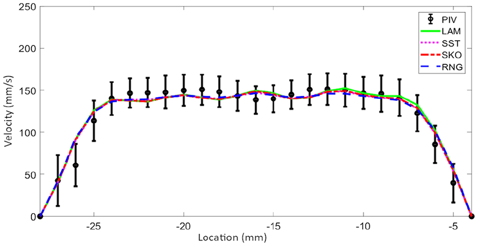
Mean velocity magnitude profile along the lines 30 mm above the inlet of left ventricular model for PIV and all CFD methods: LAM, SKO, SST, and RNG.

Velocity patterns

The flow fields showed a well-developed jet coming from the inflow section and being redirected toward the IC. A large part of the flow was also recirculated along the ventricular walls in the coronal midplane (Figure 3(a), Pl 1).

Figure 3.

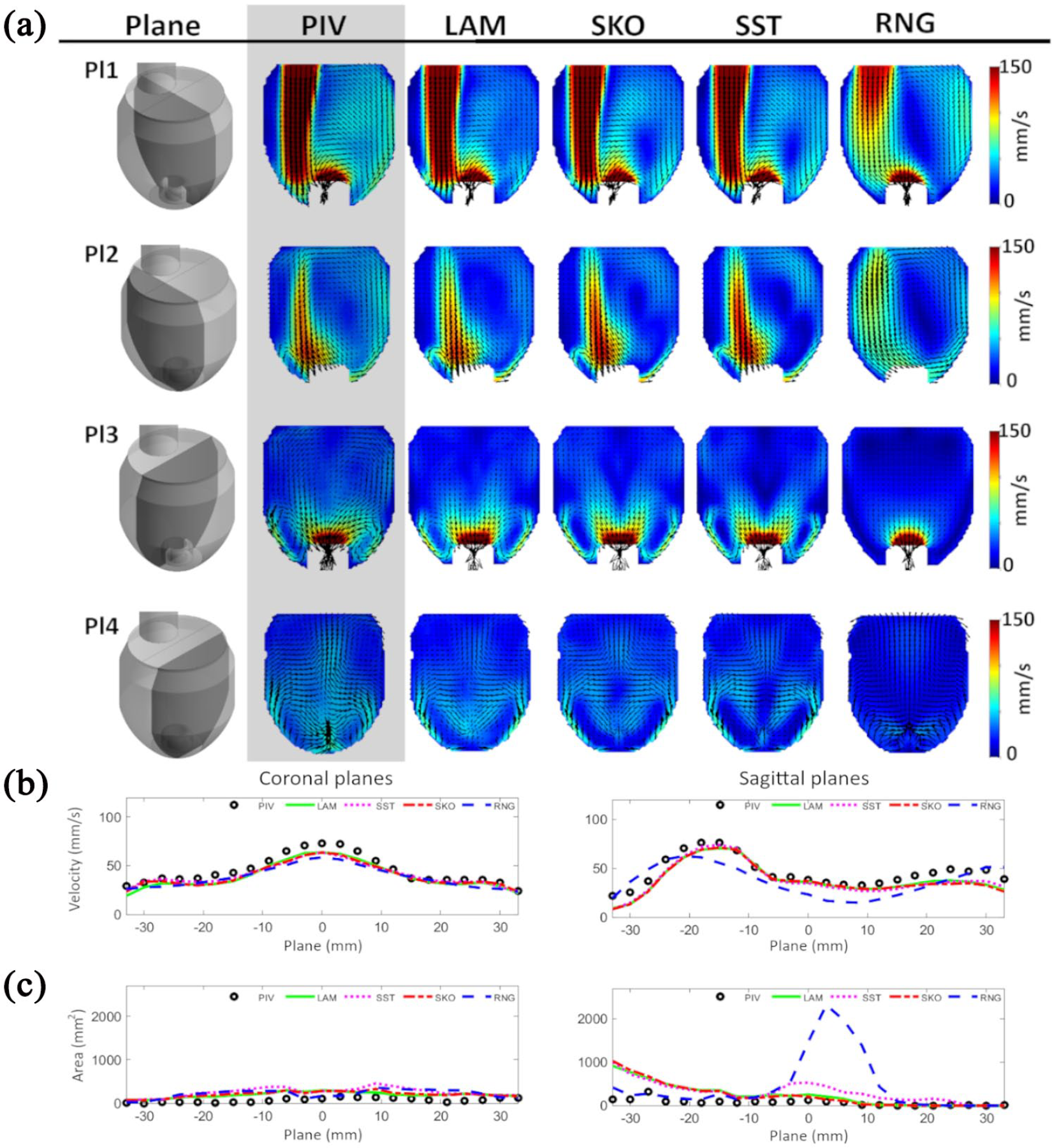
(a) Contour of mean velocity magnitude with velocity vector fields (top to bottom): the medial coronal plane (Pl 1), the side coronal plane (Pl 2), the medial sagittal plane (Pl 3), and the side sagittal plane (Pl 4); (b) mean velocity magnitude; and (c) stagnation regions (V < 10 mm/s) over all 46 planes in coronal and sagittal directions.

Comparable flow patterns were seen with the LAM, SKO, and SST methods for most of the planes; however, the RNG method already failed to predict the major inflow jet pattern. At the medial coronal plane (Figure 3(a), Pl 1), the RNG method could not predict the main flow stream coming from the mitral annulus, where the blood enters the ventricular cavity. Also at the side coronal and the medial sagittal cross-sections (Figure 3(a), Pl 2 and Pl 3), the results for the RNG methods deviated from the experiment and the occurrence of apical vortices was not seen, while the other methods clearly showed these vortices around the IC. In the sagittal directions, very distinct symmetric behavior was observed in the simulations, while the flow fields of the experiments were slightly skewed to one side (Figure 3(a), Pl 3 and Pl 4).

The mean velocity magnitude and the stagnation areas for all planes are represented in Figure 3(b) and (c), respectively. All of the numerical methods, except RNG, could recreate the mean velocity pattern of the PIV results. Large stagnation areas were predicted with the RNG method around the center of the LV chamber which can be seen in Figure 3(c), bottom row in the planes located from −5 to 15 mm in the sagittal direction. This behavior was also observed in the velocity contour plots for the sagittal planes (Figure 3(a), Pl 3 and Pl 4).

Validation metrics

A high absolute error of the CFD results compared to the PIV experiments around the main flow jet was seen for LAM, SST, and SKO in both coronal planes (Figure 4(a), Pl 1 and Pl 2). Lower errors were seen in sagittal planes (Figure 4(a), Pl 3 and Pl 4); the SST method, however, showed a comparable high error at the recirculation zones around the IC (Figure 4(a), Pl 4).

Figure 4.

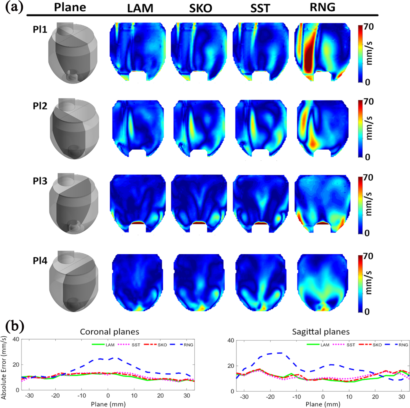
(a) Contour of absolute error of the velocity magnitude (top to bottom): the medial coronal plane (Pl 1), the side coronal plane (Pl 2), the medial sagittal plane (Pl 3), and the side sagittal plane (Pl 4) and (b) absolute error of the mean velocity magnitude over all 46 planes in coronal and sagittal directions.

The mean absolute error was similar for the LAM, SKO, and SST methods, while the RNG method showed higher errors in planes crossing the mitral inflow where blood enters the model (Figure 4(b)). Absolute mean error values for the velocities over the whole LV volume were similar for all except the RNG method (LAM: 10.5, SKO: 11.3, SST: 11.3, and RNG: 17.8 mm/s). The lowest absolute error was seen in 23 of 46 planes for LAM, in 3 planes for SKO, in 14 planes for SST, and in 6 planes for RNG.

SD of velocity magnitude

Transient flow behavior was observed inside of the ventricle mostly around the main flow jet because of the Kelvin–Helmholtz instability. In both coronal planes (Figure 5(a), Pl 1 and Pl 2), the high-flow variation over time occurred because of the vortical structure around the main flow jet. This behavior was more pronounced in the experimental results and captured to a limited extent only by the LAM method. The rest of the numerical models showed a much smaller variation. On the sagittal side (Figure 5(a), Pl 3 and Pl 4) overall less variation was found, which was not captured to the true extent by any of the methods. However, the LAM method partially showed some limited variation. The SST and RNG methods completely underestimated the variation.

Figure 5.

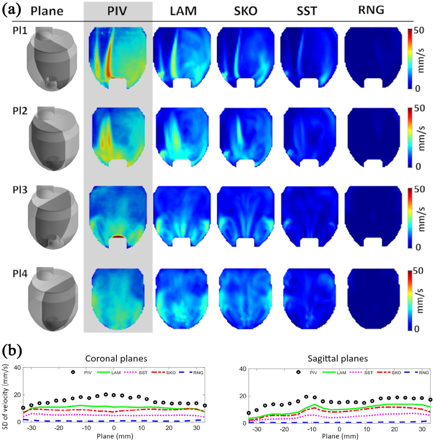
(a) Contour of standard deviation of the velocity field (top to bottom): the medial coronal plane (Pl 1), the side coronal plane (Pl 2), the medial sagittal plane (Pl 3), and the side sagittal plane (Pl 4) and (b) standard deviation (SD) of the velocity magnitude over all 46 planes in coronal and sagittal directions.

Overall the PIV measurements showed the highest variation over time around the main flow stream, a feature that was not simulated successfully by any method. Figure 5(b) shows the SD of the velocity field for the whole LV.

Between all simulations the LAM method showed the highest variation of velocities, being closest to the values measured in PIV over the whole LV (PIV: 16.2, LAM: 10.6, SKO: 8.8, SST: 5.0, and RNG: 0.7 mm/s).

Discussion

Non-physiological flow patterns in LVAD patients and abnormal stagnation areas within the ventricle were previously identified in experimental flow models,^22,23 in CFD models.^24–26 However, since there is no clinical method applicable for LVAD patients to visualize the ventricular flow fields, in-vitro experiments and numerical simulations are still important tools for gaining insights into the flow patterns with specific limitations.

Especially CFD can be a valuable tool to investigate highly 3D intraventricular flow fields during LVAD support. However, since CFD is the approximation of the flow fields and there are different numerical methods, the accuracy of the CFD simulations needs to be experimentally validated using PIV experiments. ²⁷ Based on different turbulence regions and specific Reynolds numbers, careful consideration of turbulence models is mandatory (e.g. direct numerical simulation, LAM, SKO, SST, RNG, and realizable k-epsilon). ²⁸ However, at the mitral valve, ²⁸ the Re number can vary from 700 to 6500 during diastole alone, and the selection of the most adequate turbulence model remains unclear. The simulation of the intraventricular flow field has been performed with the LAM method.^24,26 However, the FDA nozzle study identified issues for Re numbers larger than 500 in predicting main flow features downstream of an expansion. ¹⁵ Due to the highly dynamic flow already at the mitral inflow into the LV, it is impossible to identify one method that perfectly fits. The experimental flow behavior inside the ventricle is neither fully laminar nor fully turbulent rather it is most accurately described as being in the transitional flow regime.

Therefore, we performed a comparative study between CFD simulations applying different numerical models and PIV experiments for the appropriate selection of CFD methods. The accuracy of four numerical methods that cover the laminar, transitional, and turbulent flow regime in simulating the ventricular flow fields was assessed in this study. The results of the simulations were then compared to experimental data. Different parameters were used to determine the accuracy of each method including velocity magnitude, its SD, the absolute error of the velocity magnitude, and area of low-velocity regions.

Overall, the flow patterns simulated by LAM, SKO, and SST methods showed good agreement with experimental results, since the flow behavior can be best attributed to the laminar and transitional flow regimes. In this comparison, the RNG method failed to accurately track the main flow stream downstream of the mitral position and was ascertained as an inappropriate method. This behavior probably occurred because the flow is not in the fully turbulent regime since the k-epsilon is intended for this flow regime. Through the absolute error of the velocity magnitude even small differences between the simulated and experimental flow fields were visualized (Figure 4(a)), and large differences in low-velocity flow areas were highlighted. All numerical methods showed signs of over-prediction of low-velocity regions; therefore, there was no definitive best CFD method to accurately identify locations of the stagnation and consequently probable thrombus formation sites.

Velocity variations over time were underpredicted by all numerical methods, but the LAM method showed the most similar behavior compared to PIV. The other methods, most notably SST and RNG, highly underestimated these variations. This is probably because the simulations are based on temporal and spatial averaging, which decreases the likelihood of including small-scale eddies in the final flow field.

Although the main characteristics of the flow fields were simulated, some limitations still remain. A number of assumptions had to be made that allowed direct comparison between experimental results and four different numerical methods:

• The mitral valve leaflets were not included in the model since the complex structure of these valves is yet to be implemented in CFD simulations.

• The fluid was considered Newtonian.

• This study was done under stationary conditions; a further study may be required for higher flow rates and pulsatile conditions.

Therefore, the analysis has to be considered as a comparison between different numerical methods against experimental work in clearly defined conditions that cannot cover every imaginable variation in conditions and individual LV geometries.

Conclusion

Experimental validation of CFD methods is an often overlooked aspect not only for intraventricular flow patterns. The characteristics of the intraventricular flow fields from PIV results, such as jets and vortical structures, were simulated using four different numerical methods. For the chosen boundary conditions, intraventricular flow patterns using LAM, SKO, and SST were comparable to the experimental results. By comparing the transient behavior of the velocity field, the LAM method predicted more accurate results than other CFD methods.

However, for detailed analysis of flow patterns and its connection to thrombosis risk evaluation, further studies are required to link the findings with clinical results or blood tests. This aspect further remains a critical challenge for patient-specific geometries with different support conditions.

Supplemental Material

Supplemental_Material_Mesh_Study_Revision_V1.0 – Supplemental material for Validation of numerically simulated ventricular flow patterns during left ventricular assist device support

Supplemental material, Supplemental_Material_Mesh_Study_Revision_V1.0 for Validation of numerically simulated ventricular flow patterns during left ventricular assist device support by Mojgan Ghodrati, Thananya Khienwad, Alexander Maurer, Francesco Moscato, Francesco Zonta, Heinrich Schima and Philipp Aigner in The International Journal of Artificial Organs