Food for Survival

Abstract

Background:

Burundi is one of the world’s poorest countries, coming last in the Global Food Index (2013). Yet, a large majority of its population depends on agriculture. Most smallholder families do not produce enough to support their own families.

Objective:

To estimate the optimal crop mix and resources needed to provide the family with food containing sufficient energy, fat, and protein.

Methods:

This study uses mathematical programming to obtain the optimal crop mix that could maximize output given the constraints on production factor endowments and the need to feed the household. The model is calibrated with household-level data collected in 2010 in Ngozi Province in northern Burundi. Four models are developed, each representing a different farm type. The typology is based on 2007 data. Model predictions are compared with data collected during a revisit of the area in 2012.

Results:

By producing a smaller number of crops and concentrating on those in which they have a comparative advantage, and trading produce and input with other farms, large and medium-sized farms can improve their productivity and hire extra workers to supplement family labor. Predictions of crops to be planted coincided to a high degree with those that farmers planted 2 years after our survey on newly acquired plots.

Conclusions:

Despite land scarcity, it is still possible for households that own land to find optimal crop combinations that can meet their minimal food security requirements while generating a certain level of income. Nearly landless households would benefit from the increased off-farm employment opportunities. With only 0.05 ha of land per capita, the annotation Nearly Landless is used to highlight the limited access to land observed in this farm category.

Keywords

Burundi food insecurity production model resource allocation small farms specialization

Introduction

The way agriculture can contribute to food security is well established, whereas recently new attention has been given to the role of agriculture in nutrition.^1,2 A key role for agriculture is to provide nutritious food to the households that produce it.¹ Agricultural growth is expected to contribute to food and nutrition security, both directly (e.g., by autoconsumption) and indirectly (e.g., by income generation).¹ Such agricultural growth is to be expected from increased farm productivity through adoption of technology and improved access to inputs, inclusion in food value chains, and favorable policy environments.^1
-3 Yet, many poor African rural households still face food insecurity. Paradoxically, poor African rural households, which often depend heavily on subsistence farming, seem unable to cover their own minimum food needs.^4
-6 The dominant production systems in the poorest areas are still characterized by low input use, mixed cropping, and keeping a small number of livestock, with a high degree of reliance on their own production to provide their food. Besides problems of land scarcity and soil degradation, smallholder farmers operate in an environment of incomplete and poorly functioning markets for labor, land, credit, commodities, risk, and information⁷, while support policies are limited.⁸ This partly explains the persistent low crop productivity, food insecurity, hunger, and malnutrition among poor African agriculture-based communities.⁹

The obvious question is what would be needed to realize what Haddad calls “the elusive potential of agriculture for nutrition”¹ and food security. Haddad calls for the development of diagnostic tools that enable identification of leverage points on issues such as crop choices, investment areas, agricultural extension, and access to inputs and markets.¹ Turner et al.² describe the gaps in methodologies and metrics in research on agriculture and nutrition, and express concerns over the limited research on agricultural policy and governance issues. In this paper we try to address—or at least touch upon—these issues. We propose a mathematical model to predict which cropping patterns may be most appropriate to provide food security to different groups of farmers in the poor rural areas of northern Burundi. Perhaps we do not fully answer Haddad’s question, because we are more concerned with the provision of minimal amounts of food to feed a household and secure its macronutritional composition than with the availability of micronutrients. Yet, given the dire food-insecure situation of poor Burundian households, we think such an initial approach is valuable.

While food demand in Burundi continuously increases as a result of population growth, declining land availability and increasing rural poverty hamper further growth in production and agricultural development. Over the years, and reinforced by the political crises, food insecurity and poverty have worsened. Burundi has a sad record of coming last in the International Food Policy Research Institute Global Hunger Index of 2013. An estimated 90% of Burundians depend on agriculture for their livelihoods, but farms are small and mainly use mixed cropping systems supplemented with a small number of livestock and secondary commercial production of bananas, coffee, and tea.

This paper aims to analyze the optimal crop mix and resource use that maximize crop output to cover household food needs in terms of energy and macronutrients. A mathematical program is used to calculate the optimal crop mix that could maximize output given the constraints in production factor endowments and the need to feed the household. The models also account for possible trading of resources between farmers. We attempt to show that changes in crop choices may contribute to improved food self-sufficiency, but also that relative resource constraints strongly determine the optimal crop combination. A comparison of the results between farms with different endowment levels allows us to determine how such resource constraints influence optimal crop mixes.

We use detailed farm-level data that were collected in the north of Burundi in 2007, 2010, and 2012. A typology of four farm types is based on the 2007 data. A subsample was revisited in 2010 and 2012. The mathematical model is calibrated with the 2010 data. The predictions made by the model are compared with crop production trends recorded in the 2012 data. Since no specific policy toward crop specialization has been implemented since 2007, the trends in crop production measured between the two records are a result of population pressure, changes in land tenure, and market forces (e.g., recent liberalization of the coffee market).

Mathematical models have been used for years to analyze optimization processes at a microeconomic level.¹⁰ The models are embedded in the land rent theory of Von Thünen and Ricardo, and depart from the premise that all parcels of land, given their attributes and location, are used in the way that earns the highest rent.¹¹ The key argument of specialization goes back to Ricardo’s claims for labor division, comparative advantages, and trade. Yet, poor infrastructure, high transport costs, and the bulky nature and perishability of many of Africa’s staple food crops put limits on crop specialization, intraregional trade, and large-scale exchanges.⁸ Given the poor resource base of farmers we deal with in this paper, we believe the greatest scope lies in domestic markets, and efforts should be geared toward improving intrarural systems of distribution.

We believe this paper is original for at least three reasons. First, the mathematical program is used as a diagnostic tool to predict what crop choices could secure production that covers minimal nutrition requirements in terms of caloric content and macronutrients, while at the same time fitting the realities of subsistence production systems. It also allows for trade between different types of farm. Second, the paper distinguishes farm types identified by cluster analysis. Although all farmers in the study area are considered smallholders, relatively small differences in endowment levels have an important effect on crop choice, production, and productivity. Hence, development paths need to be identified by farm type.¹² Finally, because the research area was recently revisited, we were able to check whether the outcome of the model correctly predicts the changes in crop production.

Research Background

Agriculture Sector in Burundi

Burundi is a landlocked country in the Great Lakes region of Eastern Africa. It is a resource-poor country with an underdeveloped manufacturing and service sector. With an urbanization rate close to 10%, almost 90% of the population lives in rural areas with agriculture as their main activity.¹³ Rural livelihoods are closely tied to agriculture as a source of food and income.¹⁴ The sector employs 90% of the workforce through small-scale, subsistence-oriented family farming units and accounts for 95% of the food supply. Agriculture represents more than 50% of GDP, and over 80% of export earnings come from the export of coffee.¹⁵

In the past, adequate rainfall patterns and good soils made Burundi self-sufficient in food production.¹⁶ However, high population density has produced a considerable increase in pressure on arable land, which has gradually led to expansion of cultivated areas over marginal lands, but also to a reduction in the average surface area per household and widespread underemployment in the countryside. This has forced farmers toward a progressive and continued intensification of cropping systems, with two main components: the multiplication of crop cycles and the spread of mixed or multiple cropping, with progressive disappearance of interspersed fallow periods; and the development of banana cultivation¹⁷ because of its prominent position in the farming system and its multipurpose character.¹⁸ An estimated 85% of total cultivated land is used for food crop production, which, together with livestock, is the main source of food and income for most households.¹⁹

Nearly all households grow a diverse mixture of food crops, sometimes associated with cash crops and some animals.¹⁵ Animal production (milk, eggs, meat) is usually low or erratic (e.g., goats are slaughtered for particular celebrations), suggesting that livestock is mainly kept for manure, draught power, savings, security, and social status.^17,19 The leading agricultural products can be classified into cash crops, food crops, and horticultural products. The most important cash crop is coffee, followed by tea and cotton.¹³

Household Food Security Situation

Low agricultural returns have seriously affected farmers’ ability and motivation to invest in their farms. The capacity of land and labor to supply food in sufficient amounts has been compromised, imports of food are increasing steadily, and the country is depending heavily on aid from bilateral and multilateral donors. Subsistence crop production has grown more slowly than the population, while export crop production has fallen.^13,20 Per capita agricultural productivity has been declining for years, with obvious implications for food and nutrition security. Studies point to high poverty levels, with 70% of the population living below the national poverty line and 63% gripped in a severe food-insecurity situation.^15,21 Options for rural employment (which should create job opportunities capable of absorbing the excess rural labor) are often limited to informal labor exchange between farms during critical periods. It is against this background that we study the potential for optimizing farm production systems.

Materials, Methods, and Study Techniques

Study Area

This study was conducted in Ngozi, a province located in the north of Burundi. The rationale for selecting this area for the study was suggested by both demographic and agricultural features of the region. Ngozi ranks among the most overpopulated provinces of Burundi, with an average population density of 462 inhabitants per square kilometer. The province ranks fourth of 17 provinces of Burundi in agricultural production.²²

Sampling Procedure and Data Collection

Household data on farm activities in Ngozi were gathered in three survey rounds in 2007, 2010, and 2012. In 2007, 640 households were interviewed in Ngozi and the neighboring province of Muyinga. In each village or commune (9 in Ngozi and 7 in Muyinga) of each province, 10 collines or hills (institutional demarcation) were sampled, from which four households were randomly selected. This sampling procedure tried to capture the variability of the farms across the provinces. However, because of some irregularities in the data, 6% of the households (39 households) were removed from the sample, and the remaining households were clustered into four farm types.

Across these types, a sample of 60 farms was purposely chosen to be interviewed in 2010. The 2010 survey collected more detailed information on production and input use than the 2007 survey. In 2012, 340 households in Ngozi that were interviewed in 2007 were revisited. This resulted in a panel dataset that was used to validate the predictions of the model.

The interviews in Kirundi were done by a team of researchers from the University of Burundi. The questionnaire inquired about household, farm, and farming system characteristics. The farm input and output data covered one production year, which consisted of three cropping seasons designated as 2009C, 2010A, and 2010B. The questionnaire also included questions on expenditure on different farm inputs and various additional household expenses.

Agroecological Environment of Ngozi

The province of Ngozi lies on the central plateau of Burundi. The dominant landscape is a succession of hills separated by wide valleys that characterize the Buyenzi ecological region, with a moderately high altitude of 1,700 m.²² The central plateau has cool weather, with an average temperature of 20°C. The region has a humid tropical climate tempered by altitude, which is said to be one of the reasons for the high population density in the region.

The region has a bimodal rainfall pattern, which allows three cropping seasons per year. The first rainy season (A), known as Agatasi, occurs between October and January. The second season (B) is called Impeshi and lasts for 5 months from February to June. A short dry season (with less frequent and intense precipitation) is observed between these two rainy seasons from mid-January to mid-February, which allows farmers to handle agricultural produce from the first cropping season. The third cropping season (C), called Ici, occurs between July and September. In this dry period, farmers mainly grow vegetables, beans, maize, potatoes, and off-season crops such as rice in wetlands and in river valleys.

In general, the rainy season lasts about 8 months and the dry season 4 months. However, the rainy season has been shorter in recent years. The annual rainfall varies between 1,200 and 1,500 mm.

Farm Typology and Data

The first step of the study consisted of running a cluster analysis on the original (2007) dataset. The aim of the analysis was to construct a farm typology that could serve as a sampling frame for the 2010 data. The typology was based on variables that are indicative of agricultural trajectories and the strategies employed by farmers in sustaining household survival, which are, at the same time, linked to farm characteristics (available land per capita; availability of labor; proportion of cash crops, food crops, and bananas in total output; livestock; and share of nonfarm earnings) (see Appendix Table 1, available online, for more information on the results of the clustering exercise). Next, a subsample of farm households was selected to be interviewed in 2010 to obtain a smaller dataset of 60 farm households on which further analyses were performed. In a third step, the validity of the model was checked with the outcomes of a panel dataset (2007–12) with 340 observations that provides a detailed overview of changes in production of the main crops.

Typically, production systems and livelihood strategies of rural households in less-favored areas are characterized by a wide diversity of resource endowments, activity choices, and the prevailing conditions for engagement in market exchanges.²³ It is unusual to find two identical agricultural production units. Therefore, the ideal development strategy would be to distinguish between all individuals and to find a unique solution for each of them, which is obviously unaffordable.^24,25 Furthermore, one-fits-all policies will not provide an adequate solution in a situation of great diversity.²³ To deal with this marked diversity in possible development paths followed by different farms, it is worthwhile to categorize the sector into subsets showing a maximum amount of heterogeneity between farm types, while obtaining maximum homogeneity within particular categories.²⁴ A good farm typology accounts for the success of research operations and planning of rural development²⁵ by increasing the general applicability of recommended solutions generated by mathematical programming models.²⁴ However, for such models to be effective as a diagnostic tool, they have to be constructed for truly typical or representative situations.²⁴

Havard et al.²⁶ suggest two variants of agricultural development typology: a typology that is structure-based, using available production factors on the farms to distinguish the groups; and a functional typology that considers the process of production and the farmer’s decision-making. We used proxies for both in our cluster analysis. The variables considered in the study for classification are resource endowments (land, labor, livestock), agricultural practices (proportion of cash crops, food crops, and bananas), and household income diversification (nonagricultural income). Bananas are considered a semicash crop because they are important for both household food supply and income the year round.

Modeling Framework

Mathematical programming has become an important and widely used tool for analysis in agriculture and economics. The basic reason for using programming models in agricultural economic analysis is straightforward: the fundamental economic problem is how to make the best use of limited resources.²⁷ These models have been successfully used to improve the planning of agricultural systems.²⁸

The models in this study maximize the annual farm output (three cropping seasons: A, B, and C) (expressed in monetary terms), taking into account limited production factors at the farmer’s disposal (land, labor, and capital or the amount of money annually invested in agricultural production) and the availability of sufficient primary macronutrients for the household throughout the year. Data from 60 farmers across the four farm types were used as input for mathematical programming.

Farm output is measured by the sum of the market value of all crops produced, regardless of whether these are sold or consumed by the household. Farm production for each food crop is multiplied by the average market price of the respective crop.

Although we are aware of the diversity in livelihood of farm households in the study area, for simplicity, activities in the model are limited to crop production. Fifteen crops are identified as major crops capable of providing more than 80% of the household food and income supply; banana (Musa spp.), sweet potato (Ipomoea batatas), cassava/manioc (Manihot spp.), avocado (Persea americana), beans (Phaseolus vulgaris), potato (Solanum tuberosum), rice (Oryza sativa), maize (Zea mays), sorghum (Sorghum bicolor), colocase/taro (Colocasia esculenta), groundnut (Arachis hypogaea), peas (Pisum sativum), soybean (Glycine max), tobacco (Nicotiana tabacum), and coffee (Coffea spp.). However avocado was dropped from the list to eliminate bias, as the crop is perennial and does not require regular maintenance. The model is summarized below:

M a x Z_{l} = \sum_{j k} P_{j} x_{j k l}

Subjected to:

\sum_{j} I_{i j k} x_{j k l} \leq Q_{i k l}

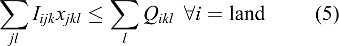
(for all i = 1,…, n; all k = 1, 2, 3; and l = 1, 2, 3, 4)

\sum_{j k} N_{j h} x_{j k l} \geq F_{h l}

\sum_{j} N_{j h} x_{j k l} \geq S_{h k l}

\sum_{j l} I_{i j k} x_{j k l} \leq \sum_{l} Q_{i k l} \forall i = l a n d

x_{j} \geq 0 f o r a l l j = 1, \dots, m)

where

x_{j}

s the level of farm activity j, m the number of activities, k seasons, n the number of constraints, h the types of macronutrients (caloric content [kcal), proteins, and fatty acids), l the number of farm categories, Q the quantity of inputs available, and I the quantity of inputs needed per farm activity per season (Table 1).

Table 1.

Parameters of the Model.

Code	Meaning	Unit
P _j	Price of 1 kg of crop j	US$
x _jkl	Quantity of crop j produced in season k in farm type l	kg
I _ijk	Quantity of input i necessary to produce 1 kg of crop j in season k	US$, hours, ha
Q _ikl	Quantity of input i available in season k in farm type l	US$, hours, ha
N _jh	Nutrient content^a h of 1 kg of crop j	g, kcal
F_hl	Minimum food nutrient h annually required for household type l	g, kcal
S _hkl	Minimum food nutrient h required in season k for household type l	g, kcal

^aCalculation of nutrient content is based on Food and Agriculture Organization table Agriculture, food and nutrition for Africa (http://www.fao.org/docrep/W0078E/w0078e11.htm#P9840_707166).

The model was initially applied to three scenarios, of which two yielded feasible results. Scenario I (market oriented) assumes that agricultural inputs (land, labor, and capital) are the only limiting factors and that they therefore shape the farmer’s decision-making (equation 2). Under this scenario, it is assumed that farmers maximize the value of their output subject to their resource constraints.

Scenario II (subsistence oriented) includes a constraint that production needs to meet the minimum requirements of the households in terms of macronutrients (equation 3). The food nutrient contents (calories, proteins, and fatty acids) of all crops are multiplied by their respective quantities produced and compared with the household food intake needs set as a constraint, because the main goal of the farms is to satisfy family consumption in subsistence agriculture.

Scenario III tried to capture seasonality (equation 4). It tests the seasonal interdependency in providing sufficient production necessary to sustain household food availability. Yet, as will be explained later, the models were unfeasible.

For each scenario, an additional run is performed to assess the impact (on the farm output) of exchanges in production factors between farms, mainly land (equation 5).

The model is applied to representative farms of the four different farm types identified. Four representative farms were purposely selected from each farm type cluster based on the quantity and quality of available information; mainly farms closer to the average in the variables of interest of the farm types were chosen.

This model obviously has limitations. First, the variables considered in the farm typology are mainly resource endowments, agricultural practices, and household income diversification. Other typologies may be developed. Second, we preferred to work with real farm data and not with an average farm per farm type (although the farm with data closest to the average for each type was selected). We believe the production–input balances are more accurate with such an approach. Models with average data may give different results. Third, the same productivity levels are considered per crop. Because of the mixed cropping systems that are applied over the different seasons, it is difficult to estimate the productivity levels for each individual farm. The productivity levels are determined based on own calculations and reports.

Results

Descriptive Analysis

Types of farm households and their characteristics

From the results and findings, four farm clusters are distinguished (see Appendix Table 1A for cluster analysis in 2007 data and Table 2 for 2010 data). These are large, medium, small, and nearly landless farms. With only 0.05 ha of land available for individual household member, the annotation Nearly Landless is used to highlight the limited access to land observed in this farm category. Large and medium farms (32% of the sample) have more land per capita with low availability of labor per unit of land. Small and nearly landless households (68% of the sample) have an excess of labor and a high rate of livelihood diversification into low-paid agricultural work. Previous analyses of the 2007 dataset highlighted that the poorest groups had a higher likelihood of participating in off-farm activities, suggesting push diversification as a dominant coping strategy¹⁹ (see also Appendix Table 1B). Yet, large farms also diversify their livelihood with activities outside agriculture. The average share of income from outside farms is 44%. However, the wage levels and expenditures on food we registered were very low, suggesting that off-farm labor is not contributing significantly to household food security.

Table 2.

Types of Farm Households and their Characteristics (n = 60).

Characteristic	Unit	Overall mean	Farm type				F
Characteristic	Unit	Overall mean	Large (n = 7)	Medium (n = 12)	Small (n = 23)	Nearly landless (n = 18)	F
Farm size/capita	ha	0.17	0.52	0.24	0.13	0.05	64.45***
Labor available/ha	hours	2,677.85	643.09	1,367.67	1,990.38	5,221.05	46.26***
Share banana	%	22.42	20.84	18.77	22.87	24.88	0.35
Share cash crops	%	13.51	13.87	16.25	13.65	11.35	0.51
Share food crops	%	64.07	65.28	64.96	63.47	63.76	0.02
Livestock units	TLU	0.60	0.56	0.83	0.53	0.46	1.19
Nonfarm income	%	43.95	32.81	36.38	41.15	56.91	1.69*

TLU, tropical livestock unit.

***p < .01, **p < .05, *p < .10.

Corroborating the work of Ndimira²⁹, who calculated that 0.20 ha per capita is the minimum land required for each household member to survive in Burundi, almost 68% of the sampled households depend on an amount of land less than this threshold.

On-farm diversification and household food security

The agricultural sector of Burundi is dominated by poor farmers using very few inputs and producing for subsistence on highly fragmented lands. On average, a farm of 0.98 ha has six plots, often of different land types, including land of marginal quality and on steep slopes. Despite the poor quality of the land, fertilizer use is very low and farmers rely mostly on manure or mulch. Use of manure is reported by farmers who have livestock. Cash investment in agriculture is very low. In general, 30% of income is reinvested in agricultural production, but this varies over farm types. On most farms, production decisions are linked to consumption decisions, and the farmers target household security. The dominant farm objective is to satisfy family food preferences and self-reliance by growing a diverse range of crops. Farmers prefer to grow crops for which they are certain to have production, even if it is low. Many of the interviewed households produced more than 20 different crops. However, only the most commonly found 15 crops were taken into account in the analysis. On average, a household consumes 72% of its farm production, while 28% is marketed and/or to a lesser extent exchanged through social networks. Only coffee and bananas are marketed. Other crops, such as cassava, beans, sweet potatoes, and potatoes, are less important as income earners, but their contribution to food security remains highly significant.

We used Food and Agriculture Organization/World Health Organization (FAO/WHO) recommendations to assess the level of food intake among the sampled households.³⁰ Table 3 shows that 72%, 52%, and 30% of sampled farmers failed to meet the minimal FAO household food needs for fatty acids, protein, and calories, respectively.

Table 3.

Household Food Security Situation in Ngozi (2010).

Food requirements	Overall mean		Mean percentage by farm type				χ²
Food requirements	n	%	Large	Medium	Small	Nearly landless	χ²
Energy	60						11.28**
Achieved	42	70.00	100.00	91.70	69.60	44.40
Not achieved	18	30.00	0.00	8.30	30.40	55.60
Proteins	60						11.20**
Achieved	29	48.30	71.40	83.30	39.10	27.80
Not achieved	31	51.70	28.60	16.70	60.90	72.20
Fatty acids	60						12.71***
Achieved	17	28.30	71.40	68.30	39.10	11.10
Not achieved	43	71.70	28.60	31.70	60.90	88.90

***p < .01, **p < .05, *p < .10.

Optimal Farm Production

Farm output levels and input shadow prices

The mathematical programming determines the optimal allocation of production factors by maximizing the economic surplus generated by the farms. The results show that when a farmer’s goal is to optimize production (after specialization), farm output doubles (Table 4A). Output increases even more if inputs can be traded.

Table 4A.

Value of Farm Output in Different Specialization Scenarios (scenario IαII).

Stage of production	Unit	Farm type
Stage of production	Unit	Large	Medium	Small	Nearly landless	Average farm
Market-oriented scenario
Before specialization	US$	1,160.60	950.79	664.63	219.64	846.87
With specialization	US$	3,005.40	2,095.32	1,404.24	540.44	1,953.82
Exchange in inputs	US$	3,113.72	2,130.77	1,644.68	592.22	2,323.78
Subsistence-oriented scenario
Before specialization	US$	1,160.60	950.79	664.63	219.64	846.87
With specialization	US$	1,446.84	1,698.34	794.02	Unfeasible	1,598.85
Exchange in inputs	US$	2,496.15	1,745.90	1,222.40	Unfeasible	2,001.49

In addition, the resulting higher shadow prices (Table 4B) of production factors encourage farmers to seek to trade extra units of inputs. Large and medium farms look for more labor, while small and nearly landless farms look for land and employment. Any decision to hire an extra unit of labor in a large or medium farm could result in additional daily returns of US$2.8 ($0.35 ×8 hours a day) to the farms in season B. This highlights the potential increase in the opportunity cost of labor, which is currently valued at US$0.64 a day.

Table 4B.

Shadow Prices (SPs) in Production Factors (scenario I).

Farm type	Production factor		1st season (A)		2nd season (B)		3rd season (C)
Farm type	Production factor		Level	Marginal (SP)	Level	Marginal (SP)	Level	Marginal (SP)
Large	Land	ha	0.7887	0	0.8904	0	0.4035	836
	Labor	hours	1,312	0	2,450	0.35	1,292	0
	Capital	US$	33.44	28	43.95	14	32.64	8
Medium	Land	ha	0.2817	0	0.7823	0	0.2796	0
	Labor	hours	469	0	2,464	0.35	469	0
	Capital	US$	11.94	28	40.6	14	11.94	28
Small	Land	ha	0.3650	661	0.3750	0	0.0365	2,126
	Labor	hours	745	0	1,250	0	231	0
	Capital	US$	30.25	12	19.91	36	5.81	0
Nearly landless	Land	ha	0.1660	661	0.2515	0	0.0208	2,126
	Labor	hours	285	0	505	0	132	0
	Capital	US$	7.96	12	8.04	36	3.32	0

Shadow prices for land of small and nearly landless farms are estimated at US$661 per hectare in season A and US$2,126 per hectare in season C. In season C (dry season), only wetlands and irrigated valleys are cultivated, and therefore almost all farms are likely to experience a shortage of agricultural land because they lack irrigation systems. The lack of agricultural investment is pointed out for all farm households. Large and medium farms could increase their output per dollar invested by US$28 in season A and US$14 in season B. Likewise, the output of small and nearly landless farms increases by US$12 and US$36 per additional unit of capital invested during the A and B cropping seasons, respectively. These shadow prices of capital forecast the potential impact of rural credit on agricultural production in this area.

The optimal output decreases when minimum household food needs are added as constraints. The output drop results from changes in crops to be adopted in order to satisfy the newly introduced conditions. The sharp drop in output observed (Table 4A) in large and small farm categories reflects the high pressure of food requirements (large families) compared with large farms. The model becomes unfeasible for nearly landless farmers because their endowment levels are not sufficient to fulfill household food requirements by crop production.

Seasonality effects are tested in scenario III; all models were unfeasible. This means that household food requirements cannot be met by own production only in each of the seasons, especially in season C (the dry season). This result shows the potential impact of a good storage system on the community.

Crops adopted for optimal farm production

Optimal land use predicted by the model suggests a sharp drop in the number of crops grown on the farms. Obviously, farmers with different resource endowment levels are likely to specialize in different ranges of crops. However, large farms are more suited to specialization (low number of crops) than small farms and hence to shifting from subsistence to a market-oriented system. Although the model prediction highlights two and three crops (beans, rice, and cassava) for large and medium farms, respectively, small and nearly landless farmers also need to produce potatoes in order to optimize production in the market-oriented scenario. The same situation is observed for the subsistence-oriented scenario, where small farms have to grow more crops than large and medium farms.

The crops selected in the model have either high productivity (bananas), high content of major nutrients, or high market price (groundnuts).

Changes in household food security

Optimum farm outputs predicted by the model are used to assess the improvement in household food security. In Table 5, farm production is divided by household size expressed in adult equivalents and is expressed as the contribution to food security. It is important to note that only nearly landless farms are unable to meet their household food needs. The other farm types can produce enough for the household’s survival. Nearly landless households will therefore depend on off-farm income to guarantee access to enough food.

Table 5.

Agricultural Specialization and Household Food Security Situation.

Nutrient	Unit	Minimum intake/adult equivalent	Nutrients produced per farm type
Nutrient	Unit	Minimum intake/adult equivalent	Large	Medium	Small	Nearly landless
Energy	kcal	2,895	3,094	4,367	2,895	––
Protein	g	55	132	120	60	––
Fatty acids	g	48	70	48	48	––

Sensitivity Analysis

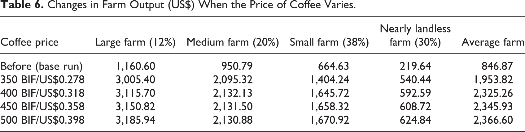
With all other factors kept constant, any change in crop prices is likely to affect the composition of farm output itself and the market value of the total production. Table 6 shows the values of farm output with changing coffee prices in scenario I. In the base run, coffee is not selected in the model. However, when the price increases by as little as 50 BIF (US$0.04) per kilogram, coffee enters into the model and the overall output increases considerably for all farm categories.

Table 6.

Changes in Farm Output (US$) When the Price of Coffee Varies.

Coffee price	Large farm (12%)	Medium farm (20%)	Small farm (38%)	Nearly landless farm (30%)	Average farm
Before (base run)	1,160.60	950.79	664.63	219.64	846.87
350 BIF/US$0.278	3,005.40	2,095.32	1,404.24	540.44	1,953.82
400 BIF/US$0.318	3,115.70	2,132.13	1,645.72	592.59	2,325.26
450 BIF/US$0.358	3,150.82	2,131.50	1,658.32	608.72	2,345.93
500 BIF/US$0.398	3,185.94	2,130.88	1,670.92	624.84	2,366.60

The model is also very sensitive to the price of bananas. Because 93.3% of households get their income from selling both banana beer or wine and plantains, any change in the banana market could affect the livelihoods of many families. Table 7 depicts the trends in farm outputs when the price of bananas changes.

Table 7.

Changes in Farm Output (US$) When the Price of Bananas Varies (scenario I).

Change in banana price	Large farm (12%)	Medium farm (20%)	Small farm (38%)	Nearly landless farm (30%)	Average farm
Before (base run)	1,160.60	950.79	664.63	219.64	846.87
210 BIF/US$0.167	3,005.40	2,095.32	1,404.24	540.44	1,953.82
250 BIF/US$0.199	3,005.72	2,095.32	1,404.24	540.44	1,953.82
280 BIF/US$0.223	3,141.97	2,146.88	1,408.85	543.12	2,000.48
300 BIF/US$0.239	3,270.54	2,201.90	1,429.92	555.41	2,092.88

Empirical Validation of the Predictions of the Model

Given the local prices for agricultural commodities in 2010, the model predicts that rational households should shift their production pattern over time toward the most profitable crops. However, changing production patterns is a difficult decision and often requires costly investment because uprooting and replanting of certain crops is necessary. Hence, even if households are completely rational and base their decisions only on the variables included in the model (land, availability of labor and fertilizer, and price and nutritional value of the different crops), production patterns will change only slowly over time.

2In addition, households can opt to change production along extensive or intensive margins that are not strictly determined by the model. In the former, it is assumed that fields devoted to the most profitable crops are expanded at the expense of fields previously used for production of the least profitable crops. In the latter, households choose to target the scarce resources (labor and fertilizer) toward the most profitable crops but do not expand the area devoted to these crops. Generally, changes at the extensive margins will require more time than changes along the intensive margins because there are higher fixed costs involved.

Our detailed panel dataset with 340 observations covers a time span of 5 years (2007–12), which is arguably sufficient to investigate whether agricultural production indeed shifted over time toward the crops predicted by the model. The fact that the estimation of technical coefficients was based on data collected in 2010 does not imply that this shift should only have started in 2010, because the characterization of the different farm types was based on data collected in 2007. We assume, therefore, that the prediction of the model should be valid for the period from 2007 to 2012.

Table 8 shows the changes in agricultural production for the main crops between 2007 and 2012. For both years, the number of households growing a particular crop and the average production per household conditional on cultivating that crop are given. The former is a proxy for the extensive margin, because if more households planted a particular crop in 2012 than in 2007, some households must have decided to devote at least one new field to this crop. The second variable is a proxy for both the intensive and the extensive margins, because households can increase production by increasing the area assigned to a particular crop, increasing labor efforts, or using other inputs, such as fertilizer.

Table 8.

Changes in Production of the Main Crops Between 2007 and 2012.

Crop	2007		2012		2007–2012 change
Crop	Average production (kg)	% of households growing crop	Average production (kg)	% of households growing crop	2007–2012 change
Bananas	2,084	95	3,190	98	– 894***
Beans	145	95	254	98	109***
Cassava	461	62	389	59	– 72
Coffee	439	63	258	55	– 181***
Groundnuts	63	8	50	11	– 13
Peas	24	15	24	26	0
Potatoes	225	41	284	40	– 59
Rice	177	39	159	45	– 18
Sweet potatoes	1,050	92	880	95	– 170***

***p < .01, **p < .05, *p < .10, t-test with unequal variance.

It is remarkable that the average production of beans per farm increased considerably from 145 kg in 2007 to 254 kg in 2012, while the number of households that cultivated beans also increased slightly. In both 2007 and 2012, more than 95% of households cultivated beans, which is one of the main staple crops in the Burundian diet. These results are in line with the model. In both scenarios I and II, the model predicts that households should specialize in bean production because this crop has a high price and nutritional value and can be grown efficiently.

The average production of cassava and groundnuts decreased between 2007 and 2012, although the changes are not significant at a 10% level of statistical significance. This change contradicts the findings of the model, because cassava production was expected to increase according to scenario I and groundnut production was expected to increase according to scenario II, in which all households cultivate groundnuts because of their high nutritional value.

According to the model, the production of sweet potatoes and peas is not profitable for any of the farm types, while the production of potatoes is only profit maximizing for small and nearly landless farmers in scenario I. Between 2007 and 2012, sweet potato production declined significantly, but it remained a very important staple crop for most households, with an average production of 880 kg in 2012. Hence, this marked reduction is in line with the model. The production of potatoes, however, remained stable, while the proportion of households that cultivated peas increased from 15% to 24%.

Total rice production remained stable between 2007 and 2012, but the proportion of households cultivating rice increased from 39% to 45% and the average production per household decreased slightly. This result is also not surprising, because rice can only be cultivated in some parts of the wetlands and the scope for an increase in production is therefore limited. Wetland is not considered in the model as a separate input for rice production. This explains why, according to scenario I, all households should increase rice production, which is probably not feasible in the short run given the nonavailability of irrigation. We should recognize this as a clear limitation of our model. Additional properties and constraints, such as soil quality and access to water, should be added to account for the limited potential of rice production. We also might speculate that the profitability of rice production, as predicted by the model, increases the competition for the wetland suitable for rice production. It is worth noting that land allocation in wetlands is based on a complex traditional governance system.

Banana production decreased dramatically between 2007 and 2012. This is probably not due to farmers' choice, but rather it may be the effect of the Xanthomonas wilt that affected banana trees in the region.³¹

Coffee production in Burundi is biannual, with an excellent harvest in 2007 and a bad harvest in 2012, which makes interpretation of the reduction in average coffee production between 2007 and 2012 difficult.³² There is, however, some suggestive and anecdotal evidence that farmers reduced the number of coffee trees and are no longer willing to invest in new trees because of the low local prices. In our sample, the number of households that cultivated coffee decreased from 198 in 2007 to 174 in 2012.

A second way to assess whether the households indeed behaved as predicted by the model is to investigate which crops were planted on fields newly acquired between 2007 and 2012. New fields often need extra initial investment and are initially more labor intensive than fields that have been in the household for a long time. It is therefore reasonable to assume that a household will only be willing to buy fields and invest time, money, and energy in these new fields if they are certain to make a profit over time. Table 9 shows which crops were planted on the newly acquired fields.

Table 9.

Main Crops Planted on New Fields.

Crop	%
Beans	31
Cassava	28
Bananas	15
Reforestation	8
Coffee	7
Other	11

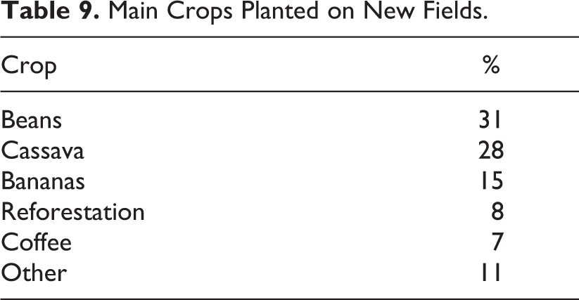
Eighty-seven households bought at least one new field between 2007 and 2012. These fields were mainly used to cultivate beans (31%), cassava (28%), and bananas (15%). Only 7% of the households planted coffee on these new fields or might have bought them already bearing coffee trees. The choice of beans and cassava corroborates the model predictions.

The empirical evidence that confirms the reliability of the model is therefore mixed. The increase in bean production, the decrease in sweet potato and coffee production, and the choice of crops for new fields are in line with the predictions of the model. However, the limited decrease in cassava and potato production and the increase in pea production were not predicted by the model.

Conclusions and Perspectives

Like most African countries, Burundi’s agricultural sector is mainly dominated by small-scale farmers. These farmers produce for subsistence purposes on highly fragmented lands using very little input. Yet, the low input level, lack of market orientation, and limited exchanges between farms have negatively affected land and labor productivity. With current farm practices, more than half of the farming population is unable to satisfy their household food needs. Moreover, the options for diversification of livelihoods through agriculture for these small farms are very low and are limited to low-paid irregular jobs on other people’s farms or businesses. This has led to a rapid deterioration of the country’s food security situation.

Nevertheless, despite the rampant land scarcity, our models show that it is still possible for households to find optimal crop combinations that could meet minimal food security requirements while generating a certain level of income, except for nearly landless households. By growing specific ranges of crops, farmers can benefit from an optimal land use that further contributes to improved farm output and to rising opportunity costs of family labor. At the optimal level of production, farmers with different resources and capabilities are likely to adopt different activities. By producing crops in which the farms have comparative advantages and trading, large and medium farms can improve their productivity and hire extra workers to supplement family labor. On the other hand, the model highlighted that the optimum resource combination for agricultural production was not possible for nearly landless farms. They have to rely on the labor market to fulfill household basic needs. Therefore, any policy for improving off-farm activities and the labor market might improve the living conditions in these farms with a limited access to land.

The implications of our results are that at the local level, there is scope for specialization, improved farm output, and more intrarural exchanges between farms. According to Hazell and Wood³³, as per capita incomes rise, labor becomes more expensive relative to land and capital, and small farms may get squeezed out by larger and more capitalized farms that become better placed to compete. Therefore, small and nearly landless farms should exploit their comparative advantages (available labor in the household) and benefit from the increasing off-farm employment opportunities.

Agricultural specialization is a potential way of successfully overcoming poverty and hunger in the community. Conditions necessary for agricultural specialization include market infrastructure, improved storage facilities, credit, and agricultural research. These conditions require profound adjustments in both production processes and policy-making. Therefore, further research should integrate institutions and production policies in a multiagent-based model to explore agricultural policy options in the near future for optimizing the farming plans and household living standards in Burundi.

There are several aspects linked to institutional or/and failing markets that influence the choice of a particular crop that were not included in the model but that nevertheless play an important role. First, some input variables, such as the access to wetland for rice production, were not included in the model. Similarly, other inputs, such as organic fertilizer, which contributes significantly to soil fertility in Burundi, could not be included due to difficulties in measuring the input needs.¹⁷ Second, the results of the model are based on 2010 prices, which may have changed over the years, and on estimated technical coefficients for the production of the different crops, which may not be invariable over time, as production techniques or environmental constraints may have changed. Third, even rational households might be unable to choose the most productive crops due to a lack of knowledge and extension work. The possibility of experimenting with different cropping systems is limited in Burundi, because the risk involved in such experiments is too high for households that barely survive. Fourth, households not only may be profit maximizing, but may try to reduce the risk of acute hunger and, hence, avoid crops that are vulnerable to weather conditions. These are areas of further research.

Although the model has several flaws due to simplification of reality, it is surprising that a straightforward model yields remarkably accurate results and enables the prediction of some general trends in farmers’ decision-making on crop choices. The model seems to predict rather accurately how farmers choose crops that are either of high market or high nutritional value, or that are relatively undemanding in terms of inputs. Even in the absence of specific specialization policies and in the presence of food insecurity and risk, farmers seem to act as optimizing agents. More detailed optimization models are therefore a valuable tool to investigate the main bottlenecks to agricultural production and to investigate the opportunities for increased specialization between farm types.

Footnotes

Supplemental Material

A supplemental appendix to this article is published electronically only at .

Declaration of Conflicting Interests

The author(s) declared no potential conflicts of interest with respect to the research, authorship, and/or publication of this article.

Funding

The author(s) disclosed receipt of the following financial support for the research, authorship, and/or publication of this article: The authors acknowledge the financial support from the Belgian inter-university cooperation project (ZEIN2007PR336-69525) between Belgian (Flemish) Universities and the University of Burundi (VLIR-UOS).

References

Haddad

. From nutrition plus to nutrition driven: How to realize the elusive potential of agriculture for nutrition? Food Nutr Bull 2013;34:39–44.

Turner

Hawkes

Waage

Ferguson

Haseen

Homans

Hussein

Johnston

Marais

Mcneill

Shankar

. Agriculture for improved nutrition: The current research landscape. Food Nutr Bull 2013;34:369–77.

World Bank. World development report 2008: Agriculture for development. Washington, DC: World Bank, 2007.

Cunguara

Darnhofer

. Assessing the impact of improved agricutural technologies on household income in rural Mozambique. Food Policy 2011;36: 378–90.

Fulginiti

Perrin

Bingxin

. Institutions and agricultural productivity in Sub-Saharan Africa. Agric Econ 2004;31:169–80.

Savadogo

Reardon

Pietola

. Adoption of improved land-use technologies to increase food security in Burkina Faso: Relating animal traction, productivity, and nonfarm income. Agric Syst 1998;58:441–64.

Timmer

. Farmers and markets: The political economy of new paradigms. Am J Agric Econ 1997;79:621–7.

Adesina

. Conditioning trends shaping the agricultural and rural landscape in Africa. Agric Econ 2010;41:73–82.

Nkala

Mango

Corbeels

Velduisch

Huising

. The conundrum of conservation agriculture and livelihoods in Southern Africa. Afr J Agric Res 2011;6:5520–8.

10.

Kaimonwitz

Angelsen

. Economic modes of tropical deforestation. A review. Jakarta: Center for International Forestry Research, 1998.

11.

Lambin

Rounsevell

MDA

Geist

. Are agricultural land use models able to predict change in land-use intensity? Agric Ecosyst Environ 2000;82:321–31.

12.

Verschelde

D’Haese

Rayp

Vandamme

. Challenging small scale farming: A non parametric analysis of the (inverse) relationship between farm productivity and farm size in Burundi. J Agric Econ 2012;11:261–87.

13.

Ministère de l’Agriculture et de l’Elevage. Stratégie Agricole Nationale 2008-2015. Bujumbura, Burundi: Ministère de l’Agriculture et de l’Elevage, 2008.

14.

World Food Programme. Food security and vulnerability analysis. Rome, Italy: World Food Programme, 2004.

15.

Baghdadli

Harborne

Rajadel

. Breaking the cycle: A strategy for conflict-sensitive rural growth in Burundi. Washington, DC: World Bank, 2008.

16.

Bergen

. Perspectives de la spécialisation régionale comme stratégie de développement. Synthèse nationale des dossiers par région naturelle sur les flux des produits agricoles. Bujumbura, Burundi: Institut des Sciences Agronomiques du Burundi, 1986.

17.

Cochet

. Agrarian dynamics, population growth and resource management: The case of Burundi. GeoJournal 2004;60:111–22.

18.

Rishirumuhirwa

Roose

. The contirbution of banana farming systems to sustainable land use in Burundi. Adv Geoecol 1998;31:1197–204.

19.

D’Haese

Speelman

Vandamme

Nkunzimana

Ndimubandi

D’Haese

. Recovering from conflict: An analysis of food production in Burundi, S.A. Paper presented at AAAE and AEASA Conference, September 2010.

20.

Banderembako

. The link between land, environment, employment, and conflict in Burundi. Bujumbura, Burundi: US Agency for International Development, 2006.

21.

Ahishakiye

. Influence of agricultural production techniques on food security in Burundi: A case study of Ngozi. Master’s dissertation, Ghent University, 2011.

22.

MPDRN. Monographie du Burundi. République du Burundi, Bujumbura, Burundi; 2006.

23.

Pender

Ruben

. Rural diversity and heterogeneity in less favourable areas: The quest for policy targeting. Food Policy 2004;29:303–20.

24.

Köbrich

Khan

TRM

. Typification of farming systems for constructing representative farm models: Two illustrations of the application of multi-variate analysis in Chile and Pakistan. Agric Syst 2003;76:141–57.

25.

Manyong

Degand

D’Haese

Ndimira

. Research on a typology of traditional farming in Burundi. Agric Syst 1987;28:103–17.

26.

Havard

Bessane

Nana

Djonnewa

Djondang

Leroy

. Typologies des exploitations agricoles dans les savanes d’Afrique centrale: Un regard sur les methodes utilisées et leur utilité pour la recherche et le développement. Garoua, Cameroun: Actes du Colloque, 2002.

27.

Buysse

Huylenbroeck

Lauwers

. Normative, positive and econometric mathematical programming as tools for incorporation of multifunctionality in agricultural policy modeling. Agric Ecosyst Environ 2007;120:70–81.

28.

Glen

Tipper

. A mathematical programming model for improvement planting in a semi-subsistence farm. Agric Syst 2001;70:295–317.

29.

Ndimira

. Dynamique et problématique d’amélioration des systèmes d’exploitation agricoles au Burundi. Cas de Remera. Louvain-La-Neuve, Belgium: Université Catholique de Louvain, 1991.

30.

Latham

. La nutrition dans les pays en développement. Rome: Food and Agriculture Organization, 2001.

31.

Tripathi

. Relative susceptibility of banana cultivars to Xanthomonas campestris pv. Musacearum . Afr J Biotechnol 2009;8:5343–50.

32.

International Coffee Organization. Historical data of total production. Available at: http://www.ico.org/new_historical.asp. Accessed 7 April 2015.

33.

Hazell

Wood

. Drivers of change in global agriculture. Phil Trans B 2008;12:495–515.

Supplementary Material

Please find the following supplemental material available below.

For Open Access articles published under a Creative Commons License, all supplemental material carries the same license as the article it is associated with.

For non-Open Access articles published, all supplemental material carries a non-exclusive license, and permission requests for re-use of supplemental material or any part of supplemental material shall be sent directly to the copyright owner as specified in the copyright notice associated with the article.

0.00 MB

0.08 MB