Route-Constrained Optimization Models for Electric School Bus Allocation and Stop Sequencing

Abstract

This study underscores the growing need to transition from conventional school buses powered by internal combustion engines to electric school buses (ESBs). We propose mixed integer programming (MIP)-based approaches to optimize the allocation of ESBs to predetermined routes while determining their travel paths and bus stop sequences. The problem formulation incorporates heterogeneous ESBs with mixed student loading. Essential factors such as bus seating capacity, battery capacity, energy consumption cost, and procurement cost are considered to determine optimal bus selection and allocation strategies that minimize total expenses. To address this challenge, we introduced two methodologies: a MIP-based optimization model and a two-stage hybrid model that integrates optimization with heuristic approaches. We evaluate the efficiency of the proposed approaches through nineteen computational scenarios and compare their performance. The results indicate that the hybrid model significantly improves computational efficiency for large-scale problem instances, demonstrating its potential as a scalable tool for strategic planning.

Keywords

electric school bus heuristic routing mixed integer programming optimization

Introduction

Despite the growing adoption of electric vehicles (EVs) in public transit networks globally, the overall transportation sector remains heavily dependent on internal combustion engine vehicles (ICEVs), which primarily rely on fossil fuels. This dependence has substantial environmental implications, including air pollution and adverse health effects caused by emissions such as carbon monoxide, nitrogen oxides, and particulate matter. Furthermore, ICEVs are major contributors to greenhouse gas emissions, particularly carbon dioxide (CO₂), which accelerates climate change, leading to extreme weather conditions and rising sea levels. According to the United States Environmental Protection Agency ( 1 ), transportation accounted for 38.1% of CO₂ emissions and 28.9% of total greenhouse gas emissions from fossil fuel combustion in the United States in 2022.

Apart from emissions, the extraction, refinement, and transportation of fossil fuels exacerbate environmental degradation through habitat destruction, water contamination, and ecosystem disruption. Additionally, improper disposal of used motor oil and other automotive waste further threatens soil and water quality. Given these environmental concerns, transitioning to cleaner and more sustainable transportation solutions has become imperative.

EVs have emerged as a promising alternative, offering zero tailpipe emissions and improved air quality, especially when charged using renewable energy sources such as wind, hydro, or solar power. EV technology continues to advance, with innovations such as regenerative braking enhancing energy efficiency ( 2 ). Although EVs were first introduced in the late 19th century, their adoption was limited because of constraints in battery technology, driving range, and charging infrastructure. However, renewed concerns about energy security, pollution, and climate change have reinvigorated interest in EVs. Technological improvements have extended their range and reduced charging times, while government incentives and automaker investments have made EVs more cost-effective and accessible. Fluctuating fuel prices and declining EV costs have further encouraged consumer adoption.

One significant application of EV technology is in school transportation. In the United States, over 25 million students rely on approximately 500,000 school buses daily, with most of these buses powered by diesel engines. Diesel exhaust has been linked to respiratory issues and can negatively affect children’s health and academic performance. Studies indicate that diesel fumes can impair lung function by reducing epithelial cell membrane potential ( 3 ). For this reason, school districts in many regions, particularly in North America, are transitioning to electric school bus (ESB) fleets, a move driven by environmental benefits, reduced noise pollution, and potential long-term operational cost savings. However, as of early 2024, data from the World Resources Institute indicate that although commitments are increasing, ESBs still represent less than 2% of the approximately 480,000 school buses in the United States ( 4 ). The vast majority of the fleet continues to rely on diesel, contributing significantly to local air pollution and greenhouse gas emissions. This transition, however, presents significant logistical and financial challenges.

In traditional school bus fleets, vehicle range is rarely a limiting factor. A diesel bus can typically travel over 500 mi on a single tank, which far exceeds the requirements of any daily route. Consequently, any bus in a diesel fleet can, in theory, serve any route. This makes the range constraint mathematically redundant in most assignment scenarios.

In contrast, ESBs often have ranges of 80 to 120 mi. This is critically close to daily travel requirements and turns vehicle range from a safety margin into a hard constraint that dictates feasibility. This introduces a strategic fleet sizing challenge distinct from diesel operations. Unlike the uniform diesel market, the electric bus market requires operators to choose between vehicles with varying battery capacities and significantly different capital costs. An optimization model is therefore required to solve this heterogeneous asset-matching problem. It ensures that higher-cost, long-range buses are procured only for routes that strictly require them, while shorter routes are served by more cost-effective units. Standard vehicle routing problem (VRP) algorithms often assume that all vehicles have uniform range capabilities or unlimited fuel access. Therefore, they cannot adequately address the trade-off between capital cost and range capability that is central to electrifying a fleet.

The models presented in this paper are designed primarily for transportation planners in school districts with dedicated, fixed-route systems, a common operational paradigm in the United States. They are intended as a strategic planning tool to aid in the initial phase of fleet electrification, focusing on the critical decisions of which buses to procure and how to assign them to existing routes to minimize total long-term cost. This research differs from other routing studies because of its route-constrained characteristics. Unlike most routing research, which allows greater flexibility in selecting locations and determining bus stop placements, our model adheres to fixed bus stops and predetermined routes, closely mirroring real-world operational constraints for districts not looking to overhaul their existing networks.

This paper presents a significant extension of our preliminary work, which introduced the initial model concepts ( 5 ). Here, we provide a more detailed mathematical formulation, introduce a novel hybrid heuristic model (HAS), and conduct a comprehensive computational study across nineteen scenarios, including a thorough sensitivity analysis, to rigorously evaluate the performance and scalability of our approaches. The main contribution of this work is methodology: we propose and compare an exact optimization model (MIP-AS) with a scalable hybrid heuristic (HAS) to solve the integrated ESB allocation and sequencing problem, demonstrating the computational trade-offs and highlighting the hybrid approach’s efficiency for large-scale strategic planning.

The rest of this paper is organized as follows: The next section provides a review of relevant literature on school bus routing and EV scheduling. The problem definition and the key challenges addressed in this study are then presented. Following this, a section details the proposed methodologies, discusses model development, and evaluates computational results. The final section concludes with key findings and directions for future research.

Literature Review

Vehicle routing and scheduling have been extensively studied, with school bus routing emerging as a crucial subdomain. Research in this area is broadly categorized into public transportation routing and school bus routing. The School Bus Routing Problem (SBRP) is distinct from general public transit because of its specific operational nature: routes are designed to transport a defined set of students from various locations to a central destination (the schools) without intermediate drop-offs, and adhere to maximum ride-time limits for student welfare. This differs fundamentally from public transit, where passengers board and alight dynamically at any stop along the network. This section reviews existing work on school bus allocation, routing, and scheduling, before discussing the specific challenges of electric fleet sizing and assignment. The SBRP encompasses multiple sub-problems, including bus stop selection, route generation, scheduling, school bell time adjustments, and strategic policy considerations ( 6 ). Some studies tackle these sub-problems individually, whereas others integrate them for a holistic approach.

For instance, Sarubbi et al. ( 7 ) introduced a heuristic algorithm for student-to-bus stop assignments, minimizing the number of stops while maintaining acceptable walking distances. Riera-Ledesma and Salazar-González ( 8 ) used a column generation algorithm to optimize bus stop selection based on constraints such as minimum student capacity per stop and maximum walking distances. Schittekat et al. ( 9 ) proposed a metaheuristic model that simultaneously optimizes stop selection and route generation, whereas Calvete et al. ( 10 ) developed a two-stage metaheuristic approach to reduce travel costs and walking distances. Sciortino et al. ( 11 ) presented a heuristic model incorporating heterogeneous fleets, multiple stops, and varying walking distance constraints.

Beyond stop selection, researchers have examined operational policies to further optimize fleet utilization. One such policy is “mixed loading,” where a single bus transports students from multiple schools simultaneously. Ellegood et al. ( 12 ) highlighted the efficiency gains of mixed loading in large districts where schools often share catchment areas. Yao et al. ( 13 ) expanded on this by proposing routing strategies that utilize virtual stops and interscholastic transportation. Furthermore, Shang et al. ( 14 ) demonstrated that integrating mixed loading with heterogeneous fleets and variable time windows can significantly enhance routing flexibility, an approach that aligns with the multi-school service model adopted in this study.

Strategic adjustments to school operating hours have also been explored as a method to reduce fleet requirements. Bertsimas et al. ( 15 ) demonstrated that optimizing school bell times could lead to substantial cost savings, a method successfully implemented in the Boston public school system. Qian ( 16 ) further advanced this domain by applying multicriteria optimization to identify optimal start times. Although our study focuses on fixed bell times, these findings underscore the interconnectedness of scheduling policy and fleet efficiency.

Time-dependent factors have also been integrated into routing studies. Orejuela and Hernandez ( 17 ) developed a routing system that accounts for variable travel times based on departure schedules. Hou et al. ( 18 ) optimized bus routing for heterogeneous fleets under unlimited and limited fleet conditions, minimizing fixed and variable costs using a hybrid metaheuristic algorithm. Similarly, Ansari et al. ( 19 ) formulated a mathematical model to enhance the routing efficiency of special needs students, validated through real-world applications in Fort Smith, Arkansas. Shafahi et al. ( 20 ) proposed a mixed-integer programming model and a matching-based heuristic to solve the “balanced” school bus scheduling problem, which aims to create tours of similar length to avoid overtime charges. Their heuristic approach was able to find reasonable solutions in a much shorter time than commercial solvers, saving up to 16% in operation costs in some scenarios.

Although most studies focus on traditional diesel school buses, limited research exists on ESB routing, scheduling, and allocation. However, studies on EV routing provide valuable insights into managing constraints related to battery range, charging infrastructure, and operational costs. Li and Chow ( 21 ) address the routing of special education and general education students, proposing a “mixed ride” system where both student types can be on the same bus. Their approach, which uses a heterogeneous fleet and allows for mixed student loads, showed a 14.32% reduction in total travel distance and a 10.46% reduction in total travel time in a New York City case study. Hulagu and Celikoglu ( 2 ) developed a mixed integer programming (MIP)-based model to optimize university shuttle fleet routing, considering operational and charging costs. Taş ( 22 ) introduced an Electric Vehicle Routing Problem with Flexible Time Windows, balancing travel schedules with penalty costs for early or late arrivals. Lu et al. ( 23 ) formulated a time-dependent EV routing model that integrates congestion, time windows, vehicle capacity, and battery recharging limitations. Basso et al. ( 24 ) addressed a time-dependent EV routing problem with chance constraints, incorporating partial recharging to optimize routes under uncertainty. Zhang et al. ( 25 ) proposed a MIP model for multi-depot EV scheduling, optimizing transit routes while considering parking restrictions and partial recharging.

Although optimizing routes is a well-studied problem, the transition to EVs introduces significant upfront capital costs and new operational constraints, elevating the strategic importance of fleet planning. The core contribution of this paper lies in fleet sizing and assignment decision-making rather than novel route generation. This aligns our work with several key research streams.

First, our problem is a variant of the Electric Fleet Size and Mix Vehicle Routing Problem (E-FSMVRP), formally defined by Hiermann et al. ( 26 ). In the E-FSMVRP, the objective is not only to route vehicles but to simultaneously determine the optimal composition of the fleet (e.g., battery sizes, seating capacities) to minimize total costs. Our model adopts this principle by selecting from a list of available ESB models with different specifications to meet the route demands.

Second, recent research emphasizes that battery capacity and charging constraints are the primary drivers of Total Cost of Ownership (TCO) for electric bus fleets. Rogge et al. ( 27 ) demonstrated that optimizing fleet composition alongside charging infrastructure is essential for minimizing TCO, as fixed battery sizes may not be optimal for all routes. Similarly, Yıldırım and Yıldız ( 28 ) highlighted that efficient fleet composition can significantly reduce procurement costs by matching specific vehicle capabilities to schedule requirements.

Finally, within the specific domain of school transportation, Li and Chow ( 21 ) explored the benefits of deploying a heterogeneous fleet with mixed loads. Their work confirms that moving away from a homogeneous fleet assumption allows for significant efficiency gains. As categorized in the comprehensive review by Perumal et al. ( 29 ), our work sits at the intersection of strategic fleet sizing and tactical assignment. By integrating procurement costs directly into the optimization objective, our MIP-AS model provides a tool for the high-level decision-making required during the initial phase of fleet electrification.

Although there have been significant advancements in general school bus routing and EV routing, research addressing the strategic fleet planning challenges of ESBs remains scarce. The constraints imposed by battery capacity, fleet heterogeneity, and high procurement costs necessitate innovative allocation and sequencing strategies tailored specifically to ESBs. This study bridges this research gap by developing a hybrid optimization model that effectively sizes and allocates ESB fleets while optimizing travel sequences to enhance efficiency and cost-effectiveness.

Problem Definition

This study aims to develop models for efficiently assigning ESBs to established routes that are currently serviced by conventional school buses powered by internal combustion engines. The models presented in this paper are designed primarily for transportation planners in school districts with dedicated, fixed-route systems. It is intended as a strategic planning tool to aid in the initial phase of fleet electrification, focusing on the critical decisions of which buses to procure and how to assign them to existing routes to minimize total long-term cost. The objective is to optimize the travel paths of ESBs to transport students while minimizing costs associated with procurement and charge consumption.

This research differs from other routing studies because of its route-constrained characteristics. Unlike most routing research, which allows greater flexibility in selecting locations and determining bus stop placements, our model adheres to fixed bus stops and predetermined routes, closely mirroring real-world operational constraints for districts that wish to electrify their fleet without completely overhauling their existing route network. Consequently, this study is limited to utilizing existing bus stops for each designated route to determine the ESBs’ travel paths.

Our model relies on several necessary operational assumptions to make the strategic fleet sizing problem tractable. First, we assume a fixed assignment where each route is served by a single, dedicated bus. This is a common approach in strategic planning, especially during an initial fleet transition, to simplify operations and ensure reliable service for each established route. Second, concerning student loading, we assume a morning-route scenario where all students are picked up along the route before any drop-offs occur at the schools. Consequently, the capacity constraint requires the selected bus to have a seating capacity sufficient for the total number of students on its assigned route. This represents a worst-case loading scenario; while this simplifies the formulation, it provides a conservative and robust allocation, ensuring capacity is never an issue. Finally, with regard to charging logic, this study does not factor in recharging schedules or the location of charging stations, as school buses typically have extended idle times, allowing for recharging on returning to the terminal. Therefore, the constraint focuses on ensuring the battery range is sufficient for a complete round trip without intermediate charging.

This paper introduces an efficient model for allocating ESBs and sequencing pre-determined routes currently used by conventional school buses. It considers various ESB types and the mixed loading of students from different schools. Key factors such as seating capacity, battery capacity, and bus pricing are incorporated into the allocation process to enhance cost-effectiveness. Additionally, this study does not factor in recharging schedules or the location of charging stations, as school buses typically have extended idle times, allowing for recharging on returning to the terminal. Furthermore, all input data, including stop-to-route assignments, distances, and student numbers, were randomly generated to simulate realistic problem scenarios. This approach was adopted to create a broad set of test scenarios that emulate realistic conditions while enabling a scalable and flexible evaluation of the model’s algorithmic performance.

Proposed Computational Approaches

This section discusses two different computational approaches designed to solve the same problem. Both approaches aim to determine which bus will travel to which location and the sequence of travel for each route. They allow for mixed loading, meaning students from different schools can share a bus. The models also take into account a list of different ESBs with specific seating capacity, battery capacity, and prices available for selection. Both models assume that each bus will be assigned to only one route and that each route should have a single bus. The allocation process is not affected by school bell times. It is also assumed that all buses start their routes fully charged from the terminal and are recharged only on returning after completing student drop-offs. These models do not account for intermediate charging because of the ample idle time available for school buses. Additionally, the models consider a uniform rate for electricity consumption during the trips. Furthermore, these models consider the number of students in each location, locations in a specific route, and the distance between locations as input.

It is important to note that this study utilizes randomly generated datasets. This approach was deliberately chosen to test the algorithmic performance and scalability across a wide spectrum of problem sizes and structures, ranging from small to very large-scale instances. This allows for a robust evaluation of the computational limits of the proposed models, a primary objective of this methodological paper. Validation against a real-world case study from a specific school district is an important next step to assess the model’s practical performance and is a key direction for future research.

Allocation and Sequencing Optimization Model

We have developed an MIP-based Allocation and Sequencing (MIP-AS) optimization model for allocating ESBs to predetermined routes and sequencing student stops on these existing routes that had been assigned conventional school buses powered by internal combustion engines. The objective of the MIP-AS model is to minimize the overall cost of purchasing and charging ESBs while satisfying ESBs’ seating and battery capacities.

MIP-AS Model Formulation

All the necessary notations needed to formulate the model are introduced in Table 1. We assume that all input parameters are deterministically identified.

Table 1.

Notations for MIP-AS Optimization Mode

Notation	Description	Type/use
R	Set of routes.	S
$\| R \|$	The cardinality of set R.	IP
r	Index of routes.	I
B	Set of buses.	S
b	Index of buses.	I
L	Set of locations.	S
L ^S	Set of schools which is a subset of L.	S
L ^L	Set of bus stops which is a subset of L.	S
L ^T	Set of all bus stops and schools (i.e., all locations except the terminal) L.	S
l & k	Index of location.	I
S _b	Seating capacity of bus b.	IP
F _b	Battery capacity of bus b in kWh.	IP
W _rl	It is 1 if location l is included in route r and 0 otherwise.	IP
N _rl	The number of students in location l for route r.	IP
D _lk	Distance between location l and k.	IP
P _b	Price of bus b.	IP
C	Cost of charging per kWh.	IP
E	Required battery capacity to travel per mile.	IP
M	Arbitrary big number.	IP
Tw	Time window/ time limit for each bus to complete one trip (in minutes).	IP
X _br	Binary variable is 1 if bus b is allocated to route r and 0 otherwise.	DV
A _b	Binary variable is 1 if bus b is allocated to any route and 0 otherwise.	DV
U _rl	Positive variable used for detour elimination.	DV
V _brlk	Binary variable is 1 if bus b allocated to route r is going from location l to location k and 0 otherwise.	DV

Note: MIP-AS = Mixed Integer Programming Allocation and Sequencing; S = set; I = index; IP = input parameter; DV = decision variable.

Objective function:

\begin{matrix} Min ((\sum_{b = 1}^{B} P_{b} A_{b}) / 12.5) \\ + (2 C ((\sum_{b = 1}^{B} \sum_{r = 1}^{R} \sum_{l = 1}^{L} \sum_{k = 1}^{L} V_{brlk} D_{lk}) E 180)) \end{matrix}

(1)

Subject to:

\sum_{r = 1}^{R} X_{br} \leq 1 for \forall b \in B

(2)

\sum_{l = 1}^{L} \sum_{k = 1}^{L} V_{brlk} \leq M A_{b} for \forall b \in B and r \in R

(3)

\sum_{b = 1}^{B} \sum_{r = 1}^{R} V_{brll} = 0 for \forall l \in L

(4)

\sum_{b = 1}^{B} \sum_{k = 1}^{L} V_{brlk} = W_{rl} for \forall r \in R and l \in L^{T}

(5)

\sum_{b = 1}^{B} \sum_{l = 1}^{L} V_{brlk} = W_{rk} for \forall r \in R and k \in L^{T}

(6)

\sum_{l = 1}^{L} \sum_{k = 1}^{L} V_{brlk} \leq M X_{br} for \forall b \in B and r \in R

(7)

\sum_{k \in L^{L}} V_{brl 1 k} W_{rk} = X_{br} for \forall b \in B and r \in R

(8)

\sum_{b = 1}^{B} \sum_{r = 1}^{R} \sum_{l \in L^{S}} \sum_{k \in L^{L}} V_{brlk} = 0

(9)

\sum_{b = 1}^{B} \sum_{l \in L^{L}} \sum_{k \in L^{S}} V_{brlk} = 1 for \forall r \in R

(10)

\sum_{b = 1}^{B} \sum_{k \in L^{S}} V_{brkl 1} = \sum_{b = 1}^{B} X_{br} for \forall r \in R

(11)

\sum_{r = 1}^{R} \sum_{b = 1}^{B} V_{brlk} + \sum_{r = 1}^{R} \sum_{b = 1}^{B} V_{brkl} \leq 1 for \forall l \in L^{T} and k \in L^{T}

(12)

\begin{matrix} \sum_{r = 1}^{R} (U_{rl} - U_{rk} \sum_{b = 1}^{B} (card (L^{L}) V_{brlk})) \leq card (L^{L}) \\ - 1 for \forall l \in L^{L} and k \in L^{L} \end{matrix}

(13)

\sum_{k = 1}^{K} V_{brlk} = \sum_{k = 1}^{K} V_{brkl} for \forall b \in B, r \in R and l \in L

(14)

\sum_{l = 1}^{L} \sum_{k = 1}^{L} V_{brlk} N_{rl} \leq S_{b} for \forall b \in B, r \in R

(15)

(\sum_{l = 1}^{L} \sum_{k = 1}^{L} V_{brlk} D_{lk} M) \leq Tw * X_{br} for \forall b \in B and r \in R

(16)

2 E (\sum_{l = 1}^{L} \sum_{k = 1}^{L} V_{brlk} D_{lk}) \leq F_{b} * X_{br} for \forall b \in B, r \in R

(17)

In this MIP-AS optimization model, Equation 1 represents the objective function, which aims to minimize the total procurement cost of buses and the total electricity consumption cost. The first part of the objective function indicates the annual depreciated procurement costs of the ESBs considering their average 12.5-year lifespan. On the other hand, the second part indicates the cost of yearly electricity consumption by the ESBs, considering the 180-day school year. Equations 2 to 17 represent the constraints for the MIP-AS optimization model. Constraint (2) ensures that no bus will be assigned to more than one route. Constraint (3) confirms if a bus is allocated to any route. Constraint (4) prevents travel from and to the same location. Constraints (5) and (6) ensure that a bus selected for a route will travel from one location to another by only one path. Constraint (7) prevents a bus from visiting any location that is not included in the route to which the bus is assigned. Constraint (8) indicates that all the assigned buses will start their trip to any route from terminal (l₁). Constraint (9) guarantees that each bus will go to its assigned schools only after picking up all the students from their designated locations. This means that no bus will return from the school to pick up more students from the bus stops to drop them off at school. Constraint (10) ensures that a bus assigned for any specific route will visit any one school from any one of the bus stops and then the rest of the schools from the previous schools in the route. Constraint (11) confirms that after dropping the students in their respective schools each bus will return to the terminal. Constraints (12) and (13) are subtour elimination constraints, which prevent the model from creating disconnected loops. Constraint (12) ensures that a bus cannot travel between two locations in both directions within the same tour. Constraint (13), using the auxiliary variables U, imposes a sequential order on the stops, ensuring a single, continuous tour is formed for each route. Constraint (14) balances the network flow by ensuring incoming equals the outgoing for each location. Constraint (15) specifies that the total number of students served by any bus on any route should not be more than the seating capacity of the bus. As noted in the Problem Definition, this reflects a worst-case loading scenario where all students are on the bus simultaneously. Constraint (16) ensures that assigned buses complete their trips within the given time window. Constraint (17) specifies the battery capacity constraint that restricts a bus from traveling more than its battery capacity permits.

Computational Works and Results of MIP-AS Optimization Model

We utilized GAMS software and CPLEX solver to solve the MIP-AS optimization problem, which involved varying inputs across different scenarios, such as different numbers of locations and routes. The model was able to allocate buses to different routes efficiently and select the sequence of the travel path for each bus in each route while minimizing the total cost. We also obtained the CPU time required to solve the problem for each scenario. However, it was observed that with the increase in the number of locations and routes, there was a significant rise in the number of variables and constraints, which in turn extended the model’s solving time and memory consumption. The results of using MIP-AS optimization model are shown in Table 2

Table 2.

Results for MIP-AS Optimization Model

Input			Output
No. of cases	No. of locations	No. of routes	No. of allocated bus	Total costs (USD)	No. of variables	No. of constraints	CPU time (s)	Memory usage (MB)
1	10	10	1	19,930	1,844	253	0.26	5
2	20	3	3	55,472	21,721	924	1.33	15
3	30	3	3	67,434	48,751	1,894	9.91	28
4	40	4	4	87,532	115,290	3,174	6,182.01	61
5	50	6	6	122,200	270,385	5,178	7,819.14	135
6	60	5	5	113,918	324,354	6,783	31,938.29	162
7	70	8	8	160,538	706,235	9,784	65,874.83	350
8	100	15	NA	NA	1,800,198	19,383	>589,000	>2,570

Note: MIP-AS = Mixed Integer Programming Allocation and Sequencing; CPU = Central Processing Unit; NA = Not Availavle.

ESB Hybrid Allocation and Sequencing Model

This Hybrid Allocation and Sequencing (HAS) model utilizes a combination of optimization and heuristic approaches to determine the shortest distance between different locations within a route and find the most cost-effective sequence for traveling each route while minimizing battery charge consumption. Once the optimal sequences are obtained, a solution procedure is used to allocate a bus to each route. In this HAS model, all the assumptions are the same as those made for the MIP-AS model. All the necessary additional notations needed to formulate the HAS model are introduced in Table 3 and the basic structure of the model is shown in Figure 1.

Table 3.

Notations for the Hybrid Allocation and Sequencing Model

Notation	Description	Type/use
Y	Total number of students in each route	DV
Q	Total battery capacity required to travel through each route	DV
W′ _l	It is 1 if location l is included in any route and 0 otherwise	IP
N′ _l	The number of students in any route and 0 otherwise	IP
T _r	Route r has been assigned by any bus	IP
X _br	Allocation of bus b to route r	IP
A _b	Assignment confirmation of bus b	IP
U′ _l	Positive variable used for elimination of detouring	DV
V _brlk	Binary variable is 1 if bus b allocated to route r is going from location l to location k and 0 otherwise	DV
V′ _lk	Binary variable is 1 if traveling from location l to k and 0 otherwise	DV

Note: IP = input parameter; DV = decision variable.

Figure 1.

Hybrid Allocation and Sequencing (HAS) Model Framework.

The HAS model follows a series of steps. In step 1, all input data are declared, and some parameters are set to their initial values. Also, all buses are sorted in ascending order based on their seating capacity. Subsequently, the loop over the route set R commences. In step 2, the parameters, number of students in route r at location l (N_rl), and which location is included to which route (W_rl) are updated by removing the index r for each location l. In step 3, the MIP-SL optimization model is solved, and the decision variable associated with this model is determined, which is utilized to get the optimal travel sequence of route r, followed by a start of a loop over bus set B within the loop of R. In step 4, while starting loop B for the same route r, a solution procedure is used to allocate an electric bus for route r. Initially, a bus is chosen from the sorted electric buses in chronological order. Then, the following factors are checked: whether the route has no bus assigned, whether the bus is already allocated to any route, whether its seating capacity is enough to accommodate all the students on the route, and whether it has enough battery capacity to complete the trip on the route. If all the conditions are satisfied, the bus is selected for the route in step 5, and loop B is closed. However, if the bus fails to satisfy any of the above-mentioned conditions, the process goes back to step 4 and the next bus is checked until one bus gets selected for the route.

After selecting the bus and closing the loop of B, the solution procedure moves to step 6, then adds the bus allocation and location sequence to route r to get which bus b serves route r and at which sequence the locations on route r are visited. In step 7, the solution procedure checks if a bus has been assigned to each route. If no routes are left unassigned, the solution procedure stops and displays the result. Otherwise, the procedure continues to loop over the route set R and repeats the subsequent steps until the terminating condition is met.

HAS Model Pseudo Code

Given the seating capacity of bus b (S_b), the battery capacity of bus b (CB_b), the price of bus b (P_b), the distance between location l and k (D_lk), the number of students in route r at location l (N_rl) and which location is included to which route (W_rl) for all b $\in$ B, r∈R, and l, k∈L.

Step 1: Initialization

Set X_br = 0, Ab = 0, and T_r = 0

For all routes r∈R,

Step 2: Update input parameters by removing index r from N_rl and W_rl for each location l within loop R.

For all locations l∈L,

Set W′_l = W_rl and N′_l = N_rl

Step 3: Solve MIP-based- Sequencing Locations (MIP-SL) Optimization Model

− Record the value of decision variables VV_lk, Y, Q.

Step 4: Check the bus allocation conditions.

For all b∈B

If A_b = 0 and T_r = 0 and Y≤S_b and Q≤CB_b then Go to Step 5.

Else Go to Step 4.

Step 5: Allocate bus b to route r and update the parameters.

Set A_b = 1, X_br = 1, and T_r = 1

Step 6: Add the bus allocation and location sequence to route r.

If V′_lk = 1 and X_br = 1 and A_b = 1 Then set V_brlk = 1.

Step 7: Check if any more routes left.

If $\sum T_{r} < | R |$ go back to loop R for the next r

Else Stop and Display the results.

MIP-Based Sequencing Locations Optimization Model

In step 3 of the HAS approach, the MIP-SL optimization model is utilized to determine the optimal travel sequence for each route for minimizing the total charge consumption cost. The MIP-SL model is formulated as follows:

Objective function:

Min (2 C ((\sum_{l = 1}^{L} \sum_{k = 1}^{L} {V^{'}}_{lk} D_{lk}) E 180))

(18)

Subject to:

V_{ll}^{'} = 0 for \forall l \in L

(19)

\sum_{k = 1}^{L} V_{lk}^{'} = W_{l}^{'} for \forall l \in L^{L}

(20)

\sum_{l = 1}^{L} V_{lk}^{'} = W_{k}^{'} for \forall k \in L^{L}

(21)

\sum_{k = 1}^{L} V_{lk}^{'} = W_{l}^{'} for \forall l \in L^{S}

(22)

\sum_{l = 1}^{L} V_{lk}^{'} = W_{k}^{'} for \forall k \in L^{S}

(23)

\sum_{k \in L^{L}} V'_{l 1 k} W_{k}^{'} = 1

(24)

\sum_{l \in L^{S}} \sum_{k \in L^{L}} V_{lk}^{'} = 0

(25)

\sum_{l \in L^{T}} {V^{'}}_{l k} = {W^{'}}_{k} for \forall k \in L^{S}

(26)

\sum_{k \in L^{S}} V_{k l 1}^{'} = 1

(27)

V_{l k}^{'} + V_{k l}^{'} \leq 1 for \forall l \in L and k \in L

(28)

\begin{matrix} U_{l} - U_{k} + (card (L^{L}) V_{lk}^{'}) \leq card (L^{L}) \\ - 1 for \forall l \in L^{L} and k \in L^{L} \end{matrix}

(29)

\sum_{k = 1}^{L} V_{lk}^{'} = \sum_{k = 1}^{L} V_{kl}^{'} for \forall l \in L

(30)

\sum_{l = 1}^{L} \sum_{k = 1}^{L} V_{lk}^{'} N_{l}^{'} = Y

(31)

(\sum_{l = 1}^{L} \sum_{k = 1}^{L} V'_{lk} D_{lk} M) \leq Tw

(32)

2 E (\sum_{l = 1}^{L} \sum_{k = 1}^{L} V_{lk}^{'} D_{lk}) = Q for \forall b \in B and r \in R

(33)

While solving the model, the objective function Equation 18 minimizes the total yearly charge consumption cost by determining optimal travel orders for each route, satisfying constraint Equations 19–33. Constraint (19) ensures no travel arcs originate from and return to the same location, which applies to all locations (nodes) in the network. Additionally, Constraints (20), (21), (22), and (23) guarantee that only one path can be taken to visit any location from any other location. Constraint (24) specifies that every route trip will commence from terminal 1. Constraint (25) restricts travel from school to any bus stop. Constraint (26) ensures that the travel sequence of every route includes all schools assigned to that route. Constraint (27) ensures that in the travel sequence, the last school of any route is followed by a return to the terminal. Constraints (28) and (29) maintain the flow of the travel direction. Constraint (30) balances the network flow by ensuring the sum of incoming arcs equals the sum of outgoing arcs for each location l. Constraint (31) calculates the total number of students for each route. Constraint (32) ensures that assigned buses must complete their trip within the given time window, while constraint (33) computes the required battery capacity to complete the trip in each route. The factor of “2” is included here, consistent with the MIP-AS model, to account for the total energy consumption of a full round trip.

Illustrative Example

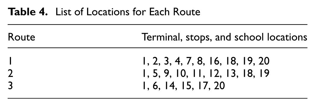
For demonstrating the HAS model, we consider twenty locations including terminal, student stops, and schools on the three routes given in Table 4; location 1 is the bus terminal, 2 to 17 indicate bus stops, and 18 to 20 are schools. Table 5 shows the distance between these locations. For each route, we are to allocate a suitable bus from eighteen available ESBs with different prices and specifications. The bus selected for any route will cover all the locations in that route, and in which pathway they will travel these locations will be determined by the HAS model. Table 6 shows the list and specifications of the buses.

Table 4.

List of Locations for Each Route

Route	Terminal, stops, and school locations
1	1, 2, 3, 4, 7, 8, 16, 18, 19, 20
2	1, 5, 9, 10, 11, 12, 13, 18, 19
3	1, 6, 14, 15, 17, 20

Table 5.

D_lk Matrix

Location no.	1	2	3	4	5	6	7	8	9	10	11	12	13	14	15	16	17	18	19	20
1	na	4.8	3	2.8	1.6	5.9	2.2	2.2	3.3	2.6	6.9	6.6	2.1	2.6	6.7	3.4	2.2	6.3	6.2	4.6
2	4.8	na	0.5	6.5	na	na	2.7	1.9	na	na	na	na	na	na	na	0.8	na	6.2	1.1	5.9
3	3	0.5	na	1.5	na	na	5.1	2.3	na	na	na	na	na	na	na	1.4	na	4.3	6.8	3.8
4	2.8	6.5	1.5	na	na	na	6.8	3.9	na	na	na	na	na	na	na	0.9	na	4	1.3	3.2
5	1.6	na	na	na	na	na	na	na	1.9	4.7	5.4	3.9	5	na	na	na	na	5	6.1	na
6	5.9	na	na	na	na	na	na	na	na	na	na	na	na	6.8	1	na	1.2	na	na	1
7	2.2	2.7	5.1	6.8	na	na	na	0.9	na	na	na	na	na	na	na	4.5	na	5.7	2.4	6.7
8	2.2	1.9	2.3	3.9	na	na	0.9	na	na	na	na	na	na	na	na	5.9	na	6.3	5	2.5
9	3.3	na	na	na	1.9	na	na	na	na	2.4	6.5	4.4	0.7	na	na	na	na	6.4	4.2	na
10	2.6	na	na	na	4.7	na	na	na	2.4	na	1.9	5.8	1.5	na	na	na	na	6.7	0.7	na
11	6.9	na	na	na	5.4	na	na	na	6.5	1.9	na	1.9	6.5	na	na	na	na	3.4	6.8	na
12	6.6	na	na	na	3.9	na	na	na	4.4	5.8	1.9	na	1.2	na	na	na	na	5.7	3.1	na
13	2.1	na	na	na	5	na	na	na	0.7	1.5	6.5	1.2	na	na	na	na	na	6.4	5.2	na
14	2.6	na	0	na	na	6.8	na	na	na	na	na	na	na	na	4.4	na	4.4	na	na	4.6
15	6.7	na	na	na	na	1	na	na	na	na	na	na	na	4.4	na	na	4.4	na	na	5.3
16	3.4	0.8	1.4	0.9	na	0	4.5	5.9	na	na	na	na	na	na	na	na	na	2.2	3.4	3.1
17	2.2	na	na	na	na	1.2	na	na	na	na	na	na	na	4.4	4.4	na	na	na	na	3
18	6.3	6.2	4.3	4	5	na	5.7	6.3	6.4	6.7	3.4	5.7	6.4	na	na	2.2	na	na	0.9	6
19	6.2	1.1	6.8	1.3	6.1	na	2.4	5	4.2	0.7	6.8	3.1	5.2	na	na	3.4	na	0.9	na	2.1
20	4.6	5.9	3.8	3.2	na	1	6.7	2.5	na	na	na	na	na	4.6	5.3	3.1	3	6	2.1	na

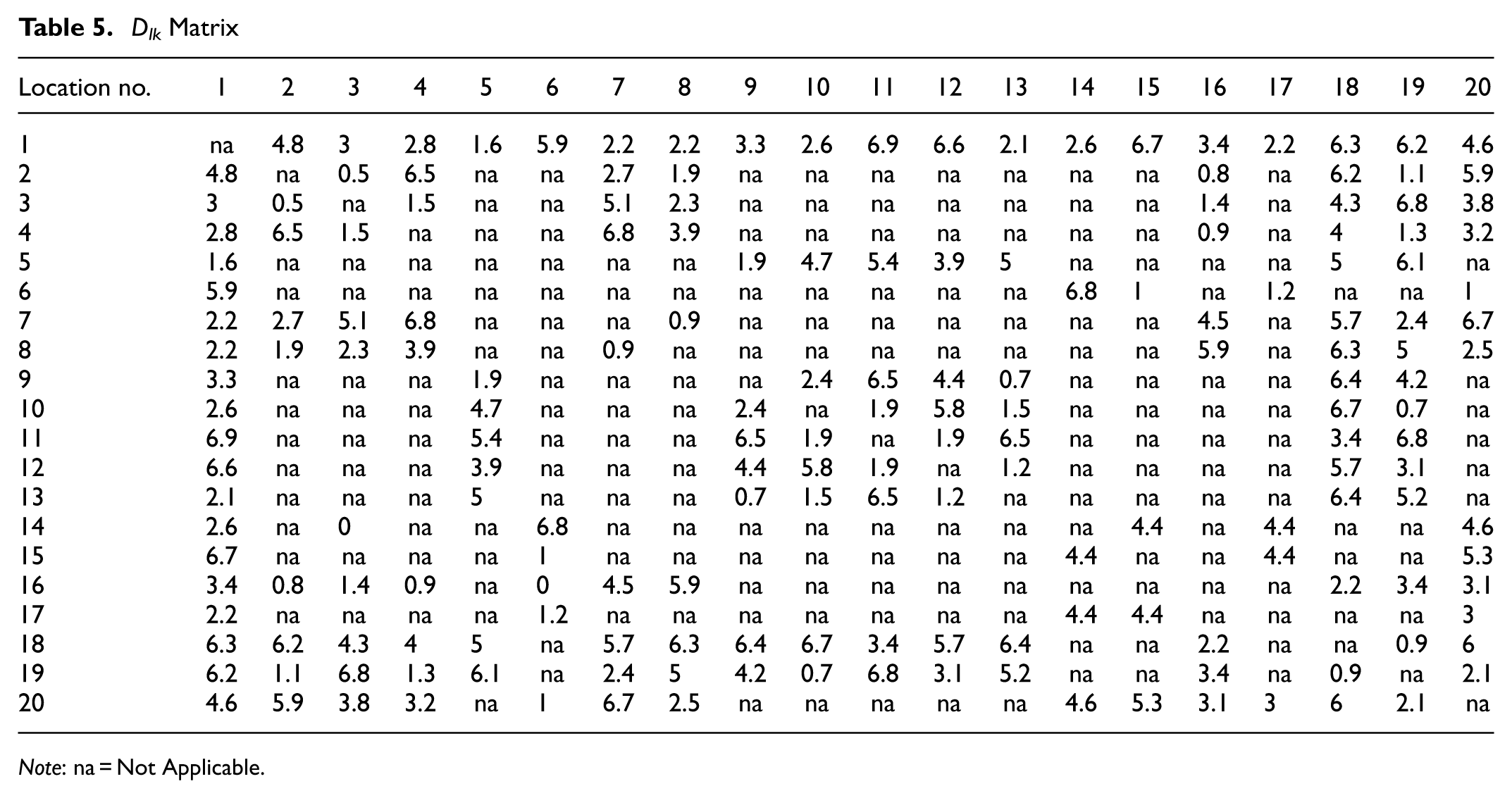
Note: na = Not Applicable.

Table 6.

List of Available Buses and their Specifications

Bus no.	Seating capacity (person)	Battery capacity (kWh)	Bus price (USD)
1	16	68	140,000
2	16	68	140,000
3	24	100	155,000
4	24	100	155,000
5	30	88	160,000
6	30	88	160,000
7	30	88	160,000
8	55	127	210,000
9	55	127	210,000
10	55	127	210,000
11	72	130	270,000
12	72	130	270,000
13	77	155	280,000
14	77	155	280,000
15	84	210	300,000
16	84	210	300,000
17	90	387	350,000
18	90	387	350,000

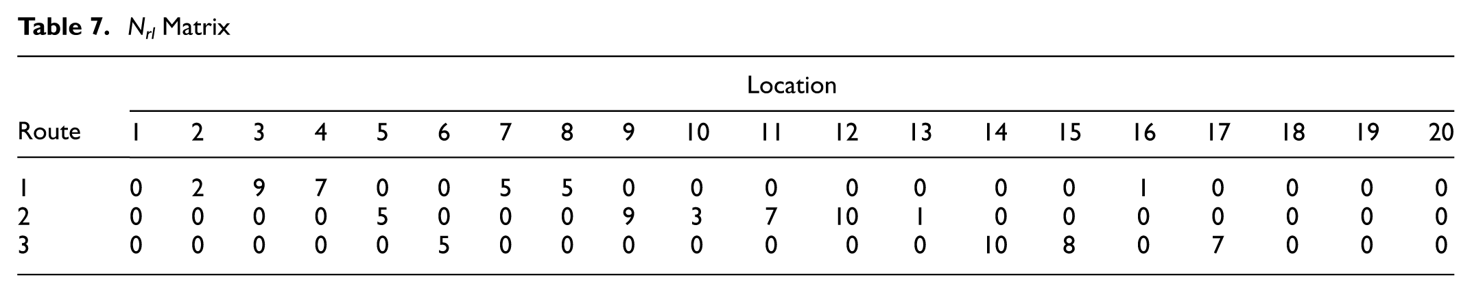
In addition, the N_rl matrix that shows the total number of students to pick from each location in each route is given in Table 7, and the W_rl matrix that indicates which location is included in which route is given in Table 8. In this example, we have also considered the cost of charge consumption C = 1.2 USD/kWh, Time window T_w = 60 min and the battery capacity of a bus required to travel per mile, E = 0.4 kWh.

Table 7.

N_rl Matrix

Route	Location
Route	1	2	3	4	5	6	7	8	9	10	11	12	13	14	15	16	17	18	19	20
1	0	2	9	7	0	0	5	5	0	0	0	0	0	0	0	1	0	0	0	0
2	0	0	0	0	5	0	0	0	9	3	7	10	1	0	0	0	0	0	0	0
3	0	0	0	0	0	5	0	0	0	0	0	0	0	10	8	0	7	0	0	0

Table 8.

W_rl Matrix

Route	Location
Route	1	2	3	4	5	6	7	8	9	10	11	12	13	14	15	16	17	18	19	20
1	1	1	1	1	0	0	1	1	0	0	0	0	0	0	0	1	0	1	1	1
2	1	0	0	0	1	0	0	0	1	1	1	1	1	0	0	0	0	1	1	0
3	1	0	0	0	0	1	0	0	0	0	0	0	0	1	1	0	1	0	0	1

These inputs have been used to solve the model using GAMS software with CPLEX solver. The results of the model are displayed in Table 9. The solution reveals that a total of three buses have been assigned to three routes. Let’s take Route 1 as an example: Bus No. 5 is assigned to this route, beginning at Terminal 1, picking up students at locations 7, 8, 4, 16, 3, and 2 the bus will then drop off the students at School 19, 20, and 18, respectively. After dropping off students, the bus will return to Terminal 1. The results in the table only display the one-way direction because the bus will follow the same path in the opposite direction while returning. This means that the bus will travel from Terminal 1 to School 18, 20, and then to School 19, pick up the students, and drop them off at their respective bus stops at 2, 3, 16, 4, 8, and 7 before returning to Terminal 1. Therefore, as the distance traveled in both directions is the same, we multiplied the total distance by 2 in the objective function. In addition, the main goal of this optimization model is to minimize the total cost; the minimum cost for this example is USD 55,498. In addition, to solve the problem this model took only 0.171 s of CPU time.

Table 9.

Result of the Example from Hybrid Allocation and Sequencing Model

Route	Allocated bus no.	Locations traveled by bus	The sequence of one-way travel
1	5	1, 2, 3, 4, 7, 8, 16, 18, 19, 20	1–7–8–4–16–3–2–19–20–18–1
2	8	1, 5, 9, 10, 11, 12, 13, 18, 19	1–13–10–9–5–12–11–18–19–1
3	6	1, 6, 14, 15, 17, 20	1–14–15–6–17–20–1

Computational Experiments and Results of HAS Model

Just like the MIP-AS optimization model, we utilized GAMS software and the CPLEX solver to solve the HAS model. We analyzed the HAS model’s results for the same eight cases, number of locations, and routes as used in the MIP-AS model, and then expanded the number of cases up to nineteen for larger numbers of locations and routes. The comparison between the first eight cases of the HAS model and the MIP-AS model can be found in Table 10. In addition, Table 11 presents the complete results of the HAS model, including larger problems. It is clear from Table 10 that the HAS model solves significantly faster than the MIP-AS model while maintaining the same level of accuracy, as the objective value (total cost) is nearly identical in both models for each case. In the HAS model, the integration of the heuristic and optimization process significantly reduces the number of variables and constraints, which in turn allows the model to solve the problem much more quickly while using much less memory capacity. For instance, comparing case number 7 for both models, we see that for seventy locations and eight routes, the MIP-AS model has 706,235 variables, whereas the HAS model has only 4,962 variables. Consequently, the HAS model solves the case in just 1.219 s, whereas the MIP-AS model takes almost 54,000 times longer, at 65,874 s, to solve the same case problem. However, the total cost is nearly the same in both models and for this case: 160,538 in the MIP-AS model and 160,793 in the HAS model.

Table 10.

Comparison Between Mixed Integer Programming Allocation Sequencing and Hybrid Allocation and Sequencing Model

Input			Output
				Total costs (USD)		No. of variables		No. of constraints		CPU time (s)		Memory usage (MB)
Case no	No. of locations	No. of routes	No. of allocated bus	MIP-AS	HAS	MIP-AS	HAS	MIP-AS	HAS	MIP-AS	HAS	MIP-AS	HAS
1	10	1	1	19,930	20,008	1,844	110	253	196	0.267	0.18	5	4
2	20	3	3	55,472	55,498	21,721	419	924	744	1.33	0.33	15	4
3	30	3	3	67,434	67,715	48,751	929	1,894	1,704	9.91	0.33	28	5
4	40	4	4	87,532	87,561	115,290	1,636	3,174	2,860	6,182.01	0.59	61	5
5	50	6	6	122,200	122,201	270,385	2,546	5,178	4,560	7,819.14	0.41	135	6
6	60	5	5	113,918	113,990	324,354	3,652	6,783	6,256	31,938.29	0.70	162	7
7	70	8	8	160,538	160,793	706,235	4,962	9,784	9,784	65,874.83	1.22	350	8
8	100	8	8	NA	196,191	1,800,198	10,092	19,383	18,336	>589,000	2.16	>2,570	13

Note: NA = Not Available.

Table 11.

Results for Hybrid Allocation and Sequencing Model

Input			Output
Cases	No. of locations	No. of routes	No. of allocated bus	Total costs (USD)	No. of variables	No. of constraints	CPU time (s)	Memory usage (MB)
1	10	1	1	20,008	110	196	0.188	4
2	20	3	3	55,472	419	744	0.33	4
3	30	3	3	67,434	929	1,704	0.33	5
4	40	4	4	87,532	1,636	2,860	0.59	5
5	50	6	6	122,200	2,546	4,560	0.41	6
6	60	5	5	113,990	3,652	6,256	0.70	7
7	70	8	8	160,793	4,962	9,784	1.22	8
8	80	9	9	188,949	6,476	12,060	2.06	10
9	90	10	10	221,126	8,186	15,360	2.20	12
10	100	8	8	196,191	10,092	18,336	2.16	13
11	200	20	20	451109	40,187	74,676	7.22	41
12	300	25	25	570, 035	90,282	169,066	20.14	88
13	400	30	30	695,709	160,382	305,266	50.99	154
14	500	35	35	825,817	250,482	481,466	112.71	239
15	600	40	40	904,428	360,582	697,666	292.93	343
16	700	40	40	934,483	490,682	953,866	501.53	466
17	800	45	45	1,010,479	640,777	1,242,306	1012.61	606
18	900	45	45	1,053,095	810,877	1,577,506	1714.67	767
19	1000	50	50	1,210,225	1,942,996	1,000,972	2793.22	945

Note: CPU = Central Processing Unit.

To further illustrate this performance gap, Figure 2 provides a side-by-side comparison across the first seven test cases. Panel (a) confirms that the heuristic approach achieves a total cost nearly identical to the exact method. However, panels (b) and (c), plotted on logarithmic scales, visually demonstrate the exponential increase in model complexity (variables) and solution time required by the MIP-AS model, contrasting sharply with the highly scalable performance of the HAS model.

Figure 2.

Result comparison between MIP-AS and HAS model across test cases 1-7, illustrating: (a) total cost, (b) number of variables, and (c) CPU time. Note that panels (b) and (C) are plotted on a logarithmic scale.

Based on the findings from Table 11, the HAS model is fast and efficient at solving large-scale problems. The study tested the model for up to 1,000 locations and fifty routes, and it consistently produced results in a significantly short time while using minimum resources. For example, when solving case no. 19, which had 1,000 locations and fifty routes, the HAS model took only 2,793 s, which is 210 times faster than the time taken by the MIP-AS model to solve a problem with only 100 locations.

Sensitivity Analysis

We carried out a sensitivity analysis to assess the robustness and flexibility of our proposed models. In our sensitivity analysis, we selected case no. 14, which encompasses 500 locations and thirty-five routes. We adjusted key parameters such as bus battery capacity, seating capacity, bus price, charging cost per kWh, battery capacity needed per mile, and number of students at each bus stop to understand how changes in these parameters affect the model’s performance and decision-making results.

The experimental strategy used in this analysis involved changing one factor at a time. This means keeping the initial configuration of each parameter and then gradually changing the value of each parameter by a certain percentage while keeping the other parameters constant. The results of the sensitivity analysis for each run are categorized and reported in Table 12. The results presented in Table 12 show that any changes in the per unit charging cost (C) and the battery capacity required to travel per mile (E) directly affect the total charge consumption cost. However, they don’t have much impact on the bus allocation decision. This means that the total cost changes with the increase or decrease of these parameters, but the allocated buses remain unchanged. Similarly, when the bus price (P_b) increases, the total cost also increases, and when the bus price decreases, the total cost also decreases. In our sensitivity analysis, we increased and decreased the prices of all buses at the same time, and therefore it had no impact on bus allocation decisions. It is evident from the sensitivity analysis that an increase in the battery capacity of the buses results in decreased charge consumption cost and, in turn, total cost. However, a decrease in the battery capacity did not affect the total cost. Nevertheless, with an 85% decrease in battery capacity, the cost increases, and the bus allocation decision changes. The battery capacity has a low impact on cost and bus allocation decisions when the model considers only one complete trip per bus in every school day. Nonetheless, for multiple bus trips per day, battery capacity could have a much greater impact.

Table 12.

Sensitivity Analysis Result-1

Parameter	Percent change	Total charge consumption cost (USD)	Bus procurement cost (USD)	Total cost (USD)	CPU time(s)	Memory usage (MB)
Per unit charging cost, C	+50%	200,727	692,000	892,727	111.83	239
	+25%	167,272	692,000	859,272	109.42	239
	0	133,818	692,000	825,818	112.71	239
	−25%	100,363	692,000	792,363	112.45	239
	−50%	66,909	692,000	758,909	112.08	239
Battery capacity required to travel per mile, E	+50%	200,727	692,000	892,727	109.17	239
	+25%	167,272	692,000	859,272	111.51	239
	0%	133,818	692,000	825,818	112.71	239
	−25%	100,363	692,000	792,363	110.59	239
	−50%	66,909	692,000	758,909	111.19	239
Price of bus, P_b	+50%	133,818	1,033,800	1,167,618	112.36	239
	+25%	133,818	865,000	998,818	112.22	239
	0%	133,818	692,000	825,818	112.71	239
	−25%	133,818	519,000	652,818	110.98	239
	−50%	133,818	346,000	479,818	111.68	239
Battery capacity of bus, F_b	+50%	133,818	692,000	825,818	112.20	239
	+25%	133,818	692,000	825,818	110.87	239
	0%	133,818	692,000	825,818	112.71	239
	−25%	133,818	692,000	825,818	111.65	239
	−50%	133,818	692,000	825,818	111.50	239
	−75%	133,818	692,000	825,818	111.70	239
	−85%	133,818	727,200	861,018	112.41	239
Seating capacity of bus, S_b	+30%	133,818	652,000	785,818	111.72	239
	+20%	133,818	676,800	810,618	112.43	239
	+10%	133,818	688,000	821,818	113.70	239
	0%	133,818	692,000	825,818	112.71	239
	−10%	infeasible	NA	NA	NA	NA
Number of students in each location, N_rl	+10%	infeasible	NA	NA	NA	NA
	0%	133,818	692,000	825,818	112.71	239
	−10%	113,818	688,000	821,818	114.77	239
	−20%	113,818	663,200	797,018	111.13	239
	−30%	113,818	638,400	772,218	113.59	239

Note: CPU = Central Processing Unit; NA = Not Available.

With regard to seating capacity, an increase in seating capacity results in a decrease in total cost as a result of the increased seating capacity, allowing low-priced buses, which were previously not selected because of a shortage of seating capacity, to be selected. Similarly, a decrease in the number of students at each bus stop results in a decrease in the total cost. However, a decrease in seating capacity and an increase in the number of students at each location from the original model led to an infeasible solution. This occurred because route no. 18, consisting of sixteen bus stops, has a total of eighty-eight students, and the maximum seating capacity among the listed buses is ninety seats. Therefore, decreasing the seating capacity of all buses or increasing the number of students at each location meant that the model could not allocate any bus to route 18, as this model considers a single bus for each route. It would not have resulted in an infeasible solution if multiple buses could be used on that route. To check the effect of seating capacity and the number of students at each location on the bus allocation decision, we ran case 14 by decreasing the number of students from all routes and considered it the base model. After that, we checked the impact of those two parameters by increasing and decreasing the seating capacity of buses and the number of students at each location respectively. The results of the analysis are in Table 13.

Table 13.

Sensitivity Analysis Result–2

Parameter name	Percent change	Total charge consumption cost (USD)	Bus procurement cost (USD)	Total cost (USD)	CPU time (s)	Memory usage (MB)
Seating capacity of bus, S_b	+30%	127,171	588,000	715,171	111.75	239
	+20%	127,171	632,400	759,571	112.15	239
	+10%	127,171	654,400	781,571	110.23	239
	0%	127,171	676,800	803,971	114.08	239
	−10%	127,171	688,000	815,171	112.45	239
	−20%	127,171	693,200	820,371	115.28	239
Number of students in each location, N_rl	+30%	127,171	706,000	833,171	112.83	239
	+20%	127,171	692,400	819,571	113.11	239
	+10%	127,171	688,000	815,171	113.33	239
	0%	127,171	676,800	803,971	114.08	239
	−10%	127,171	665,600	792,771	114.46	239
	−20%	127,171	596,000	723,171	109.89	239
	−30%	127,171	560,400	687571	111.04	239

Note: CPU = Central Processing Unit.

Table 13 shows that as the seating capacity of buses increases, the total cost decreases, and when the seating capacity decreases, the total cost increases. This is because of the change in the allocated buses for each increment and decrement. Similarly, as the number of students in each location increases, the total cost decreases, and when the number of students decreases, the total cost increases, reflecting the change in allocated buses.

The sensitivity analysis shows that the total CPU time and memory usage remain consistent regardless of changes in all parameters. Therefore, the CPU time and memory usage depend on the scale of the model, and these parameters do not affect either the CPU time or memory usage. Additionally, as this model permits only a single bus for each route, the number of buses will remain constant, that is thirty-five, regardless of changes in all parameters. However, different buses may be allocated.

Finally, to address potential correlations between strategic parameters, we expanded our analysis to examine the simultaneous interaction between Bus Price (P_b) and Battery Capacity (F_b). This multi-parameter analysis allows us to determine if the impact of bus price changes varies depending on the available battery capacity.

Figure 3 presents a heatmap of the Total Cost under varying combinations of these two factors. The visualization reveals a distinct vertical stratification of color bands. This pattern indicates that whereas the Total Cost changes significantly as we move horizontally (changing Bus Price), it remains largely stable as we move vertically (changing Battery Capacity). This stability suggests that for the studied scenarios, the procurement cost is the dominant driver of the objective function. Even when battery capacity is reduced by 50%, the model does not require shifting to a significantly different fleet composition to satisfy the range constraints.

Figure 3.

Two-parameter sensitivity heatmap illustrates the interaction between bus price ( $P_{b}$ ) and battery capacity ( $F_{b}$ ) on total cost.

To further quantify this behavior, Figure 4 compares the individual sensitivity of Bus Price (Figure 4a) against a multi-factor scenario where Battery Capacity is also varied by ± 50% (Figure 4b). As illustrated in Figure 4b, the cost curves for the varying battery capacity scenarios overlap almost perfectly. This visual convergence demonstrates that the interaction effect of Battery Capacity (F_b) is negligible; reducing capacity by 50% yields virtually the same total cost trajectory as increasing it by 50%. This confirms that fleet procurement decisions in this context are primarily price-sensitive rather than capacity-constrained, validating the robustness of the strategic model against technological variations in battery range.

Figure 4.

Sensitivity of total cost to (a) individual changes in bus price ( $P_{b}$ ) and (b) simultaneous changes in both bus price and battery capacity ( $F_{b}$ ).

To rigorously evaluate the model’s boundary conditions and address the fleet’s operational constraints, we conducted two additional multi-parameter sensitivity analyses. These analyses evaluate the simultaneous interaction of Seating Capacity ( $S_{b}$ ) against Student Demand ( $N_{rl}$ ) and Bus Price ( $P_{b}$ ). The results are visualized as heatmaps in Figure 5.

Figure 5.

Multi-parameter sensitivity heatmaps illustrate the effect of bus seating capacity ( $S_{b}$ ) variations against (a) student demand ( $N_{rl}$ ) and (b) bus price ( $P_{b}$ ). Gray cells indicate infeasible scenarios.

Figure 5a maps Seating Capacity ( $S_{b}$ ) against Student Demand ( $N_{rl}$ ). This analysis is critical for identifying the operational feasibility frontier of the single-bus-per-route assumption. As observed in the matrix, a clear diagonal boundary exists. When student demand increases concurrently with a decrease in seating capacity, the model rapidly reaches an infeasible state (indicated by the gray areas), as no single bus in the available fleet catalog can accommodate the inflated route demand. Conversely, increasing seating capacity widens the feasible region, ensuring route viability even during significant enrollment spikes (up to a 20% increase) and allowing the solver to find cost-effective allocations.

Figure 5b maps Seating Capacity ( $S_{b}$ ) against Bus Price ( $P_{b}$ ). This demonstrates the cost elasticity of capacity upgrades. The vertical variations reaffirm our earlier finding that procurement price ( $P_{b}$ ) remains the overwhelming driver of total cost. However, the matrix also reveals that altering seating capacity forces the model to select different vehicle classes from the available heterogeneous fleet, resulting in minor step-changes in the total optimized cost. Notably, severe reductions in seating capacity (−10% and −20%) trigger infeasibilities at baseline prices, though shifting market prices can occasionally open alternative allocation pathways. Together, these combined analyses confirm that whereas financial performance is heavily price sensitive, operational feasibility is strictly bounded by the $S_{b} \times N_{rl}$ interaction.

In summary, the comprehensive sensitivity analysis identifies distinct drivers for operational feasibility versus financial performance. Whereas seating capacity and student demand are the primary determinants of fleet allocation (determining which buses are required), bus procurement price emerges as the dominant driver of total project cost. Interestingly, battery capacity demonstrated high robustness, having minimal impact on cost or allocation within the studied range for single-trip schedules. These findings suggest that strategic planners should prioritize accurate ridership forecasting and capital cost negotiation, in relation to battery range as a secondary constraint for standard, single-route operations, though its importance would likely increase in multi-trip scenarios.

Conclusions

The paper outlined the development of effective and efficient mathematical modeling for assigning ESBs to established routes and identifying the most cost-effective travel sequence along each route. The allocation of buses and the determination of travel sequences are vital for school authorities planning to switch from conventional school buses powered by internal combustion engines to ESBs, considering student health and government initiatives, while keeping the current routes unchanged. To serve this purpose, the paper addressed two solving approaches: the MIP-AS optimization model and the HAS model. In computational cases encompassing varying parameters the effectiveness of both models became apparent as regards computing total cost. The MIP-AS model maintained its accuracy in small computational cases with up to seventy locations but struggled beyond this point, unable to provide results within reasonable timeframes, thus revealing its constraints in handling larger-scale problems. On the other hand, the HAS model consistently delivered precise and swift solutions in nineteen computational cases, even up to 1,000 locations, demonstrating its robustness. Although both models are accurate, the HAS model is notably quicker. The HAS model is highly scalable, requiring minimal computational time and hardware, making it useful for situations that demand quick, accurate decision-making.

This HAS approach model with its hybrid nature not only facilitates the optimization of ESB allocation and travel sequencing for existing routes but also exhibits promise for addressing larger, NP-hard problems where traditional optimization models may prove inadequate. Future research should extend this work to build more comprehensive models. Key extensions include incorporating school bell times to allow for a single bus to serve multiple routes, integrating intermediate charging schedules and locations, and accounting for dynamic variables like traffic conditions and student waiting times. Furthermore, including driver availability and associated personnel costs would enhance the model’s practical utility. This broader scope would offer a more comprehensive solution to ESB scheduling, ensuring that buses are not only optimally allocated but also efficiently utilized throughout their operational periods.

Limitations

It is important to recognize the limitations of this study. The computational experiments relied on synthetically generated datasets. This approach effectively tested the scalability of the algorithms across different problem sizes, but the model has not yet been validated with real-world operational data. As a result, we did not empirically test factors like local topography, traffic patterns, and seasonal temperature variations that directly affect battery performance. Future research should apply the HAS model to real-world case studies to confirm its operational reliability alongside its theoretical scalability.

Footnotes

Author Contributions

The authors confirm contribution to the paper as follows: study conception and design: R. Saha, M. S. Osman; data collection: R. Saha; analysis and interpretation of results: R. Saha; draft manuscript preparation: R. Saha. All authors reviewed the results and approved the final version of the manuscript.

Declaration of Conflicting Interests

The authors declared no potential conflicts of interest with respect to the research, authorship, and/or publication of this article.

Funding

The authors received no financial support for the research, authorship, and/or publication of this article.

ORCID iDs

Rajesh Saha

Mojahid Saeed Osman

References

EPA. Inventory of U.S. Greenhouse Gas Emissions and Sinks: 1990-2022. Report No. EPA 430R-24004. U.S. Environmental Protection Agency, 2024. https://www.epa.gov/ghgemissions/inventory-us-greenhouse-gas-emissions-and-sinks-1990-2022.

Hulagu

Celikoglu

H. B.

Environment-Friendly School Bus Routing Problem with Heterogeneous Fleet: A Large-Scale Real Case. IEEE Transactions on Intelligent Transportation Systems, Vol. 23, No. 4, 2020, pp. 3461–3471. https://doi.org/10.1109/TITS.2020.3036696.

Austin

Heutel

Kreisman

School Bus Emissions, Student Health and Academic Performance. Economics of Education Review, Vol. 70, 2019, pp. 109–126. https://doi.org/10.1016/j.econedurev.2019.03.002.

Lazer

Freehafer

Zepka

A Dataset of Electric School Bus Adoption in the United States. World Resources Institute, 2024. https://doi.org/10.46830/writn.21.00134.v8.

Saha

Osman

M. S.

Computational Model for Re-Routing and Assigning ESBs. Proc., 9th North American Conference on Industrial Engineering and Operations Management, Washington, D.C., June 4–6, 2024.

Ellegood

W. A.

Solomon

North

Campbell

J. F.

School Bus Routing Problem: Contemporary Trends and Research Directions. Omega, Vol. 95, 2020, p. 102056. https://doi.org/10.1016/j.omega.2019.03.014.

Sarubbi

J. F.

Mesquita

C. M.

Wanner

E. F.

Santos

V. F.

Silva

C. M.

A Strategy for Clustering Students Minimizing the Number of Bus Stops for Solving the School Bus Routing Problem. Proc., NOMS 2016-2016 IEEE/IFIP Network Operations and Management Symposium, Istanbul, Turkey, IEEE, New York, 2016, pp. 1175–1180.

Riera-Ledesma

Salazar-González

J. J.

A Column Generation Approach for a School Bus Routing Problem with Resource Constraints. Computers & Operations Research, Vol. 40, No. 2, 2013, pp. 566–583. https://doi.org/10.1016/j.cor.2012.08.011.

Schittekat

Kinable

Sörensen

Sevaux

Spieksma

Springael

A Metaheuristic for the School Bus Routing Problem with Bus Stop Selection. European Journal of Operational Research, Vol. 229, No. 2, 2013, pp. 518–528. https://doi.org/10.1016/j.ejor.2013.02.025.

10.

Calvete

H. I.

Galé

Iranzo

J. A.

Toth

A Partial Allocation Local Search Matheuristic for Solving the School Bus Routing Problem with Bus Stop Selection. Mathematics, Vol. 8, No. 8, 2020, p. 1214. https://doi.org/10.3390/math8081214.

11.

Sciortino

Lewis

Thompson

A school Bus Routing Heuristic Algorithm Allowing Heterogeneous Fleets and Bus Stop Selection. SN Computer Science, Vol. 4, No. 1, 2022, p. 74. https://doi.org/10.1007/s42979-022-01466-6.

12.

Ellegood

W. A.

Campbell

J. F.

North

Continuous Approximation Models for Mixed Load School Bus Routing. Transportation Research Part B: Methodological, Vol. 77, 2015, pp. 182–198. https://doi.org/10.1016/j.trb.2015.03.018.

13.

Yao

Cao

Wang

Zhang

A Two-Stage Heuristic Algorithm for the School Bus Routing Problem with Mixed Load Plan. Transportation Letters, Vol. 8, No. 4, 2016, pp. 205–219. https://doi.org/10.1080/19427867.2015.1110953.

14.

Shang

Yang

Zeng

Tong

L. C.

Solving School Bus Routing Problem with Mixed-Load Allowance for Multiple Schools. Computers & Industrial Engineering, Vol. 151, 2021, p. 106916. https://doi.org/10.1016/j.cie.2020.106916.

15.

Bertsimas

Delarue

Martin

Optimizing schools’ Start Time and Bus Routes. Proceedings of the National Academy of Sciences, Vol. 116, No. 13, 2019, pp. 5943–5948. https://doi.org/10.1073/pnas.1811462116.

16.

Qian

A Neural Combinatorial Approach for School Bus Routing System Optimization. Doctoral dissertation. Northeastern University, Boston, Massachusetts, 2023. https://www.proquest.com/docview/2808521218?pq-origsite=gscholar&fromopenview=true&sourcetype=Dissertations%20&%20Theses.

17.

Orejuela

J. P.

Hernandez

G. J.

Time Dependent School Bus Routing. Revista Espacios, Vol. 40, No. 15, 2019, p. 24. https://www.revistaespacios.com/a19v40n15/19401524.html.

18.

Hou

Y. E.

Dang

L. X.

Kong

Y. F.

Wang

Z. Y.

Zhao

Q. J.

A Hybrid Metaheuristic Algorithm for the Heterogeneous School Bus Routing Problem and a Real Case Study. IAENG International Journal of Computer Science, Vol. 47, No. 4, 2020, pp. 775–785. https://www.iaeng.org/IJCS/current_issue.html.

19.

Ansari

Farrokhvar

Kamali

Integrated Student to School Assignment and School Bus Routing Problem for Special Needs Students. Transportation Research Part E: Logistics and Transportation Review, Vol. 152, 2021, p. 102416. https://doi.org/10.1016/j.tre.2021.102416.

20.

Shafahi

Aliari

Haghani

Balanced Scheduling of School Bus Trips using a Perfect Matching Heuristic. Transportation Research Record: Journal of the Transportation Research Board, 2018. 2672: 1–11.

21.

Chow

J. Y. J.

School Bus Routing Problem with a Mixed Ride, Mixed Load, and Heterogeneous Fleet. Transportation Research Record: Journal of the Transportation Research Board, 2021. 2675: 467–479.

22.

Taş

Electric Vehicle Routing with Flexible Time Windows: A Column Generation Solution Approach. Transportation Letters, Vol. 13, No. 2, 2021, pp. 97–103. https://doi.org/10.1080/19427867.2020.1711581.

23.

Chen

Hao

J. K.

The Time-Dependent Electric Vehicle Routing Problem: Model and solution. Expert Systems with Applications, Vol. 161, 2020, p. 113593. https://doi.org/10.1016/j.eswa.2020.113593.

24.

Basso

Kulcsár

Sanchez-Diaz

Dynamic Stochastic Electric Vehicle Routing with Safe Reinforcement Learning. Transportation Research Part E: Logistics and Transportation Review, Vol. 157, 2022, p. 102496. https://doi.org/10.1016/j.tre.2021.102496.

25.

Zhang

Zheng

Abdullah

M. G.

Dong

Mixed Electric Bus Fleet Scheduling Problem with Partial Mixed-Route and Partial Recharging. International Journal of Sustainable Transportation, Vol. 16, No. 1, 2022, pp. 73–83. https://doi.org/10.1080/15568318.2021.1914791.

26.

Hiermann

Puchinger

Ropke

Hartl

R. F.

The Electric Fleet Size and Mix Vehicle Routing Problem with Time Windows and Recharging Stations. European Journal of Operational Research, Vol. 252, No. 3, 2016, pp. 995–1018. https://doi.org/10.1016/j.ejor.2016.01.038.

27.

Rogge

Van der Hurk

Larsen

Sauer

D. U.

Electric Bus Fleet Size and Mix Problem with Optimization of Charging Infrastructure. Applied Energy, Vol. 211, 2018, pp. 282–295. https://doi.org/10.1016/j.apenergy.2017.11.051.

28.

Yıldırım

Ş.

Yıldız

Electric Bus Fleet Composition and Scheduling. Transportation Research Part C: Emerging Technologies, Vol. 129, 2021, p. 103197. https://doi.org/10.1016/j.trc.2021.103197.

29.

Perumal

S. S.

Lusby

R. M.

Larsen

Electric Bus Planning & Scheduling: A Review of Related Problems and Methodologies. European Journal of Operational Research, Vol. 301, No. 2, 2022, pp. 395–413. https://doi.org/10.1016/j.ejor.2021.10.058.

Location no.	1	2	3	4	5	6	7	8	9	10	11	12	13	14	15	16	17	18	19	20
1	na	4.8	3	2.8	1.6	5.9	2.2	2.2	3.3	2.6	6.9	6.6	2.1	2.6	6.7	3.4	2.2	6.3	6.2	4.6
2	4.8	na	0.5	6.5	na	na	2.7	1.9	na	na	na	na	na	na	na	0.8	na	6.2	1.1	5.9
3	3	0.5	na	1.5	na	na	5.1	2.3	na	na	na	na	na	na	na	1.4	na	4.3	6.8	3.8
4	2.8	6.5	1.5	na	na	na	6.8	3.9	na	na	na	na	na	na	na	0.9	na	4	1.3	3.2
5	1.6	na	na	na	na	na	na	na	1.9	4.7	5.4	3.9	5	na	na	na	na	5	6.1	na
6	5.9	na	na	na	na	na	na	na	na	na	na	na	na	6.8	1	na	1.2	na	na	1
7	2.2	2.7	5.1	6.8	na	na	na	0.9	na	na	na	na	na	na	na	4.5	na	5.7	2.4	6.7
8	2.2	1.9	2.3	3.9	na	na	0.9	na	na	na	na	na	na	na	na	5.9	na	6.3	5	2.5
9	3.3	na	na	na	1.9	na	na	na	na	2.4	6.5	4.4	0.7	na	na	na	na	6.4	4.2	na
10	2.6	na	na	na	4.7	na	na	na	2.4	na	1.9	5.8	1.5	na	na	na	na	6.7	0.7	na
11	6.9	na	na	na	5.4	na	na	na	6.5	1.9	na	1.9	6.5	na	na	na	na	3.4	6.8	na
12	6.6	na	na	na	3.9	na	na	na	4.4	5.8	1.9	na	1.2	na	na	na	na	5.7	3.1	na
13	2.1	na	na	na	5	na	na	na	0.7	1.5	6.5	1.2	na	na	na	na	na	6.4	5.2	na
14	2.6	na	0	na	na	6.8	na	na	na	na	na	na	na	na	4.4	na	4.4	na	na	4.6
15	6.7	na	na	na	na	1	na	na	na	na	na	na	na	4.4	na	na	4.4	na	na	5.3
16	3.4	0.8	1.4	0.9	na	0	4.5	5.9	na	na	na	na	na	na	na	na	na	2.2	3.4	3.1
17	2.2	na	na	na	na	1.2	na	na	na	na	na	na	na	4.4	4.4	na	na	na	na	3
18	6.3	6.2	4.3	4	5	na	5.7	6.3	6.4	6.7	3.4	5.7	6.4	na	na	2.2	na	na	0.9	6
19	6.2	1.1	6.8	1.3	6.1	na	2.4	5	4.2	0.7	6.8	3.1	5.2	na	na	3.4	na	0.9	na	2.1
20	4.6	5.9	3.8	3.2	na	1	6.7	2.5	na	na	na	na	na	4.6	5.3	3.1	3	6	2.1	na

Location no.	1	2	3	4	5	6	7	8	9	10	11	12	13	14	15	16	17	18	19	20
1	na	4.8	3	2.8	1.6	5.9	2.2	2.2	3.3	2.6	6.9	6.6	2.1	2.6	6.7	3.4	2.2	6.3	6.2	4.6
2	4.8	na	0.5	6.5	na	na	2.7	1.9	na	na	na	na	na	na	na	0.8	na	6.2	1.1	5.9
3	3	0.5	na	1.5	na	na	5.1	2.3	na	na	na	na	na	na	na	1.4	na	4.3	6.8	3.8
4	2.8	6.5	1.5	na	na	na	6.8	3.9	na	na	na	na	na	na	na	0.9	na	4	1.3	3.2
5	1.6	na	na	na	na	na	na	na	1.9	4.7	5.4	3.9	5	na	na	na	na	5	6.1	na
6	5.9	na	na	na	na	na	na	na	na	na	na	na	na	6.8	1	na	1.2	na	na	1
7	2.2	2.7	5.1	6.8	na	na	na	0.9	na	na	na	na	na	na	na	4.5	na	5.7	2.4	6.7
8	2.2	1.9	2.3	3.9	na	na	0.9	na	na	na	na	na	na	na	na	5.9	na	6.3	5	2.5
9	3.3	na	na	na	1.9	na	na	na	na	2.4	6.5	4.4	0.7	na	na	na	na	6.4	4.2	na
10	2.6	na	na	na	4.7	na	na	na	2.4	na	1.9	5.8	1.5	na	na	na	na	6.7	0.7	na
11	6.9	na	na	na	5.4	na	na	na	6.5	1.9	na	1.9	6.5	na	na	na	na	3.4	6.8	na
12	6.6	na	na	na	3.9	na	na	na	4.4	5.8	1.9	na	1.2	na	na	na	na	5.7	3.1	na
13	2.1	na	na	na	5	na	na	na	0.7	1.5	6.5	1.2	na	na	na	na	na	6.4	5.2	na
14	2.6	na	0	na	na	6.8	na	na	na	na	na	na	na	na	4.4	na	4.4	na	na	4.6
15	6.7	na	na	na	na	1	na	na	na	na	na	na	na	4.4	na	na	4.4	na	na	5.3
16	3.4	0.8	1.4	0.9	na	0	4.5	5.9	na	na	na	na	na	na	na	na	na	2.2	3.4	3.1
17	2.2	na	na	na	na	1.2	na	na	na	na	na	na	na	4.4	4.4	na	na	na	na	3
18	6.3	6.2	4.3	4	5	na	5.7	6.3	6.4	6.7	3.4	5.7	6.4	na	na	2.2	na	na	0.9	6
19	6.2	1.1	6.8	1.3	6.1	na	2.4	5	4.2	0.7	6.8	3.1	5.2	na	na	3.4	na	0.9	na	2.1
20	4.6	5.9	3.8	3.2	na	1	6.7	2.5	na	na	na	na	na	4.6	5.3	3.1	3	6	2.1	na

Location no.	1	2	3	4	5	6	7	8	9	10	11	12	13	14	15	16	17	18	19	20
1	na	4.8	3	2.8	1.6	5.9	2.2	2.2	3.3	2.6	6.9	6.6	2.1	2.6	6.7	3.4	2.2	6.3	6.2	4.6
2	4.8	na	0.5	6.5	na	na	2.7	1.9	na	na	na	na	na	na	na	0.8	na	6.2	1.1	5.9
3	3	0.5	na	1.5	na	na	5.1	2.3	na	na	na	na	na	na	na	1.4	na	4.3	6.8	3.8
4	2.8	6.5	1.5	na	na	na	6.8	3.9	na	na	na	na	na	na	na	0.9	na	4	1.3	3.2
5	1.6	na	na	na	na	na	na	na	1.9	4.7	5.4	3.9	5	na	na	na	na	5	6.1	na
6	5.9	na	na	na	na	na	na	na	na	na	na	na	na	6.8	1	na	1.2	na	na	1
7	2.2	2.7	5.1	6.8	na	na	na	0.9	na	na	na	na	na	na	na	4.5	na	5.7	2.4	6.7
8	2.2	1.9	2.3	3.9	na	na	0.9	na	na	na	na	na	na	na	na	5.9	na	6.3	5	2.5
9	3.3	na	na	na	1.9	na	na	na	na	2.4	6.5	4.4	0.7	na	na	na	na	6.4	4.2	na
10	2.6	na	na	na	4.7	na	na	na	2.4	na	1.9	5.8	1.5	na	na	na	na	6.7	0.7	na
11	6.9	na	na	na	5.4	na	na	na	6.5	1.9	na	1.9	6.5	na	na	na	na	3.4	6.8	na
12	6.6	na	na	na	3.9	na	na	na	4.4	5.8	1.9	na	1.2	na	na	na	na	5.7	3.1	na
13	2.1	na	na	na	5	na	na	na	0.7	1.5	6.5	1.2	na	na	na	na	na	6.4	5.2	na
14	2.6	na	0	na	na	6.8	na	na	na	na	na	na	na	na	4.4	na	4.4	na	na	4.6
15	6.7	na	na	na	na	1	na	na	na	na	na	na	na	4.4	na	na	4.4	na	na	5.3
16	3.4	0.8	1.4	0.9	na	0	4.5	5.9	na	na	na	na	na	na	na	na	na	2.2	3.4	3.1
17	2.2	na	na	na	na	1.2	na	na	na	na	na	na	na	4.4	4.4	na	na	na	na	3
18	6.3	6.2	4.3	4	5	na	5.7	6.3	6.4	6.7	3.4	5.7	6.4	na	na	2.2	na	na	0.9	6
19	6.2	1.1	6.8	1.3	6.1	na	2.4	5	4.2	0.7	6.8	3.1	5.2	na	na	3.4	na	0.9	na	2.1
20	4.6	5.9	3.8	3.2	na	1	6.7	2.5	na	na	na	na	na	4.6	5.3	3.1	3	6	2.1	na