Sage Journals: Discover world-class research

Abstract

Priced managed lanes (MLs) have been widely implemented in metropolitan areas to provide faster and more reliable travel while generating revenue to fund transportation improvements. Successful implementation of MLs relies on the careful selection of roadways on which to build MLs. This, in turn, relies on accurate travel demand models. Although existing models have been effective in forecasting aggregate travel demand and toll revenues, they often fall short in capturing individual lane decisions. Notably, MLs do not always deliver faster travel compared with adjacent toll-free lanes, called general-purpose lanes. Instances in which MLs have resulted in longer travel times can lead to user distrust and dissatisfaction. Despite this, there is no prior research investigating how negative ML experiences affect future lane choice behavior. Therefore, this study employs a logit regression analysis using 30 months of data from the Katy Freeway, Houston, TX to model individual lane choice decisions and examine the impact of slower ML events on subsequent travel behavior. The results indicated that drivers tend to pay tolls for using MLs when toll rates and speeds are higher. This indicates that travelers are generally willing to pay for faster travel. Conversely, travelers who experienced or observed slower ML events were less likely to use MLs in the future, revealing risk-averse behavior. Although this effect diminished over time as drivers tended to forget the event, repeated exposure to similar incidents reinforced the memory and prolonged the deterrent effect.

Keywords

managed lanes travel behavior travel time differential

Introduction

Managed lanes (MLs) require travelers to meet specific requirements to use the lanes. They usually provide a faster, more reliable trip than the toll-free adjacent lanes, called general-purpose lanes (GPLs). High-occupancy toll (HOT) lanes are the most common form of priced MLs, which allow high-occupancy vehicles (HOVs) to use them for free or at a reduced toll, whereas single-occupancy vehicles (SOVs) have to pay the full toll. Over 80 HOT lane facilities have been implemented in the United States ( 1 ). MLs generally offer faster, safer, and more reliable travel for drivers and generate revenue for agencies to support the operation, maintenance, and potential expansion of transportation infrastructure ( 2 – 4 ).

However, the implementation and success of ML projects hinge on reliable demand forecasting based on a sufficient understanding of travel behavior. Several models use the value of time (VOT)—the amount travelers are willing to pay to save time—and the value of reliability (VOR)—the amount travelers are willing to pay to reduce travel time variability—as key factors in predicting lane choice behavior ( 5 , 6 ). Although these models deliver reasonable demand predictions at an aggregate level, they often struggle to account for individual traveler decisions ( 2 ). The complexity, dynamism, context dependence, and heterogeneity in individual preferences make travel behavior particularly difficult to model and understand. Therefore, a discrete choice model is commonly applied to address this challenge ( 7 ).

In discrete choice analysis, many studies commonly use survey data to model travel behavior on MLs ( 8 , 9 ). Such survey data not only captures travelers’ observed choices under real-world conditions but also investigate traveler responses to potential policies or pricing strategies that do not yet exist. Despite the advantages of the survey, the collection process can be costly and the sample sizes limited. However, advancements in technologies, such as electronic toll collection systems and automatic vehicle identification (AVI) sensors, have facilitated alternative data collection methods that are cost-effective and reflective of actual traveler behavior on MLs. A dataset collected in this manner, including longitudinal observations that capture the travel choices of the same travelers over time, is referred to as panel data. A large-scale panel dataset was collected, encompassing all transponder-recorded trips along the Katy Freeway, Houston, TX from January 2012 to September 2014 ( 2 ). To the best of the authors’ knowledge, no prior studies have applied discrete choice modeling techniques to such long-term panel data. This research is the first to leverage long-horizon data to model lane choice decisions.

In addition to the long-horizon data, empirical data from the I-85 in Atlanta (GA), I-405 in Seattle (WA), North Tarrant Express in Dallas-Fort Worth (TX), and the Katy Freeway in Houston (TX) indicate that using MLs does not always result in faster travel ( 2 , 5 , 10 , 11 ). Travelers generally expect that MLs that require payment for access will offer superior travel times compared with GPLs. When this expectation is not met as a result of unexpected slowdowns in MLs, it raises important questions about how such incidents influence subsequent lane choice behavior. However, to date, no studies have examined the impact of slower ML conditions on future traveler decisions. This study is the first to incorporate the effect of slower ML incidents into a predictive model of lane choice behavior.

Literature Review

Research on MLs has primarily focused on travelers’ willingness to pay tolls in exchange for travel time savings, with models typically emphasizing the trade-off between cost and time. More recently, travel time reliability has also been incorporated, based on the assumption that travelers value a more predictable commute and are willing to pay for it ( 9 , 12 , 13 ). This assumption is supported by survey findings, which indicate that many travelers are indeed willing to pay for both travel time savings and reliability ( 5 , 6 ). Various modeling techniques have been employed to estimate VOT and VOR to forecast ML usage. These models have been reasonably effective in forecasting traffic demand and revenue; however, they fail to capture individual lane-choice decision making ( 2 ).

Numerous studies have explored various methods of modeling individual lane choice. Among these, a logit model with random utility maximization (RUM) has been widely adopted, incorporating socioeconomic and trip characteristics to predict individual lane selection ( 14 , 15 ). However, the logit model assumes homogeneous preferences, which may not accurately reflect the complexity and variability of human behavior. To address this limitation, mixed logit models have been employed to capture unobserved heterogeneity among individuals ( 16 , 17 ). Toledo and Sharif employed a mixed logit to examine the information effect on ML lane choice ( 18 ). When travel time information was not provided, travelers were more inclined to choose MLs. Xie et al. introduced a personalized choice model that integrates personal historical information into a mixed logit model to improve the prediction of ML usage ( 7 ). Their findings indicate that incorporating individual historical factors, such as ML loyalty, speed differences between the current trip and the average of previous trips, and travel time difference between the most recent ML trip and the current anticipated travel time, significantly enhances predictive performance.

In addition to conventional choice modeling approaches that incorporate socioeconomic and trip characteristics, recent studies have applied psychological concepts and behavioral economics to better understand lane choice decisions. Green and Burris used psychological survey questions to investigate how travelers decide between driving alone or carpooling, and between using MLs or GPLs ( 19 ). Their findings suggest that travelers who mostly respect speed limits tend to drive alone on GPLs rather than MLs—most likely because they are satisfied with the slower, but toll-free, speeds on GPLs. Additionally, travelers who are uncomfortable with uncertain situations are less likely to carpool on MLs than to drive alone on GPLs, possibly because they wish to avoid the uncertainty associated with carpooling, such as variability in passenger arrangements or waiting times. Since traditional travel behavior models do not incorporate risk, Huang et al. developed a cumulative prospect theory model that did incorporate risk to predict the use of MLs ( 20 ). Their findings indicate that travelers exhibit greater risk aversion when facing the possibility of being late, compared with the prospect of saving travel time. Additionally, travelers display overly optimistic behavior when there is a higher likelihood of experiencing longer travel times.

Furthermore, the empirical data have revealed the surprising finding that travel speeds on MLs are sometimes slower than GPLs (2). Although prior studies have explored the influence of socioeconomic factors, trip characteristics, and psychological traits on individual lane choice, no study has investigated the impact of experiences with slower MLs. To bridge this gap, this study employed a logistic regression analysis on the Katy Freeway data to model individual lane choice decisions and examine whether experiencing or observing a slower ML event affects future ML usage.

Modeling Lane Choice: Methodology

Katy Freeway

The I-10 Katy Freeway connects the city of Katy to downtown Houston and includes a 12-mi segment with up to six GPLs and two variably priced MLs in each direction, separated by flexible pylons. MLs generally provide shorter travel times and greater travel time reliability than the adjacent GPLs because they typically operate at free-flow or near free-flow speeds, whereas GPLs frequently experience congestion during peak hours (see Figure 1). Both MLs and GPLs have the same posted speed limit. Additionally, travelers on the GPL can directly observe conditions on the MLs. Dynamic message signs along the corridor display travel times for the GPLs, while other signs display the ML toll rates to key destinations ( 2 ). Based on these conditions, it was assumed that travelers had sufficient information to make lane choice decisions if they were interested in choosing between lanes.

Figure 1.

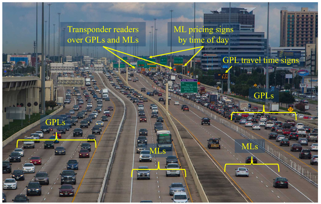
Katy Freeway ( 21 ).

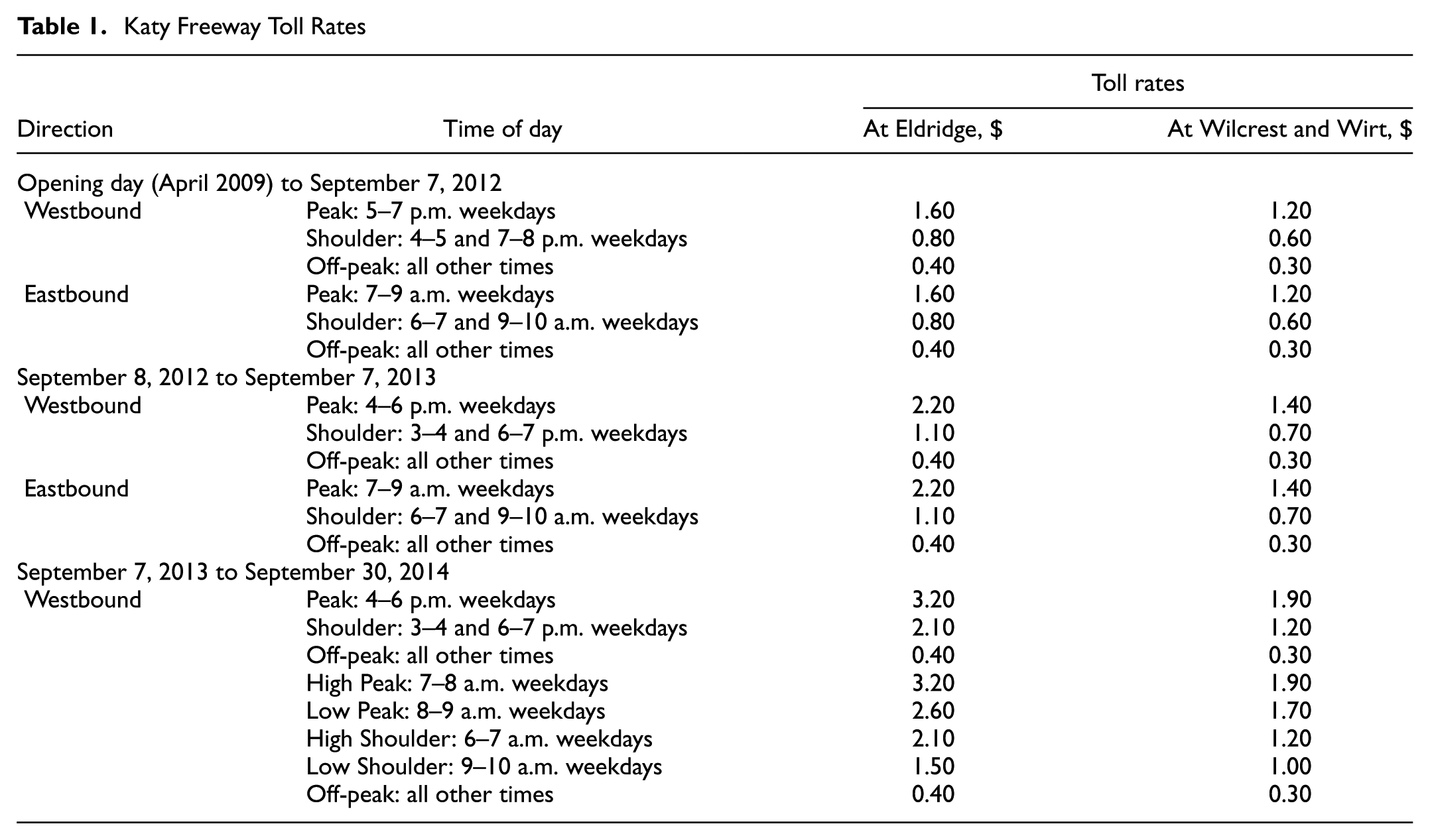
Travelers using the MLs must pay toll rates that vary based on the time of day, referred to as variable tolling, and vehicle occupancy ( 22 ). HOVs with at least two occupants (including the driver) and motorcycles are exempt from toll charges during designated HOV-free periods, which occur on weekdays from 5:00 to 11:00 a.m. and from 2:00 to 8:00 p.m. To qualify for this exemption, travelers must use the leftmost MLs at toll plazas. Outside of these periods, HOVs and motorcycles are subject to the same toll rates as SOVs. Additionally, this facility supports two payment methods: prepaid payment using transponders (toll tags) and postpaid payment based on license plate identification. Owing to an additional processing fee, license plate payments incur a higher toll charge than transponder payments ( 2 ).

Data Collection

The Texas Department of Transportation and Harris County Toll Road Authority operate AVI sensors installed along the MLs and GPLs at many locations (see Figure 2) ( 23 ). These sensors detect vehicles equipped with transponders and record the unique transponder ID, date and time of detection, and toll paid (if on MLs). Each unique transponder ID should relate to a specific vehicle. The vehicle may not always be driven by the same person, but in most cases would have the same driver and we assumed a one-to-one correspondence between transponder ID and traveler. This analysis used data from January 2012 to September 2014. However, data for December 2012 and October 2013 were missing because of collection issues. The dataset excluded ML travelers who were exempt from toll payments, including HOVs during HOV-free periods, buses, and emergency vehicles. This dataset contained more than 100-million trips of ML travelers paying tolls and GPL travelers. Trips were treated as panel data because multiple trips were collected from the same unique transponder ID over time.

Figure 2.

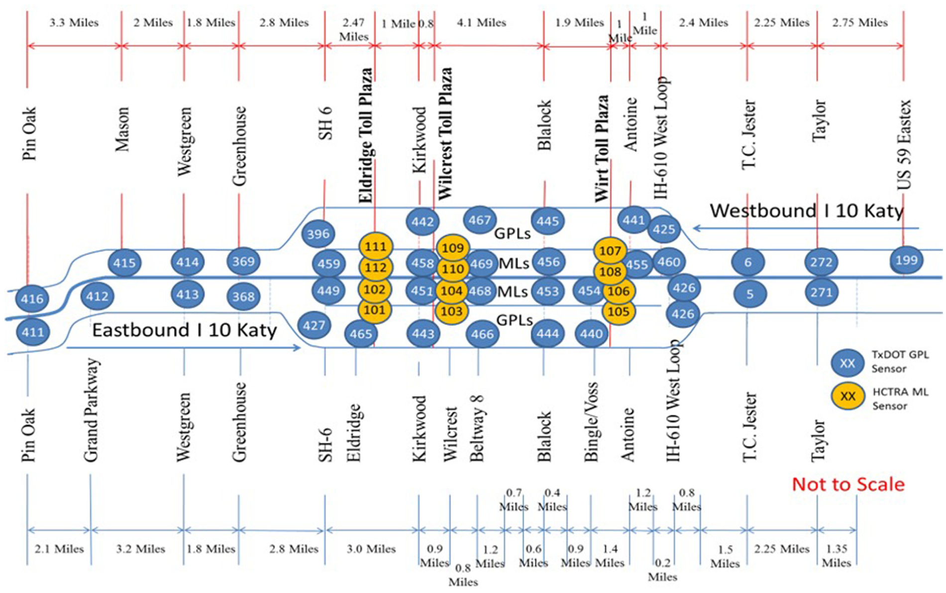
AVI sensors along Katy Freeway.

To protect traveler privacy, each original transponder ID was removed and replaced with a randomly generated unique identifier, ensuring that individual travelers could not be identified from the dataset. However, these anonymized IDs allowed the tracking of trips made by the same traveler over the 31-month study period. Travel time and distance of observed trips were calculated using detection time and location. The average observed speed was then computed using travel time and distance. Because toll prices on the Katy Freeway were set according to variable tolling, the toll rate of each trip was determined using detection time ( 23 ). We identified whether drivers traveled during peak hours or shoulder hours (i.e., transitional periods between peak and off-peak). Peak hours and shoulder hours are defined in Table 1 ( 2 ).

Table 1.

Katy Freeway Toll Rates

		Toll rates
Direction	Time of day	At Eldridge, $	At Wilcrest and Wirt, $
Opening day (April 2009) to September 7, 2012
Westbound	Peak: 5–7 p.m. weekdays	1.60	1.20
	Shoulder: 4–5 and 7–8 p.m. weekdays	0.80	0.60
	Off-peak: all other times	0.40	0.30
Eastbound	Peak: 7–9 a.m. weekdays	1.60	1.20
	Shoulder: 6–7 and 9–10 a.m. weekdays	0.80	0.60
	Off-peak: all other times	0.40	0.30
September 8, 2012 to September 7, 2013
Westbound	Peak: 4–6 p.m. weekdays	2.20	1.40
	Shoulder: 3–4 and 6–7 p.m. weekdays	1.10	0.70
	Off-peak: all other times	0.40	0.30
Eastbound	Peak: 7–9 a.m. weekdays	2.20	1.40
	Shoulder: 6–7 and 9–10 a.m. weekdays	1.10	0.70
	Off-peak: all other times	0.40	0.30
September 7, 2013 to September 30, 2014
Westbound	Peak: 4–6 p.m. weekdays	3.20	1.90
	Shoulder: 3–4 and 6–7 p.m. weekdays	2.10	1.20
	Off-peak: all other times	0.40	0.30
	High Peak: 7–8 a.m. weekdays	3.20	1.90
	Low Peak: 8–9 a.m. weekdays	2.60	1.70
	High Shoulder: 6–7 a.m. weekdays	2.10	1.20
	Low Shoulder: 9–10 a.m. weekdays	1.50	1.00
	Off-peak: all other times	0.40	0.30

Data Preprocessing

To model travelers’ lane choice behavior between MLs and GPLs, it was necessary to obtain information on travel conditions for the lane type that was not chosen. For each observed trip, the study generated a corresponding simulated trip on the alternative lane—defined as the lane type not selected by the traveler. For example, if the observed trip occurred on the MLs, a simulated trip was constructed on the GPLs. Trips in which travelers switched between MLs and GPLs during a single journey—approximately 15% of the total dataset—were excluded from the analysis.

Each simulated trip was constructed to match the observed trip’s origin and destination but was assigned to the opposite lane type. Travel times on the simulated trip were estimated using travel times from other vehicles on the same lane type, recorded within the same 15-min interval and on the same day as the observed trip. For a small number of cases where observed data were not available, historical average travel times were used to estimate travel times on the alternative lane ( 2 ). Further details about the data collection and trip simulation can be found in Sunghoon Lee’s dissertation ( 23 ).

In addition to variables collected from observed and simulated trips, this study incorporated variable personalization (a variable that captures the effects of experience and habits on individual decision-making processes) to improve the model ( 7 ). Surprisingly, during more than 20% of all trips, MLs were slower than GPLs. Many of the trips occurred during off-peak periods and the majority of these trips exhibited only marginally negative travel time savings, typically close to 0 min (see Figure 3). With this small travel time difference travelers may not have perceived MLs as being slower than GPLs. To account for this, several threshold criteria were tested, including no difference in speeds, no difference in travel times, 5th percentile of the difference in speeds (−6.70 mph), 5th percentile of the difference in travel times (−0.80 min), 5% and 10% differences in GPL and ML speeds and travel times. Although the results across these thresholds were generally consistent, the 5th percentile of the travel time difference provided the best overall model performance. Consequently, the study adopted a threshold of −0.80 min instead of 0 min and assumed that all travelers in trips below this threshold were aware that MLs were slower (a slower ML incident). Therefore, we introduced personalized variables to capture the occurrence of slower ML experiences.

Figure 3.

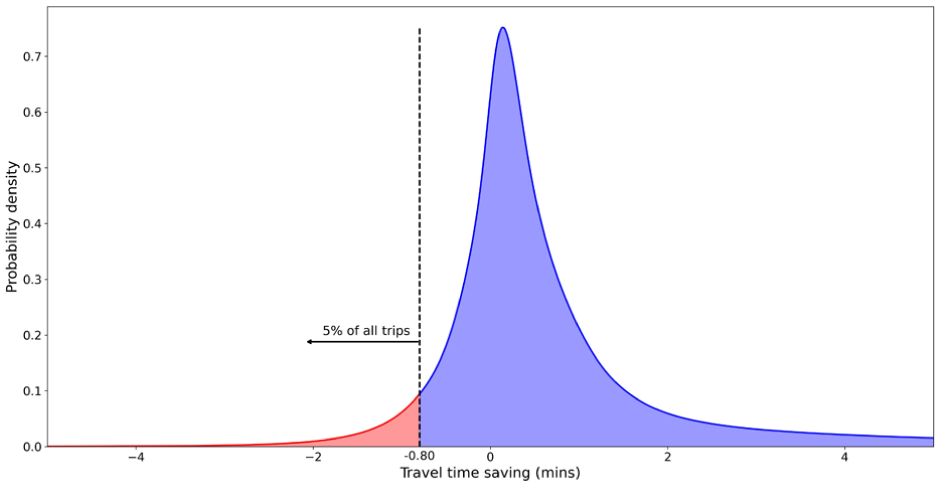
Travel time on GPLs minus travel time on MLs of all trips.

Four personalized variables were created based on each traveler’s trip history within the dataset. The first variable, awareness of slower ML (X_histslowerML), indicates whether a traveler had previously traveled when MLs were slower than GPLs, defined in Equation 1. The second variable, awareness of slower ML by the worst travel time saving (X_{histworstdtime}), represents the maximum travel time difference between MLs minus GPLs in all previous trips for which MLs were slower, defined in Equation 2. The third variable, awareness of slower ML by the worst speed difference (X_{histworstdspeed}), stands for the maximum speed difference between MLs minus GPLs in all previous trips where MLs were slower, defined in Equation 3. Note that travelers did not need to be in MLs to see or experience slower MLs; in other words, GPL travelers could be aware of slower MLs. The last variable, time since the last slower ML trip (X_{timesinceslowerML}), identifies the time gap between the current trip and the last trip a traveler had previously traveled when MLs were slower than GPLs, defined in Equation 4. We had to adjust the X_{timesinceslowerML} owing to the missing data in December 2012 and October 2013. We reset the person time since slower ML to zero for their next observed trip after those 2 months.

X_{histslowerML} = {\begin{matrix} 1; a traveler had previously traveled when MLs were slower than GPLs \\ 0; otherwise \end{matrix}

(1)

X_{histworstdtime} = {\begin{matrix} maximum travel time difference between MLs minus GPLs in all previous trips where MLs were slower \\ 0; a traveler never saw or experienced a situation where MLs were slower \end{matrix}

(2)

X_{histworstdspeed} = {\begin{matrix} maximum speed difference between GPLs minus MLs in all previous trips where MLs were slower \\ 0; a traveler never saw or experienced a situation where MLs were slower \end{matrix}

(3)

X_{timesinceslowerML} = {\begin{matrix} date + time of the current trip - date + time of the last slower ML trip \\ 0; a traveler never saw or experienced a situation where MLs were slower \\ or MLs were slower at the current trip \end{matrix}

(4)

Since variable personalization is less meaningful for occasional travelers, this study focused on regular travelers who averaged at least one trip per month. Owing to the missing data in December 2012 and October 2013, this dataset was segmented into three periods: January 2012 to November 2012, January 2013 to September 2013, and November 2013 to September 2014. Therefore, travelers with the same unique ID who did not meet these thresholds or who did not travel during all three periods were excluded from the analysis. After this filtering process, this dataset contained approximately 48-million trips made by regular travelers, with only 6.95% of those trips on the MLs (see Table 2). The relatively low proportion of ML trips posed potential challenges for the model’s ability to capture ML-related behaviors.

Table 2.

Choosers and Nonchoosers

	Full dataset		Sampling dataset
Traveler group	Trips	Travelers	Sampling, %	Trips	Travelers
Total	48,202,648	226,505	na	380,850	1,610
ML trips	3,350,123	na	na	187,742	na
GPL trips	44,852,525	na	na	193,108	na
ML trip percentage	6.95	na	na	49.30	na
Choosers	31,402,846	128,499	na	251,534	927
Choosers (ML trips ≥ GPL trips)	1,621,094	5,713	10.00	164,887	571
Choosers (ML trips < GPL trips)	29,781,752	122,786	0.29	86,647	356
Nonchoosers	16,799,802	98,006	na	129,316	683
ML nonchoosers	128,998	586	50.00	62,976	293
GPL nonchoosers	16,670,804	97,420	0.40	66,340	390

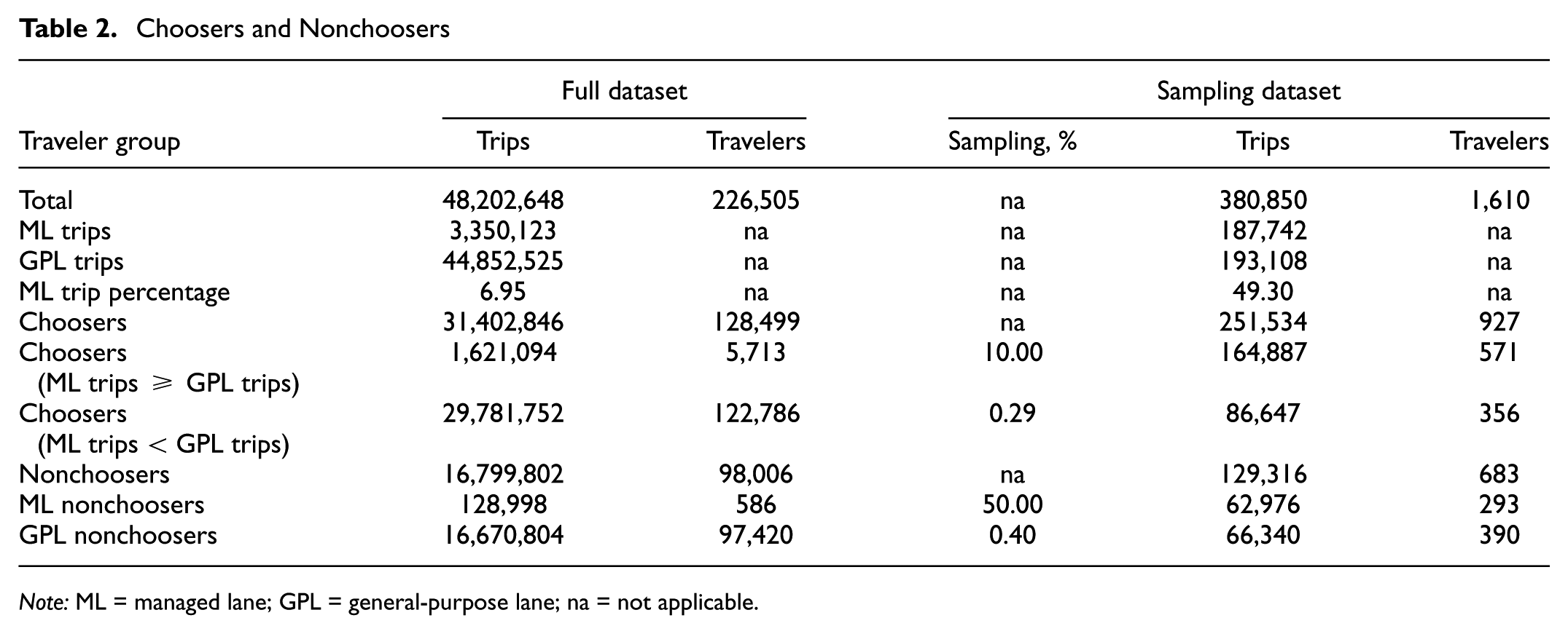
Note: ML = managed lane; GPL = general-purpose lane; na = not applicable.

To address these issues, we classified travelers into four subgroups and then implemented a stratified random sampling approach to represent the whole population and ensure a balance of ML and GPL trips. Travelers were first categorized into two groups based on their lane choice behavior: choosers and nonchoosers. Travelers, referred to as nonchoosers, always use the same lane (always ML or always GPL) regardless of toll rates or time savings. Choosers are those who use both lane types at least once ( 2 , 3 , 24 ). Nonchoosers were further divided into two subgroups based on their lane type: ML nonchoosers and GPL nonchoosers. Choosers were similarly divided based on their predominant usage pattern: choosers with fewer ML trips than GPL trips, and choosers with as many or more ML trips than GPL trips. Then, stratified random sampling was conducted using unique traveler IDs, with different sampling rates applied to each subgroup. Table 2 exhibits the number of trips, number of travelers, and sampling percentages for each subgroup.

Since nonchoosers always make the same decision, they potentially muddle any choice-based model. This study developed two models: all-travelers and choosers-only, which excluded nonchooser travelers. We utilized four alternative-specific variables and eight individual-specific variables to model travelers’ decisions between ML and GPL. Alternative-specific variables included the toll paid, travel time, travel time variability, average speed, and speed variability. Individual-specific variables contained the freeway distance, peak hours, shoulder hours, freeway frequency, awareness of slower ML, awareness of slower ML by the worst travel time saving, awareness of slower ML by the worst speed difference, and time since the last slower ML trip (see Table 3).

Table 3.

Variables

Variable	Data type	Value	Average value or (percent of trips)
Variable	Data type	Value	All-travelers	Choosers-only
ML lane use	Binary	1 = Yes	(49.30%)	(49.60%)
Toll	Continuous	$	1.66	1.71
ML time	Continuous	min	7.86	8.63
GPL time	Continuous	min	9.51	10.41
ML time variability	Continuous	min	0.48	0.54
GPL time variability	Continuous	min	0.80	0.87
ML speed	Continuous	mph	63.17	62.45
GPL speed	Continuous	mph	54.83	54.74
ML speed variability	Continuous	mph	3.91	3.84
GPL speed variability	Continuous	mph	4.96	4.87
Distance	Continuous	mi	7.81	8.45
Peak	Binary	1 = Yes	(25.11%)	(25.59%)
Shoulder	Binary	1 = Yes	(16.74%)	(17.31%)
Frequency	Ordinal
Infrequent (1–3 per month)		1	(10.15%)	(6.92%)
Sometimes (4–12 per month)		2	(44.87%)	(43.12%)
Commuter level 1 (13–29 per month)		3	(40.69%)	(45.04%)
Commuter level 2 (30 or more per month)		4	(4.29%)	(4.93%)
HistslowerML	Binary	1 = Yes	(80.29%)	(85.33%)
Histworstdtime	Continuous	min	3.32	3.57
Histworstdspeed	Continuous	mph	16.11	17.42
TimesinceslowerML	Continuous	day	26.32	28.12

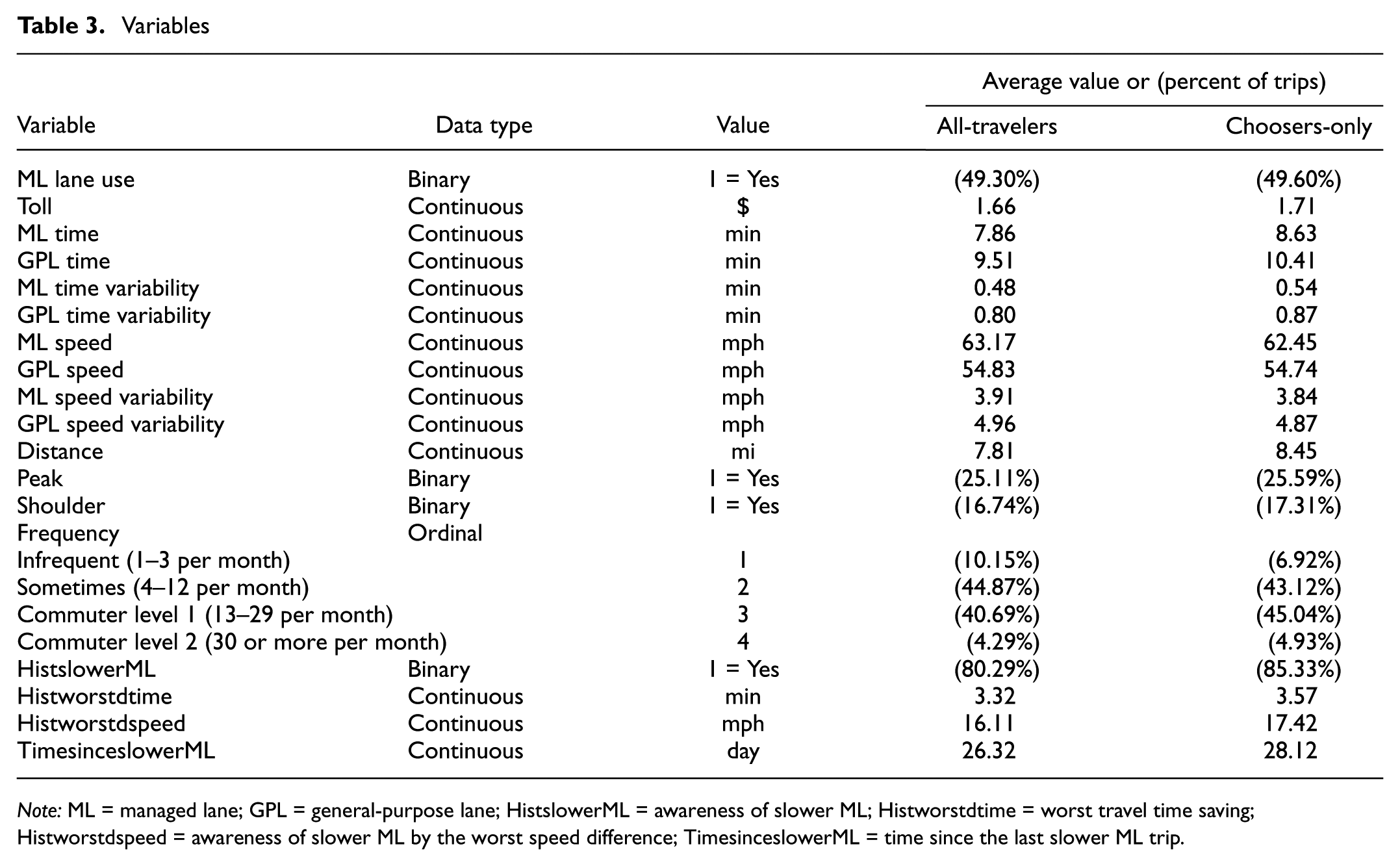
Note: ML = managed lane; GPL = general-purpose lane; HistslowerML = awareness of slower ML; Histworstdtime = worst travel time saving; Histworstdspeed = awareness of slower ML by the worst speed difference; TimesinceslowerML = time since the last slower ML trip.

Logit Choice Model with Random Utility Maximization

Choice models are widely used in the analysis of traveler decisions and travel forecasts. They are employed to gain a deeper understanding of how traveler and trip characteristics affect traveler behavior ( 16 ). They combine microeconomic theory of consumer behavior, psychological choice behavior, and the RUM analysis techniques. The RUM assumes that an individual chooses the choice that offers them the highest utility ( 15 ). As defined in Equation 5, the utility ( $U_{ik}$ ) consists of two components: the observed or deterministic component ( $V_{ik}$ ), derived from alternative-specific or individual-specific variables, and the unobserved or random component ( $ε_{ik}$ ) ( 25 – 28 ).

U_{ik} = V_{ik} + ε_{ik} = V (β X_{ik}) + ε_{ik}

(5)

where

$U_{ik}$ = utility of choice, $k$ , of an individual, $i$ ,

$X_{ik}$ = a vector of variables of choice, k, of an individual, $i$ , and

$β$ = utility coefficients for estimation.

To model lane choice, we utilized a logit model to forecast whether a traveler chose GPLs or MLs. The logit model assumes that $ε_{ik}$ is independently and identically distributed as Type I extreme value (Gumbel). A logit function was adopted as defined in Equation 6 to calculate the ML probability ( $P_{iML}$ ) that individual $i$ chose the MLs ( 14 , 29 ). Lane use is a binary dependent variable and is equal to 1 when a traveler chooses ML. Since we considered the GPL as a base choice, the GPL coefficients $(β_{GPL})$ for individual-specific variables were excluded from the model.

P_{iML} = \frac{e^{V_{iML}}}{e^{V_{iML}} + e^{V_{iGPL}}}

(6)

To identify the best model, we initially included all variables presented in Table 3 in a model. Then, we employed an iterative process to remove variables that were not statistically significant and did not contribute to model improvement. Variables highly correlated with one another were not included simultaneously in the same model. For the model evaluation, we computed log-likelihood, Akaike information criterion, and ρ-squared to measure the goodness of fit of the model. A confusion matrix was generated to check for any models that did a poor job predicting any specific choice.

Results and Discussion

Results

This study developed all-travelers and choosers-only models with the RUM-based logit to forecast drivers’ likelihood of choosing to pay for MLs. Both models demonstrated comparable predictive performance and identified the same set of statistically significant variables: toll, speed, ML travel time variability, awareness of slower ML, and time since the last slower ML trip (see Table 4). In both models, higher tolls and faster ML speeds increased the probability of choosing MLs, whereas seeing or experiencing slower ML travel discouraged future ML use. A longer period since the last slower ML event corresponded to a higher likelihood of ML selection.

Table 4.

Model Results

Variables	All-travelers		Choosers-only
Variables	Coefficients	p-value	Coefficients	p-value
ML constant	−1.26	<2.2e-16	−1.44	<2.2e-16
Toll	0.76	<2.2e-16	0.66	<2.2e-16
Speed	0.03	<2.2e-16	0.04	<2.2e-16
ML time variability	0.28	<2.2e-16	0.57	<2.2e-16
ML histslowerML	−0.33	<2.2e-16	−0.23	<2.2e-16
ML timesinceslowerML	0.001	<2.2e-16	0.002	<2.2e-16
Number of trips	380,850		251,534
LL	−207,630		−136,060
AIC	415,275		272,142
ρ-squared	0.2134		0.2196
Accuracy percentage (%)	71.47		71.88

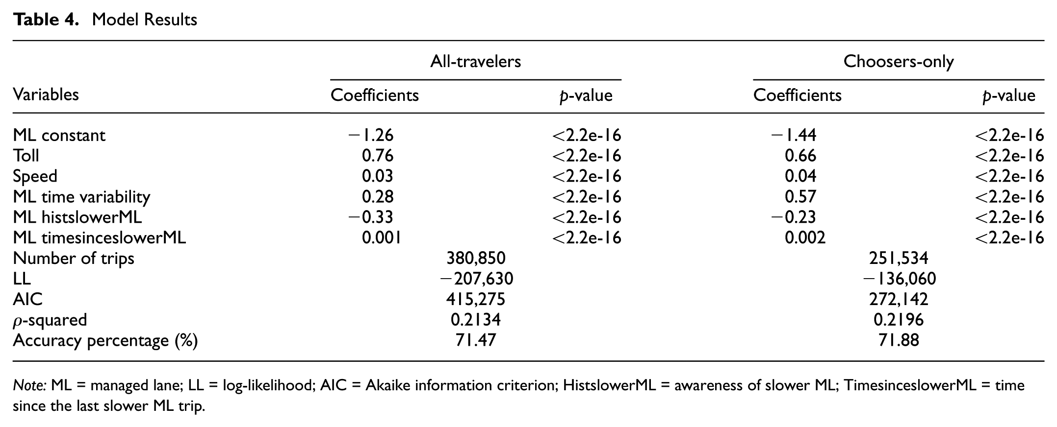
Note: ML = managed lane; LL = log-likelihood; AIC = Akaike information criterion; HistslowerML = awareness of slower ML; TimesinceslowerML = time since the last slower ML trip.

Aside from the RUM-based logit model, we explored several advanced discrete choice modeling techniques, including the mixed logit model ( 16 , 30 ), latent class logit model ( 31 ), cross-nested logit model ( 32 , 33 ), and random regret minimization (RRM)-based logit model ( 28 , 34 ). However, these models did not result in a substantial improvement in predictive performance, and some encountered convergence issues. The mixed logit model did not improve model performance, consistent with the findings reported by Xie et al. ( 7 ). This model also required over 4 h for estimation, indicating a significant computational burden without corresponding gains in model quality. Both latent class logit and cross-nested logit models failed to converge. Additionally, the RRM-based logit model delivered the same performance as the RUM-based logit model but took approximately three times the computational time.

Discussion

Interestingly, travelers tended to use MLs as toll rates increased ( $β_{toll}$ = 0.76 for all-travelers and $β_{toll}$ = 0.66 for choosers-only). This behavior appears counterintuitive when considered through traditional economics theory, where higher prices suppress demand. This finding contrasts with several previous ML studies, which typically report a negative relationship between toll rates and ML demand. However, a similar phenomenon has been observed in the MnPASS HOT lanes in Minnesota. Travelers may perceive higher tolls as a signal of downstream congestion, which encourages them to use MLs to save time ( 35 ). However, the MnPASS HOT lanes employ dynamic pricing, with tolls adjusted to maintain free-flow conditions, whereas the Katy Freeway in this study used variable pricing based on a predetermined schedule. Furthermore, the distribution of toll rates by lane usage in this study showed that higher tolls were clearly associated with a greater number of ML trips. Similarly, the results showed that travelers tended to use MLs more frequently as variability in travel time on MLs increased ( $β_{timevariability}$ = 0.28 for all-travelers and $β_{timevariability}$ = 0.57 for choosers-only). This pattern diverges from findings in the literature, which generally suggest that travelers select MLs to achieve greater travel time reliability ( 5 , 6 ).

One explanation is that travelers prefer to use the MLs during peak periods. Peak hour is when drivers need MLs the most since these periods typically experience the most severe traffic conditions. Given the high variability in travel times during peak hours, travelers may intuitively perceive these periods as an opportunity to take the MLs and obtain the greatest time savings. This is reflected by Katy Freeway’s variable tolling system, where toll rates are adjusted according to a predetermined schedule. Consequently, tolls and travel time variability on MLs are higher during peak hours, reflecting the increased demand for the facility during those times. Since toll values are correlated with time period, we included only toll value in the model.

This study utilized speed rather than travel time to represent traffic conditions along the corridor. This was because toll and travel time were highly correlated but the correlation between toll and speed was acceptable at 0.39 for all-travelers and 0.41 for choosers-only. An additional advantage of using speed is its practical interpretability—drivers can easily observe and assess their speed during a trip. Prior research has also indicated that travelers tend to overestimate travel time savings ( 36 ), making speed a more reliable way for a traveler to judge their GPL versus ML choice. The results suggest that higher speeds in MLs ( $β_{speed}$ = 0.03 for all-travelers and $β_{speed}$ = 0.04 for choosers-only) significantly increased the likelihood of ML selection, supporting the hypothesis that travelers are willing to pay for faster travel.

Lastly, this study highlighted that the instances a traveler saw or experienced slower MLs ( $β_{histslowerML}$ = −0.33 for all-travelers and $β_{histslowerML}$ = −0.23 for choosers-only) affected future lane choice behavior by deterring travelers from using MLs. This suggests a degree of risk aversion in their decision making. Travelers were more likely to pay a toll for ML access when a significant amount of time had passed since the last time they saw or experienced slower MLs ( $β_{timesinceslowerML}$ = 0.001 for all-travelers and $β_{timesinceslowerML}$ = 0.002 for choosers-only). This behavior implies the presence of a forgetting mechanism, wherein awareness of the incident decays over time. In this sense, it aligns with Ebbinghaus’s forgetting curve, which suggests that memory retention declines over time ( 37 ). However, this awareness is likely to be reinforced if the traveler experiences similar ML conditions again.

Conclusion

This study applied a RUM-based logit model to predict individual lane choice decisions and to examine the effect of slower ML incidents on future ML usage. The results indicated that higher tolls and faster MLs increased the likelihood of ML selection, suggesting that travelers are willing to pay more for faster travel. Travelers were more inclined to use MLs when the variability in ML travel time was higher. In contrast, slower travel times on MLs discouraged future use, indicating a degree of risk aversion in traveler behavior. However, this deterrent effect diminished over time, consistent with a forgetting mechanism in which the influence of negative experiences gradually fades. Repeated exposure to similar incidents, on the other hand, reinforces memory and reactivates the deterrent effect. These findings highlight the dynamic nature of traveler decision making, which is influenced not only by present conditions, such as tolls and speed, but also by personal experience over time.

Although this study investigated the impact of slower MLs on future lane choice, it did not account for whether travelers were actually aware of these slower conditions. We assumed that travelers seeing or experiencing a delay of 0.80 min or more were aware of this; however, this assumption lacked direct behavioral validation. Future research should incorporate traveler awareness and perceptions of traffic conditions to improve the accuracy of such models. Slower ML conditions can occur under both variable and dynamic pricing methods, as observed in other ML facilities across the United States. Although it would be valuable to extend this analysis to other facilities beyond the Katy Freeway, few currently have transponder readers installed on GPLs, limiting the availability of comparable data. If toll agencies or state departments of transport begin to install readers along GPLs, researchers will be able to examine traveler behavior across different facilities and pricing methods. Future studies should explore the implications of these pricing mechanisms under such scenarios and evaluate how slower ML performance affects facility use, particularly in systems employing dynamic pricing strategies. Moreover, the time period, such as peak and off-peak periods, may influence travelers’ decisions on MLs. However, in this study, these factors were highly correlated with toll variables and were therefore excluded from the models. In future research, we aim to conduct an analysis that incorporates both the time of day and the current factors to achieve a more comprehensive understanding of travel behavior on MLs. Additionally, the Bayesian updating approach could be applied in future research to investigate the behavior of travelers with limited experience of slower MLs. This approach assumes that travelers do not know a priori the probability that MLs will be slower. When they experience slower MLs, they adjust their subjective probability upward, and when they experience faster MLs, they adjust it downward. This mechanism could provide a rational explanation regardless of whether a traveler is risk-averse, risk-neutral, or even risk-loving.

Footnotes

Acknowledgements

We gratefully acknowledge the Harris County Toll Road Authority, Texas Department of Transportation, and Greater Houston Transportation and Emergency Management Center (Houston TranStar) for providing the Katy Freeway dataset. We appreciate the contributions of several Texas A&M University students, including Sunghoon Lee and A.K.M. Abir for the data cleaning and database development efforts. We thank Texas A&M University’s High Performance Research Computing for providing the computational resources necessary to perform the high-performance analyses conducted in this study.

Author Contributions

The authors confirm contribution to the paper as follows: study conception and design: N. Leungbootnak, M. Burris; data collection: N. Leungbootnak, M. Burris; analysis and interpretation of results: N. Leungbootnak, M. Burris; draft manuscript preparation: N. Leungbootnak, M. Burris. All authors reviewed the results and approved the final version of the manuscript.

Declaration of Conflicting Interests

The authors declared no potential conflicts of interest with respect to the research, authorship, and/or publication of this article.

Funding

The authors received no financial support for the research, authorship, and/or publication of this article.

ORCID iDs

Natchaphon Leungbootnak

Mark Burris

References

TRB Managed Lanes Committee. Projects Database – Managed Lanes. https://managedlanes.wordpress.com/2021/01/05/projects-database/. Accessed June 25, 2025.

Burris

M. W.

Brady

J. F.

Unrevealed Preferences: Unexpected Traveler Response to Pricing on Managed Lanes. Transportation Research Record, 2018. 2672(5): 23–32. https://doi.org/10.1177/0361198118796928.

Ashraf

Brown

A. L.

Burris

M. W.

Vitaku

Aggregate and Individual Effects of Information in a Coordination (Traffic) Game. Economic Inquiry, Vol. 61, No. 4, 2023, pp. 818–850. https://doi.org/10.1111/ecin.13143.

Leungbootnak

Cheung

Pal

Burris

Are Toll Facility Travelers Aware of Their Toll?

Transportation Research Record, Vol. 2679, No. 6, 2025, pp. 171–182. https://doi.org/10.1177/03611981241312921.

Leung

McCartan

Robinson

Kiana

R. Z.

Hallenbeck

Iverson

I-405 Express Toll Lanes Usage, Benefits, and Equity. eScience Institute, Seattle, W. A., 2019.

Brent

D. A.

Gross

Dynamic Road Pricing and the Value of Time and Reliability. Journal of Regional Science, Vol. 58, No. 2, 2018, pp. 330–349. https://doi.org/10.1111/jors.12362.

Xie

Zhang

Akkinepally

A. P.

Ben-Akiva

Personalized Choice Model for Managed Lane Travel Behavior. Transportation Research Record, 2020. 2674(7): 442–455. https://doi.org/10.1177/0361198120923355.

Patil

Burris

Douglass Shaw

Travel Using Managed Lanes: An Application of a Stated Choice Model for Houston, Texas. Transport Policy, Vol. 18, No. 4, 2011, pp. 595–603. https://doi.org/10.1016/j.tranpol.2011.02.004.

Huang

Burris

Shaw

W. D.

Differences in Probability Weighting for Individual Travelers: A Managed Lane Choice Application. Transportation, Vol. 44, No. 2, 2017, pp. 375–393. https://doi.org/10.1007/s11116-015-9642-x.

10.

Sheikh

Guin

Guensler

Value of Travel Time Savings: Evidence from I-85 Express Lanes in Atlanta, Georgia. Transportation Research Record, 2014. 2470(1): 161–168. https://doi.org/10.3141/2470-17.

11.

Sharifi

Burris

M. W.

Application of Machine Learning to Characterize Uneconomical Managed Lane Choice Behaviour. Case Studies on Transport Policy, Vol. 7, No. 4, 2019, pp. 781–789. https://doi.org/10.1016/j.cstp.2019.08.003.

12.

Hossan

M. S.

Asgari

Jin

Investigating Preference Heterogeneity in Value of Time (VOT) and Value of Reliability (VOR) Estimation for Managed Lanes. Transportation Research Part A: Policy and Practice, Vol. 94, 2016, pp. 638–649. https://doi.org/10.1016/j.tra.2016.10.022.

13.

Jin

Hossan

M. S.

Asgari

Investigating the Value of Time and Value of Reliability for Managed Lanes. Florida International University, Miami, FL, Publication BDV29-977–12. 2015. https://rosap.ntl.bts.gov/view/dot/29615.

14.

McFadden

Conditional Logit Analysis of Qualitative Choice Behavior. Academic Press, New York, 1972.

15.

Ben-Akiva

Bierlaire

Discrete Choice Methods and Their Applications to Short Term Travel Decisions. In Handbook of Transportation Science ( Hall

R. W.

, ed.), Springer US, Boston, MA, pp. 5–33.

16.

Train

K. E.

Discrete Choice Methods with Simulation. Cambridge University Press, Cambridge, England, 2009.

17.

Small

K. A.

Winston

Yan

Uncovering the Distribution of Motorists’ Preferences for Travel Time and Reliability. Econometrica, Vol. 73, No. 4, 2005, pp. 1367–1382. https://doi.org/10.1111/j.1468-0262.2005.00619.x.

18.

Toledo

Sharif

The Effect of Information on Drivers’ Toll Lane Choices and Travel Times Expectations. Transportation Research Part F: Traffic Psychology and Behaviour, Vol. 62, 2019, pp. 149–159. https://doi.org/10.1016/j.trf.2018.12.023.

19.

Green

L. L.

Burris

M. W.

Can Psychological Questions Help Predict Managed Lane Use?

Transportation Research Record, 2014. 2470(1): 152–160. https://doi.org/10.3141/2470-16.

20.

Huang

Burris

Shaw

W. D.

Models of Transportation Choice with Risk: An Application to Managed Lanes. Transportation Letters, Vol. 9, No. 5, 2017, pp. 276–295. https://doi.org/10.1080/19427867.2016.1204811.

21.

Mulligan

Katy Freeway. Houston, TX, 2017.

22.

Biswas

Burris

Jha

Holloway

Comparing Pricing Mechanisms for Managed Lanes. Transport Economics and Management, Vol. 2, 2024, pp. 112–121. https://doi.org/10.1016/j.team.2024.05.001.

23.

Lee

Real Option Analysis to Value Managed Lanes Using Big Data. Texas A&M University, College Station, TX, 2016.

24.

Rahman

Burris

Predicting Managed Lane Choice by Integrating Real World Data and Behavioral Science. https://papers.ssrn.com/abstract=5166622. Accessed June 11, 2025.

25.

Louviere

J. J.

Street

Burgess

Wasi

Islam

Marley

A. A. J.

Modeling the Choices of Individual Decision-Makers by Combining Efficient Choice Experiment Designs with Extra Preference Information. Journal of Choice Modelling, Vol. 1, No. 1, 2008, pp. 128–164. https://doi.org/10.1016/S1755-5345(13)70025-3.

26.

Heras-Molina

Gomez

Vassallo

J. M.

Drivers’ Adoption of Electronic Payment in the Spanish Toll Road Network. Transportation, Vol. 46, No. 3, 2019, pp. 931–955. https://doi.org/10.1007/s11116-017-9831-x.

27.

Walker

Ben-Akiva

Generalized Random Utility Model. Mathematical Social Sciences, Vol. 43, No. 3, 2002, pp. 303–343. https://doi.org/10.1016/S0165-4896(02)00023-9.

28.

Enhanced Navigational Insights and Their Impact on Driver Route Choice: A Hybrid Utility-Regret Analysis with Heterogeneity. Research in Transportation Economics, Vol. 110, 2025, p. 101539. https://doi.org/10.1016/j.retrec.2025.101539.

29.

Srisan

Bills

A Case for Race and Space in Auto Ownership Modeling: A Los Angeles County Study. Transport Policy, Vol. 154, 2024, pp. 182–197. https://doi.org/10.1016/j.tranpol.2024.06.006.

30.

Sarrias

Daziano

Multinomial Logit Models with Continuous and Discrete Individual Heterogeneity in R: The Gmnl Package. Journal of Statistical Software, Vol. 79, 2017, pp. 1–46. https://doi.org/10.18637/jss.v079.i02.

31.

Greene

W. H.

Hensher

D. A.

A Latent Class Model for Discrete Choice Analysis: Contrasts with Mixed Logit. Transportation Research Part B: Methodological, Vol. 37, No. 8, 2003, pp. 681–698. https://doi.org/10.1016/S0191-2615(02)00046-2.

32.

Lemp

J. D.

Kockelman

K. M.

Damien

The Continuous Cross-Nested Logit Model: Formulation and Application for Departure Time Choice. Transportation Research Part B: Methodological, Vol. 44, No. 5, 2010, pp. 646–661. https://doi.org/10.1016/j.trb.2010.03.001.

33.

Bierlaire

BIOGEME: A Free Package for the Estimation of Discrete Choice Models. Presented at the Swiss Transport Research Conference, Monte Verità, Ascona, Switzerland, 2003.

34.

Chorus

C. G.

Random Regret-Based Discrete Choice Modeling: A Tutorial. Springer Science & Business Media, Heidelburg, Germany, 2012.

35.

Janson

Levinson

HOT or Not: Driver Elasticity to Price on the MnPASS HOT Lanes. Research in Transportation Economics, Vol. 44, 2014, pp. 21–32. https://doi.org/10.1016/j.retrec.2014.04.008.

36.

Devarasetty

P. C.

Burris

Chao

Comparing Perceived and Actual Travel Time Savings on Freeways with Managed Lanes. The Journal of Transportation of the Institute of Transportation Engineers, Vol. 6, 2014, pp. 1–13.

37.

Ebbinghaus

Über das Gedächtnis: Untersuchungen zur experimentellen Psychologie. Duncker & Humblot, Leipzig, Germany, 1885.

The Effect of Slower Managed Lanes on Future Lane Choice

Abstract

Keywords

Introduction

Literature Review

Modeling Lane Choice: Methodology

Katy Freeway

Data Collection

Data Preprocessing

Logit Choice Model with Random Utility Maximization

Results and Discussion

Results

Discussion

Conclusion

Footnotes

Acknowledgements

Author Contributions

Declaration of Conflicting Interests

Funding

ORCID iDs

References