
Abstract
Roadway performance models are one component of travel demand model systems, whose primary purpose is to replicate the congestion effect in traffic assignment. In this sub-model, accurate estimates of roadway travel time (delay), which is sensitive to road traffic volumes, have a principal role in properly assigning trips from origin zones to destination zones to various paths through the road network. One of the main challenges of developing these volume-delay models is the availability of data, which historically was largely lacking. Thanks to emerging data sources, the speed and volume for a wide range of roadway segments in the network are available in excellent temporal and spatial resolution. This study proposes a multi-stage machine-learning-based framework to clean, classify and calibrate roadway performance models of various roadway functional classes in the Greater Toronto and Hamilton Area (GTHA). Recurrent spatial and temporal trends of roadway performance are further investigated, and distinctive patterns are observed for road segments with specific physical attributes.
Keywords
Traffic congestion is a pressing issue in urban areas, causing productivity losses and increased travel times. This arises as a result of excessive traffic demand on limited road capacity. To tackle this problem effectively, a comprehensive approach is necessary, examining both transportation demand and infrastructure supply. To address congestion in cities, planners and decision-makers require a reliable tool to assess local transport needs and guide policy changes and infrastructure investments. Travel demand models serve this purpose by predicting future travel patterns through “what if” scenarios, analyzing hypothetical interactions between travel demand and network supply. These models consist of mathematical algorithms, culminating in the trip assignment phase, where the most computationally intensive calculations occur. This step captures the interplay between travel demand and transportation supply, generating performance measures for policy evaluation. For the Greater Toronto-Hamilton Area (GTHA), the GTAModel is an activity-based, agent-based microsimulation model, connected to Emme software for traffic and transit assignment. Utilizing evidence-based tools like these will enable informed decisions to alleviate traffic congestion and enhance urban mobility.
Among the performance measures generated by travel demand models, travel time stands out as the most crucial. It, along with other related metrics like vehicle kilometers traveled (VKT), plays a vital role in evaluating mobility, accessibility, congestion, economic benefits, and environmental impacts of transportation improvement projects. Travel time is determined using the volume-delay function (VDF), which predicts average link travel time as a function of link flow at a given point in time. This function considers variables like traffic flow (resulting from assignment), link distance, free flow speed, capacity, and a speed–flow relationship.
Despite significant technological advancements in transportation systems and travel modeling, the VDF, developed in the 1960s, has seen minimal modifications. Researchers tend to favor roadway performance models that better represent vehicle queuing, such as those in dynamic traffic assignment, whereas transportation planners still rely on traditional and simplistic methods like the Bureau of Public Roads (BPR) function for static traffic assignments. To bridge this gap between research and practical application, in this study, a data-driven pipeline is prepared to cluster and calibrate roadway performance models used in both static and dynamic traffic assignments, ultimately meeting the expectations of both researchers and planners.
The effectiveness of travel demand models depends on accurate calibration and implementation of transportation supply and demand within the overall modeling framework. While the demand side calibration in the GTHA has been a significant endeavor, the supply side is often left uncalibrated because of data scarcity. In Toronto, the last calibration occurred in 1992, assuming constant speed–flow relationships and parameters for each road functional class without empirical measurements ( 1 ). This approach overlooks the variations in volume–delay characteristics, leading to the adoption of a general VDF for the entire city, only categorized, at most, by road functional class.
To address these issues, this study focuses on calibrating and clustering VDFs for the GTAModel-based Emme assignment in the GTHA. As one of North America’s largest metropolitan areas, the GTHA faces challenges such as air pollution, housing shortages, and health care, with significant travel demand and traffic congestion on its transportation networks. Investments in transportation infrastructure have been made, but scrutiny of transportation plans and policies is necessary to ensure benefits without adverse consequences, particularly with regard to traffic congestion.
Emerging data sources like global positioning system (GPS)-enabled devices provide vast digital footprints, offering opportunities to calibrate travel demand models using these passive location traces. The study utilizes the Streetlight Data analytics platform to access comprehensive data for evaluating transportation infrastructure performance under various conditions.
The research aims to develop a simplified yet realistic transportation performance model to aid planners in gaining insights into the transportation system’s performance and devising robust and adaptive plans. By using a data-driven approach and a multi-stage clustering and calibration framework, the study seeks to create transportation performance models with broader applicability and spatial transferability. Ultimately, this research can help bridge the gap between academic and operational use of transportation supply models and contribute to better transportation planning and decision-making.
Literature Review
Transportation planning critically hinges on accurate representations of traffic flow and congestion. The VDF is an essential tool used in traffic assignment models to capture the relationship between traffic volume and travel time ( 2 ). This literature review explores the complexities of VDF calibration, with a special focus on its definition, different models, limitations, influencing factors, and calibration techniques. The importance of continuous research and refinement of VDFs will also be discussed, alongside the application of machine learning techniques in traffic condition clustering.
VDFs play a crucial role in traffic studies and planning, as they establish a relationship between traffic volume and delay. The volume represents the level of traffic demand, while delay denotes the decrease in traffic speeds as demand increases. To calculate delay accurately, a temporal baseline is required, and in the context of vehicular journey time, this baseline is the free flow condition of the roadway. When traffic demand surpasses the free flow threshold, congestion occurs, leading to queues and delays for drivers.
Over time, various formulations of VDFs have been proposed based on theoretical and empirical backgrounds ( 3 ). Early models, such as the linear function proposed by Irwin et al. ( 4 ) and the complex forms by Mosher ( 5 ), Overgaard ( 6 ), and Smock ( 7 ), aimed to better represent traffic behavior. Notably, the BPR and Davidson functions from the 1960s have garnered significant attention and discussion in the field ( 8 , 9 ).
VDFs, developed through mathematical or theoretical methods, play an essential role in replicating traffic behavior and travel demand models. They facilitate travel time minimization problems during traffic assignment ( 10 ) by calculating total path costs, thus ensuring a balance in competing paths for user equilibrium.
Despite their utility, VDFs possess limitations. They oversimplify traffic dynamics and inadequately represent actual volumes and travel times ( 11 , 12 ). They overlook intersection delays, different vehicle speeds, and geometry changes. Additionally, they show scaling inconsistencies, time-of-day insensitivity, and struggle with over-capacity volumes and applying turn penalties ( 13 ).
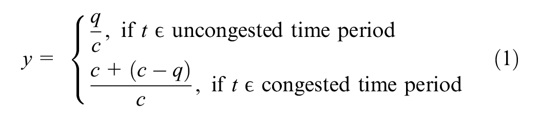
General volume-delay functions are basically defined as the following formulation:
VDFs are influenced by various factors, capturing the effect of congestion on travel time. Besides the number of vehicles on the road, other elements affect travel time, as identified by the Federal Highway Administration (FHWA). These include bottlenecks, poor signal timing, special events, construction zones, severe weather, and traffic accidents. Additionally, physical and operational characteristics of the road environment and users, such as vehicle type, road layout, geometry, and land use, also play a role. Vehicle type diversity can lead to varying speeds and interactions, particularly with heavy trucks causing congestion ( 17 ). Weather conditions like rain or snow can reduce traffic speed significantly ( 18 ). Road incidents, such as roadworks or crashes, can disrupt capacity, leading to longer travel times. The road layout, geometry, and land use also impact vehicle interactions and speed.
Calibration is a crucial process in obtaining mathematical expressions from real-world data for roadway performance metrics. Nonlinearity, heteroskedasticity, and site-specificity must be considered. Nonlinearity means that the rate of change of travel time delay varies with the level of traffic flow, while heteroskedasticity deals with speed variance because of stochastic vehicular interactions. Site-specificity involves calibrating speed–flow data for various road segments in the study area. VDF calibration comprises two steps: selecting a proper formulation and statistically estimating its parameters. Challenges arise in measuring demand in congested regimes, where theoretical approaches, bottleneck analysis, and queue length estimation are used ( 19 ). Mapping speed–flow data between observable and unobservable congested regimes poses the main challenge. Various methods to calibrate VDFs include volume-based method (VBM) ( 20 ), density-based method (DBM) ( 21 ), queue demand-based method (QBM) ( 22 ), time-dependent queue-based D/c (demand-to-capacity ratio) method (TDQDC) ( 19 ), and time-dependent cumulative demand flow-based travel time method (TDCD) ( 23 ) utilizing flow, density, and queue data for different congestion scenarios.
The VBM is taken from the Florida Standard Urban Transportation Modeling Structure (FSUTMS) ( 20 ). In the congestion regime, this method mirrors the speed–flow data point by v/c = 1 line (Equation 1).
In DBM, the travel time–flow calibration of VDF turns into travel time–density estimation. This has been done because the speed–density relationship is monotonic in congested cases, which resembles the same form as the delay–volume curve. Kucharski and Drabicki ( 21 ) used the hydrodynamic relation of the fundamental diagram to calculate quasi-density from time–mean speeds and flows. Therefore, the transformation of volume over the capacity ratio to the quasi-density ratio will be as Equation 2:

where
Wu et al. ( 22 ) proposed a peak-period-based calibrating framework (QBM) based on the freeway bottleneck modeling perspective (Equation 3).

where
Huntsinger and Rouphail ( 19 ) proposed a TDQDC model to estimate the demand beyond capacity as Equation 4:
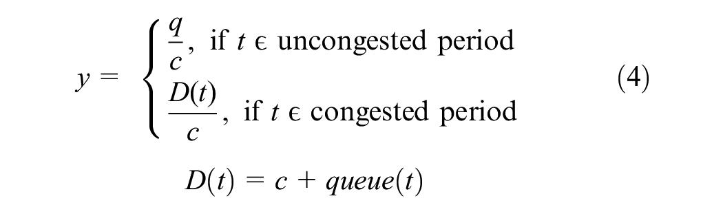
where
The TDCD method is a rolling horizon model which generates one sample point for each interval. Its formulation is as Equation 5 ( 23 ):
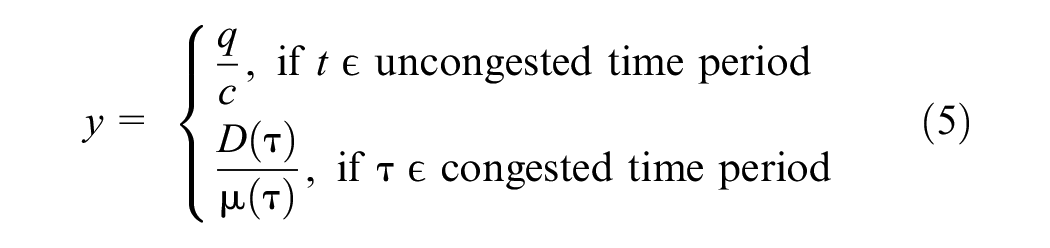
where
Inaccuracies in VDF calibration can stem from sample selection bias, the functional form of the model, observed data variance, and singular value estimation. To address these issues, low volume data sampling and weighting strategies can be used. Testing various mathematical forms on the data helps find the best-fit model. Incorporating speed variance as weights in the weighted least square method considers heteroskedasticity. Joint estimation of speed–flow–density relationships can enhance calibration accuracy.
Traffic flow fundamental diagram is critical in traffic flow theory, serving as the foundation for kinematic wave models, hydrodynamic models, and other traffic-related analyses. These functions depict the relationship between traffic flow rate, density, and speed. Greenshields et al.’s ( 24 ) linear model was one of the first to describe the relationship between these variables, laying the groundwork for future studies. Greenberg ( 25 ) offered a different perspective with a logarithmic approach, providing an alternative way to understand traffic behavior. However, these early models had limitations, often unable to effectively represent multi-regime dynamics or adapt to varying traffic conditions. Researchers like Drew ( 26 ) and Underwood ( 27 ) sought to enhance these models by introducing additional parameters, yet they still fell short of capturing complex traffic patterns. The triangular model by Newell ( 28 ) and Daganzo’s ( 29 ) trapezoidal model marked a shift toward greater flexibility, allowing for more accurate transitions between traffic regimes and providing a broader range of characteristics to represent traffic flow. The constant evolution of traffic patterns, driven by urbanization and changing transportation infrastructure, suggests a need for further refinement of flow–density models to better adapt to diverse traffic conditions, enabling more effective traffic management systems.
Various studies have applied unsupervised machine learning methods to cluster traffic conditions. Azimi and Zhang ( 30 ) compared K-means, fuzzy C-means, and CLARA algorithms on speed–flow data, with K-means showing better consistency with HCM level of service criteria. Neural network pattern recognition was employed by Yang and Qiao ( 31 ) for clustering Chinese highway traffic flow conditions. Sun and Zhou ( 32 ) used K-means to cluster speed–density data, aiding in determining breakpoints in multi-regime traffic models. Xia and Chen ( 33 ) developed an agglomerative clustering method with BIC and dispersion measurements to determine the optimum number of clusters for freeway conditions. Density’s significant effect on clustering results was highlighted by Xia and Chen ( 34 ). Kianfar and Edara ( 35 ) compared clustering algorithms, concluding that K-means and hierarchical clustering outperformed GMM. Xia et al. ( 36 ) proposed an online identification approach using modified agglomerative clustering, while Gu et al. ( 37 ) used a big data-driven two-stage framework for clustering link fundamental diagrams and road functional classes. Finally, Wang et al. ( 38 ) applied mixture model-based clustering for network-level simulation calibration, highlighting potential challenges with heuristic clustering on overlapping data.
Data Sources
The primary data source used in this study is the speed–flow data exported from the StreetLight Data platform. In addition, GTAmodel V4.2 travel demand model output and DMTI land-use data are also used in the study.
StreetLight Data
As a result of recent breakthroughs in information and communication technology, the use of real-time crowd-sourced data feeds in transportation modeling has increased. These novel data sources have wider spatial coverage compared to conventional traffic data sources. In this research project, the research team obtained an academic license from StreetLight Data, which is an on-demand mobility analytics platform. StreetLight Data leverages its cutting-edge data processing engine, Route Science®, to convert extensive raw location data into actionable insights. Each month, Route Science® handles over 40 billion anonymized location records sourced from smartphones, navigation devices, and connected vehicles. Utilizing advanced algorithms, the engine meticulously cleans, aggregates, and normalizes the data, revealing insightful travel patterns. Rigorous validation against diverse external sources, including permanent and temporary sensors, household surveys, and the Census, results in accurate and reliable metrics. In this study, 15 min vehicular traffic counts and average speed were obtained from the Streetlight platform for selected road segments in the GTHA. Having data for 3 months from 791 road segments in the GTHA provides an excellent view of the temporal variations and trends exhibited in the region’s road infrastructure. Depending on the road functional classifications, data quality and availability may vary. The reason for this might be that on some roadways, just a few or no cars traversing a section of the road may be recorded.
GTAModel V4.2 Outputs
GTAModel V4.2 is the latest operational version of the integrated activity-based travel demand model that is used to study and anticipate travel patterns in the GTHA. The Travel Modelling Group (TMG) created this model, which is continually being updated ( 39 ). GTAModel generates complete 24 h weekday travel patterns, among which the a.m. peak period (6:00–9:00 a.m.) is the focus of this study. From various outputs of this travel demand model, the roadway saturation rate (volume over capacity ratio) is employed in this study. This measure is calculated using GTAModel-based EMME road and transit assignment software.
Road Network and Street Attributes
The GTHA 2016 EMME network was developed by TMG and its partners. The information concerning the attributes of elements in this network is documented in the Network Coding Standard (NCS) ( 40 ), which is updated every five years when the region’s Transportation Tomorrow Survey (TTS) is undertaken. The EMME network contains nodes, links and transit lines, from which the links are the focus of the study. Some attributes are assigned to each link, including link, length, number of lanes, functional class, speed, lane capacity, and lane type. It should be noted that for each functional class, a specific volume-delay function is defined. The functional classes in NCS16 (The 2016 Network Coding Standard, developed by the University of Toronto Travel Modelling Group for use by member agencies in the GTHA.) are derived from the combination of multiple sources: NCS11, geometric design guide and GGHMv4 (The Greater Golden Horseshoe Model, Version 4, developed by the Ontario Ministry of Transportation.) VDF definitions. Table 1 shows the link functional classes and VDF definitions in the NCS16. The GTAmodel Emme network has 50691 road segments that are clustered into 18 classes.
Link Functional Class and Volume-Delay Function (VDF) Definitions, Source: UofT Travel Modelling Group (TMG) ( 40 )
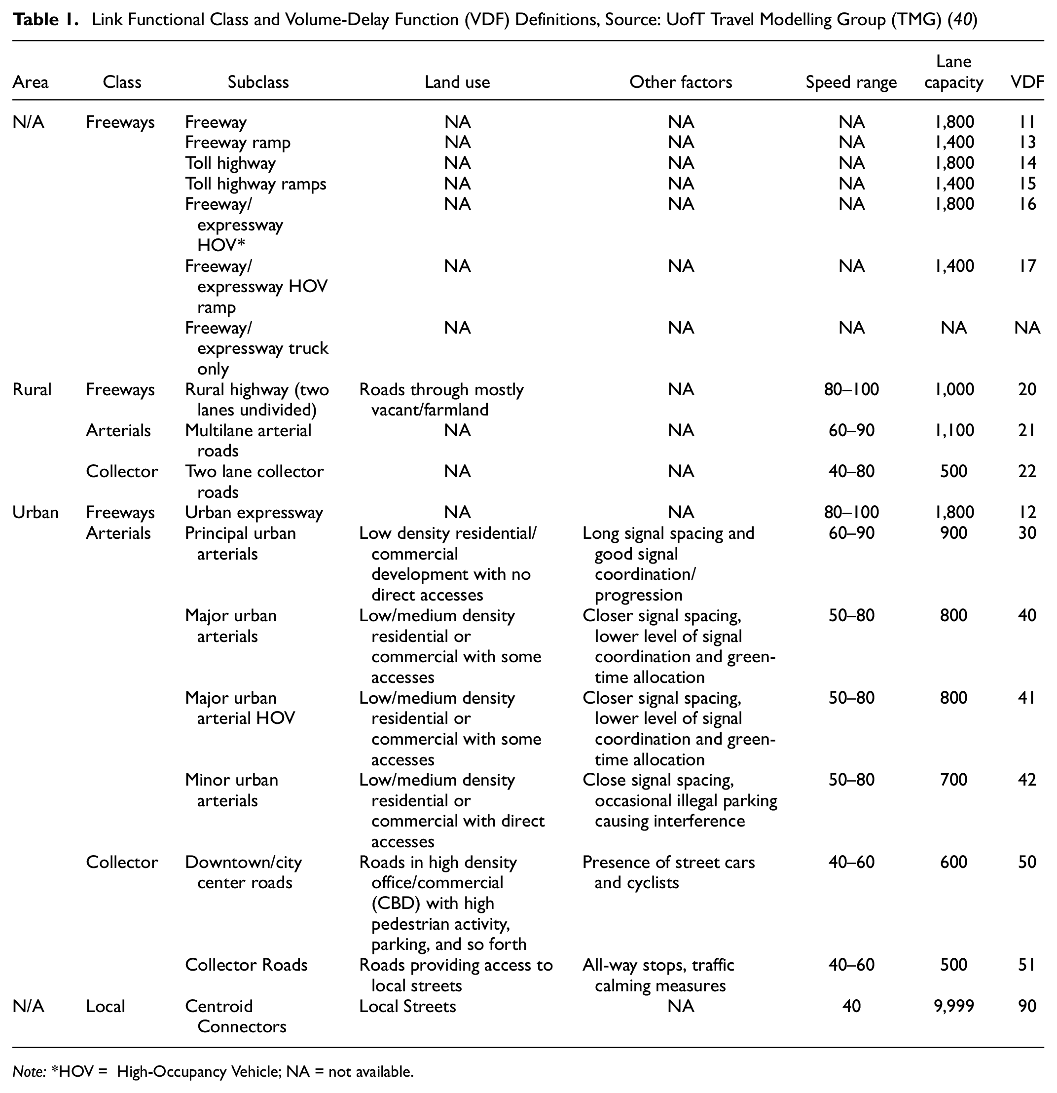
Note:*HOV = High-Occupancy Vehicle; NA = not available.
DMTI Land-Use Data
This analysis makes use of the Desktop Mapping Technologies Inc. (DMTI) land use dataset, which contains historical data on land use patterns at the dissemination area (DA) scale. The land-use percentage within a DA is divided into the following categories: residential, commercial, institutional, industrial, parks, open space, and water. This dataset contains 2001, 2006, 2011, and 2016. The latest year is used for the analysis. The DMTI land use data are spatially joined on the GTAmodel road network. When a road segment crosses several land-use areas, the land use allocated to that road segment is averaged over the intersecting region.
Methodology
Calibration Framework Structure and Specifications
To replicate the true potential of transportation infrastructure supply, the analysis should be done on a typical day that has normal traffic operating conditions. To account for long-term planned and unexpected short-term incidents, a multi-step machine learning-based framework is proposed to clean, classify, and calibrate traffic flow fundamental diagrams of various roadway functional classes in the GTHA. This framework is formed by three clustering algorithms that detect typical days, normal traffic conditions, and road functional classes in three consecutive stages. In the last stage of the framework, the cleaned and clustered data are utilized for VDF calibration. Figure 1 presents the framework mentioned above.
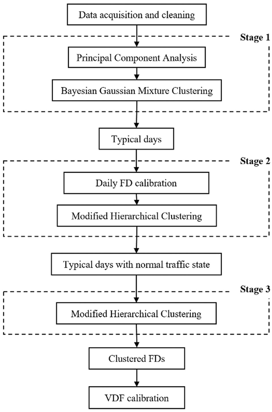
Three-stage clustering and calibration framework.
Data acquisition and data cleaning are the preliminary steps of this framework. One morning peak hour run of the existing GTAModel-based Emme assignment is used to identify the road segments for data acquisition from StreetLight Data. Although the GTAModel’s existing volume-delay function is not well calibrated, the traffic assignment that uses the existing VDFs can provide an initial suggestion for selecting a congested road segment for further VDF calibration. Congested road segments are chosen based on a volume-to-capacity ratio. 791 road segments are selected from the 3,642 road segments that have v/c greater than 0.9 in the network, which is shown in Figure 2. The reason for selecting the existing congested roadway is that we need to find the road segments that contain a wide range of data points of congested and uncongested traffic conditions across each day, which is necessary for avoiding sample selection bias in calibrating the VDF parameters.
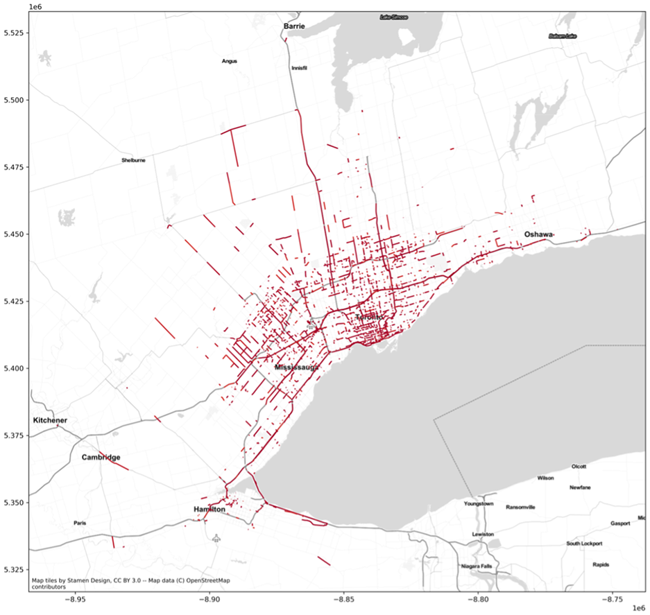
GTAModel Emme-based road segments with volume (v) / capacity (c) > 0.9.
After gathering the two primary traffic flow variables from the StreetLight platform, initial data cleaning is required. For instance, speed–flow pairs with a density lower than 5 vehicles per kilometer per lane (vpkpl) and speed lower than 95% of the maximum speed are deleted to eliminate the heavy trucks that have low speeds at night. Additionally, data points containing only one variable from speed and flow are filtered out.
For each road segment per day, we have at most 96 15 min-aggregated speed–flow pairs, which means a maximum of 192 features per day. The daily feature count may vary by day and road functional classes because GPS-equipped vehicles may not traverse the roadway during some times of the day.
The raw speed–flow data points display wide variability. There are varieties of incidents that result in traffic state variation, from short-term unexpected to long-term planned incidents. To filter long-term planned incidents and find the typical days, principal component analysis (PCA) combined with Bayesian Gaussian mixture clustering is used. For each road segment, each day with a maximum of 192 possible features is imported into the PCA. PCA is used to reduce the dimension of feature space while keeping most of the information contained in the data. After visually inspecting the elbow method in Figure 3 for a sampled road segment, the first two principal components have been chosen. This decision is grounded in their ability to collectively account for approximately 50% of the cumulative explained variance in the data.
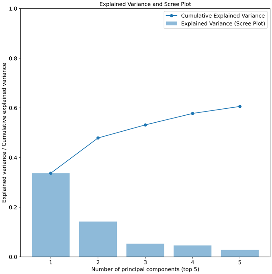
Principal component analysis (PCA) explained variance and scree plot.
The score and loading plots for the first and second principal components are shown in Figure 4. The data points (dates) are represented as black dots in the biplot. The variables (features) from the dataset are represented as red (speed at different times of day) and blue (volume at different times of day) arrows in the biplot. (Color online only.)
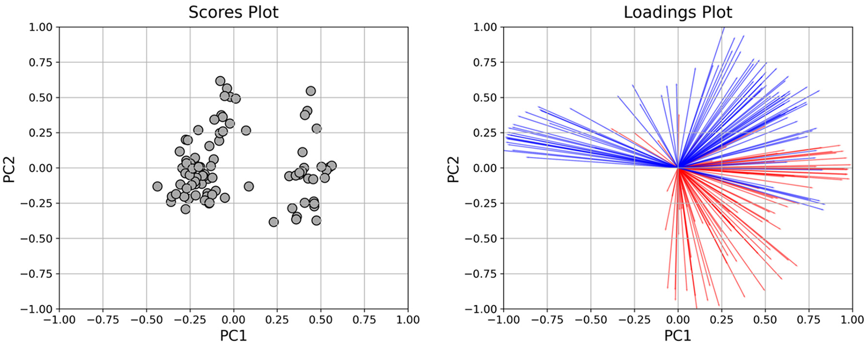
Principal component analysis (PCA) scores–loadings biplot.(Color online only.)
Figure 5 illustrates the foremost 15 influential factors for PC1 (Principal Component 1) and PC2 (Principal Component 2). In a straightforward interpretation, PC1 predominantly reflects the speed and flow during the early morning peak, whereas PC2 depicts similar parameters for the evening peak.
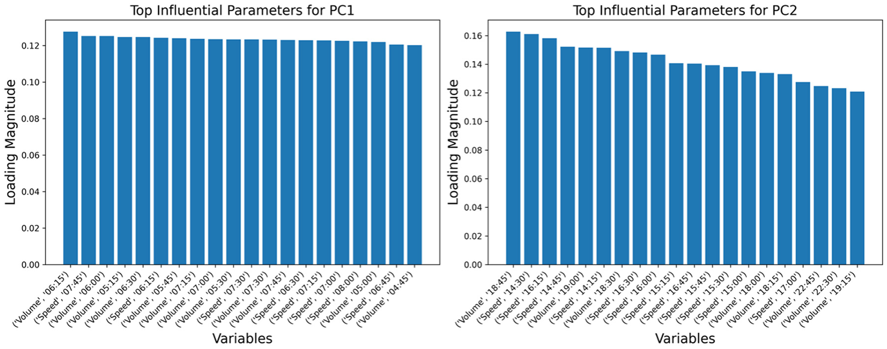
Top influential parameters for PC1 (Principal Component 1) (left) and PC2 (Principal Component 2) (right).
After reducing the dimension of this feature vector, a clustering method was applied to build and find the clusters with different types of days. On the first and second components of PCA, several centroid-/density-/distribution-based clustering methods were applied and assessed, and the distribution-based technique was shown to be the most effective. To be more specific, Bayesian Gaussian mixture model clustering performed better when applied to the data. In addition, in the reduced feature space of PCA, it is noteworthy to see that both typical and untypical days follow a Gaussian distribution. The number of clusters is chosen to be two, which are labelled as typical days and untypical days. The determination of the optimal number of clusters involves utilizing both the elbow method and the silhouette score. In Figure 6, the cost (inertia) is calculated as the sum of squared distances from each data point to its assigned cluster’s centroid. Simultaneously, the silhouette score gauges the similarity of each data point within a cluster to the other points in that same cluster in contrast to the nearest neighboring cluster. The ideal number of clusters is typically identified at the juncture where the rate of decrease undergoes a significant change, forming the characteristic “elbow,” and simultaneously, where the silhouette score attains its maximum value. Therefore, the number of clusters is chosen to be two.
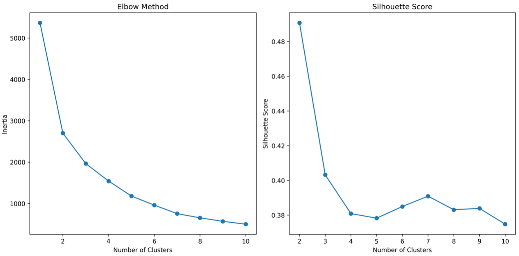
Elbow method (left) and silhouette score (right) for finding the optimal number of clusters for the (Bayesian Gaussian Mixture Model) BGMM clustering method.
Weekends, holidays and other untypical days are considered as days that have long-term planned incidents, when less travel demand might be seen during these days. Typical days, which mainly consist of weekdays, are used for the next steps in the framework. Approximately two thirds of the year are grouped as typical days in this stage. To assess the effectiveness of the clustering method in identifying untypical and typical days, the data were integrated with a calendar. Subsequently, a confusion matrix was generated, shedding light on the correlation between untypical days and weekends/holidays, as well as typical days and weekdays (Figure 7).
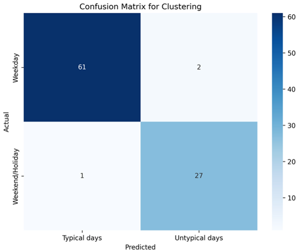
Confusion matrix for resulting clusters of (Bayesian Gaussian Mixture Model) BGMM clustering method.
Figure 8 illustrates the PCA scores plot after applying BGMM clustering.
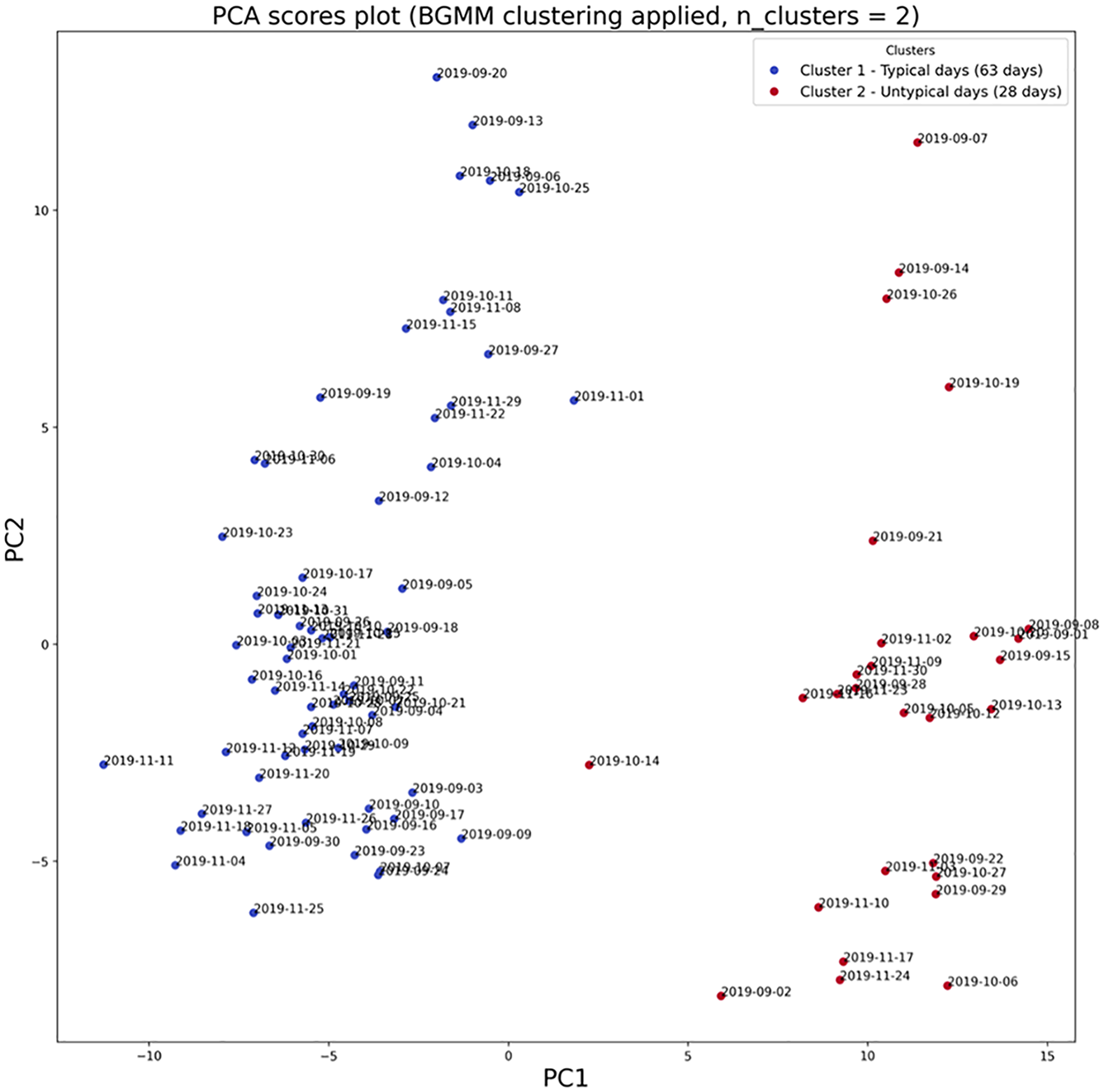
Principal component analysis (PCA) scores plot after applying (Bayesian Gaussian Mixture Model) BGMM clustering with n_cluster = 2.
Before getting to the next step in the framework, some features should be engineered for the purpose of this study. Because GTAModel is being run for the morning peak hour, the data used to build the VDF function should be consistent with this time frame. The data extracted from the StreetLight Data database are based on 15 min intervals. A rolling window of one hour is applied to the data. The number of observations in this window must be four. For each window, the speed is averaged and the traffic counts are summed. After applying the rolling window, a maximum of 93 pairs of 1 h-aggregated speed–flow pairs for each day are generated. After applying a 1-haggregation, the data are smoothed, accumulated, and less sparse, which facilitates the curve fitting. The 1 h-aggregated density (vpkpl) is calculated based on the speed, flow, and number of lanes (Equation 6). The lane-based density allows us to compare different road segments with different numbers of lanes.

where
After retrieving the typical days and appropriate features, we can continue to the second clustering stage. This clustering step aims to remove days with unusual traffic patterns. Weather conditions or other short-term unexpected incidents, for example, crashes, might produce this irregularity and between-day variability. The dissimilarity between the daily calibrated fundamental curves can be used to detect this issue and cluster the data to normal and abnormal traffic states. Therefore, before applying the clustering algorithm to the data, calibration of traffic flow fundamental equations should be done on a daily basis. For the daily calibration process, we selected the modified two-regime Greenshield model after evaluating various traffic flow fundamental models (refer to Figure 9). The decision was based on factors such as R-squared, root mean squared error (RMSE), and calibrated capacity, which align with the values specified in the HCM . The selected model consists of two parts: constant speed for the free-flow traffic condition and the modified Greenshield model for the congested traffic condition. As this model has a continuous form, it does not consider capacity drop, which helps to have less calibrated parameters to deal with in the next steps. The calibrated curve is drawn in Figure 9, and has the mathematical formulation as Equation 7:
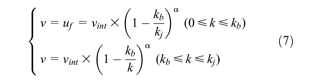
where
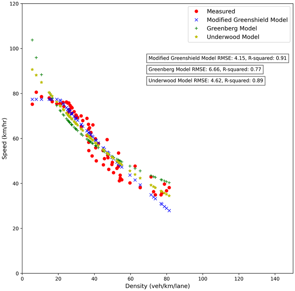
Modified two-regime Greenshield, Greenberg and Underwood traffic flow model calibrated with empirical data.
Among the three traffic fundamental equations, we have chosen the speed–density equation because it has a one-to-one mapping function which facilitates the calibration. The speed–density equation can be easily transformed into speed–flow and flow–density equations by using the fundamental traffic flow equation. The modified Greenshield model has four parameters that can be calibrated with empirical data. The jam density is considered to be constant and equal to 144 vpkpl, which is based on the assumption that the distance between vehicles in a traffic jam is 7 m. Therefore, free flow speed, breaking point density and power term are the three variables for calibration. For each day, the parameters of the speed–density equation are calibrated. The nonlinear least square method is used for the curve fitting procedure. The mathematical formulation of the least squares method (LSM) is expressed as Equation 8:

where
Parameter optimization setting
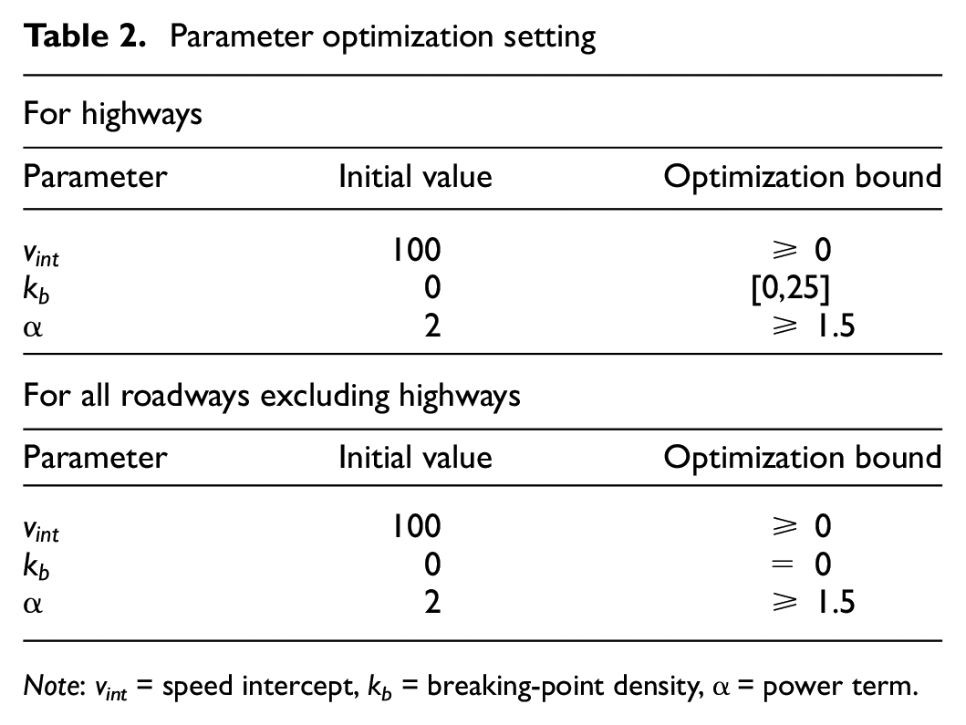
Note: vint = speed intercept, kb = breaking-point density, α = power term.
Following the calibration of each road segment, the R-squared and RMSE histograms are plotted and assessed across various dates for each road segment (Figure 10).
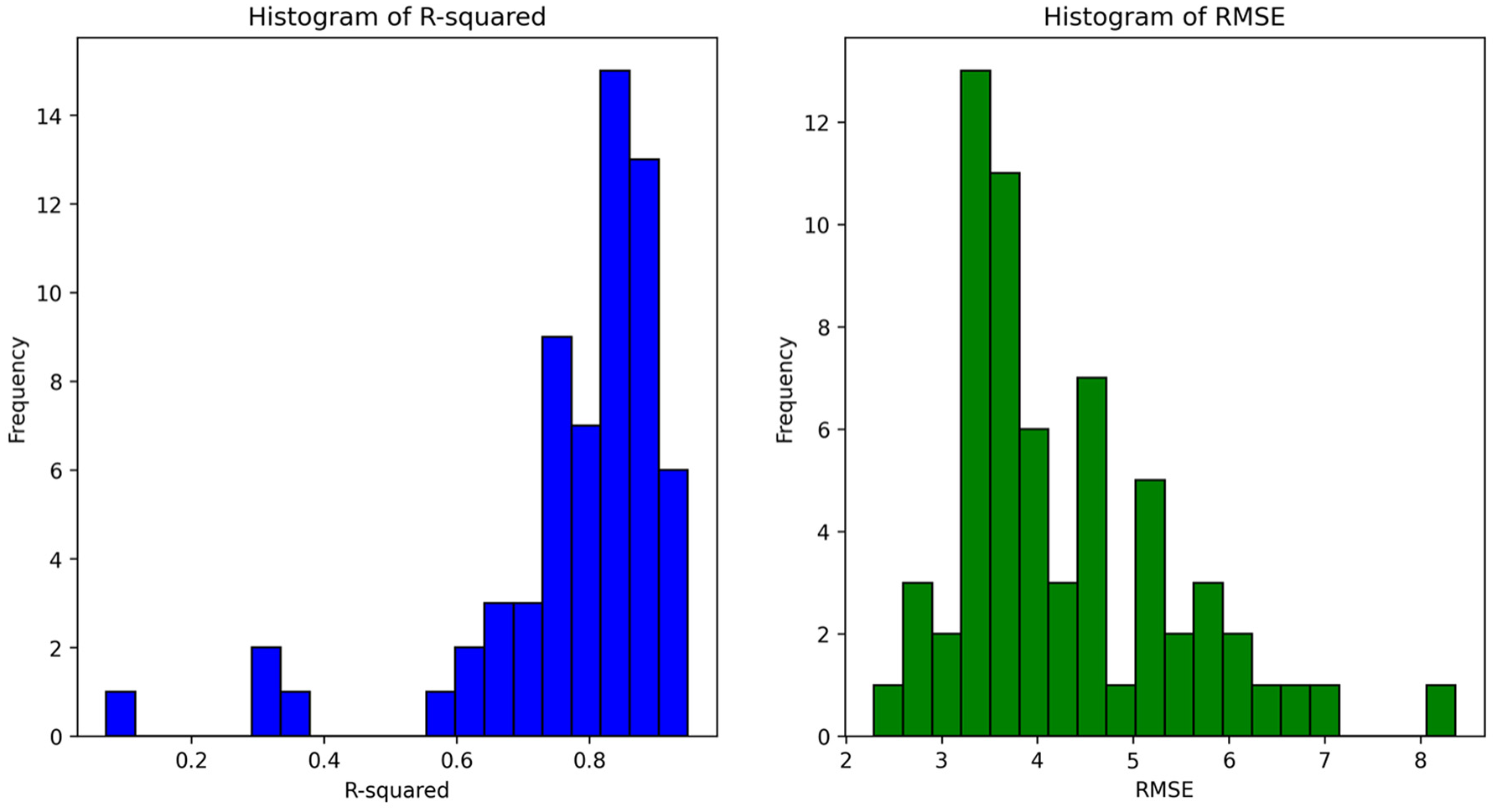
R-squared (left) and root mean squared error (RMSE) (right) histograms for a sampled road segment for different dates.
Since we calibrate on a daily basis and may not have enough data in the congested regime, the approach does not account for sample selection bias. At the end of the calibration process, we have a matrix with N*3 arrays, in which N is the number of rows (date of typical days) and columns are the three calibrated parameters. The clustering technique should be applied once the daily fundamental diagram calibration for the typical days has been completed. On the calibrated parameters, we have applied various connectivity-/centroid-/density-based clustering, and finally, hierarchical clustering with a modified affinity matrix is employed. The area between two calibrated curves is used as a measure of similarity between the traffic dynamics of different days. The area between curves is determined using 10 points from each daily calibrated curve to decrease computing costs. Other similarity measures can be employed to build the affinity matrix that is utilized in hierarchical clustering. In the modified hierarchical clustering approach, the optimal number of clusters is selected based on maximizing the silhouette score, as illustrated in Figure 11. Any clusters that have a sample size lower than three are eliminated, which are assumed as a cluster of abnormal traffic states.
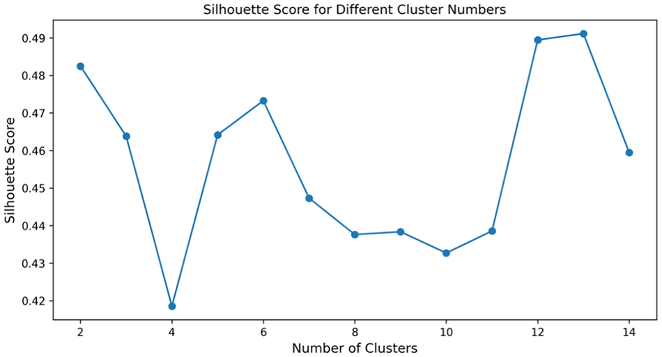
Silhouette score for different cluster numbers.
In this clustering stage, another between-day variability is captured, which is unexpected short-term incidents. Toward the end of this procedure, the cluster of typical days with normal traffic conditions is extracted, as shown in Figure 12. For this cluster, the mean values of calibrated parameters are calculated for being used in the last stage of clustering.
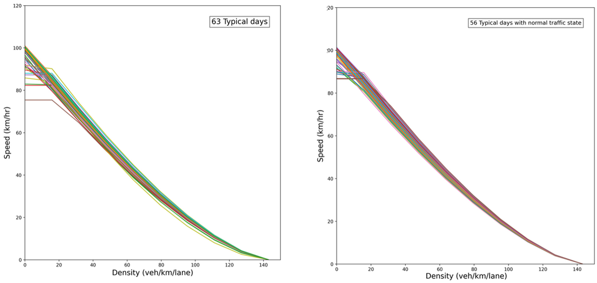
Daily calibrated speed–density diagram for one road segment before (left) and after (right) applying modified hierarchical clustering.
For each road segment, the first and second stages of clustering are conducted, and the mean calibrated curve is computed. By having one representative of each road segment’s traffic performance, the next step is to find the clusters of roadway functional classes. All road segments with their mean calibrated parameters are imported in the modified hierarchical clustering. The area between the calibrated curves of two road segments is the similarity measure in this clustering. The number of clusters is manually tuned depending on the user’s need and existing roadway classes manuals. Figure 13 depicts a speed–density diagram with clusters ranging from 3 to 8 after applying modified hierarchical clustering.
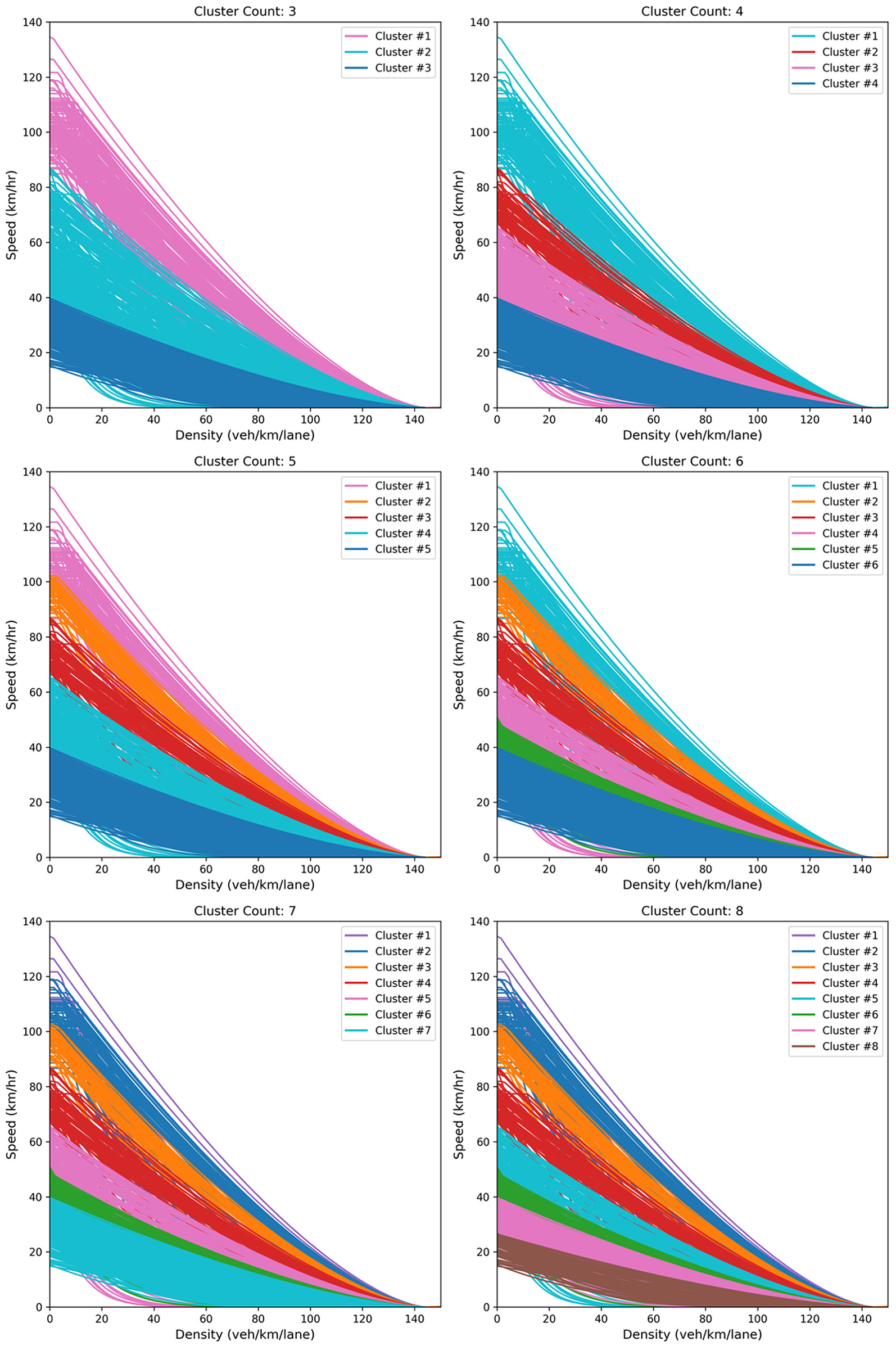
Speed–density diagram for all road segments after applying modified hierarchical clustering with n_cluster ranging from 3 to 8.
After finding the road functional classes, we should go through the last stage of the framework, which is VDF calibration. Data points for all road segments within one cluster are used for VDF calibration. Various VDF formulations are tested, and the one with the highest goodness of fit is chosen.
Results
In this chapter, we put our proposed framework into practice using observed data to assess the performance of the region’s various road functional classes. The calibrated parameters of the traffic flow fundamental diagram are shown. Using these calibrated diagrams as a basis, the free flow speed and capacity are computed and compared against the NCS16’s reported measures.
Daily Fundamental Diagram Calibration
In the second stage of clustering, daily fundamental diagram calibration is done. The R-squared value, a measure of goodness of fit, was found to be 0.76 on average for all calibrated road segments. The average RMSE of 6.3 (km/h) underscores the closeness of our predictions to actual values. Overall, our model demonstrates strong explanatory power in capturing the dynamics between speed and density.
Transitioning to the calibration results, the following section presents the existing and newly-calibrated free flow speed and capacity for all sampled road functional classes. As shown in Figure 14, the existing FFS in NCS16 for roadways in the City of Toronto’s downtown core is mostly 40–60 km/h, compared with GTHA borders which are mostly 70–90 km/h. Based on NCS16, highways have a free flow speed of 100–110 km/h. The calibrated FFS based on observed data has the same pattern as the NCS16 metrics.
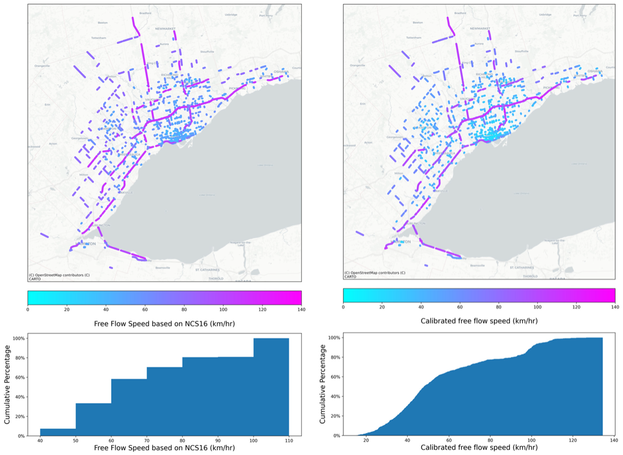
Spatial distribution (top) and cumulative percentage (bottom) of road segments with respect to free-flow speed (FFS) based on NCS16 (left) and calibrated data (right), for all volume-delay function (VDF) codes.
The reported capacity in NCS16 ranges from 400 to 2,000 vehicles per hour per lane (vphpl), although the calibrated capacity based on empirical data reveals another story. The calculated capacity ranges between 400 to 3,500 vphpl, where this upper bound exceeds the maximum reported capacities in previous works in literature (see Figure 15).
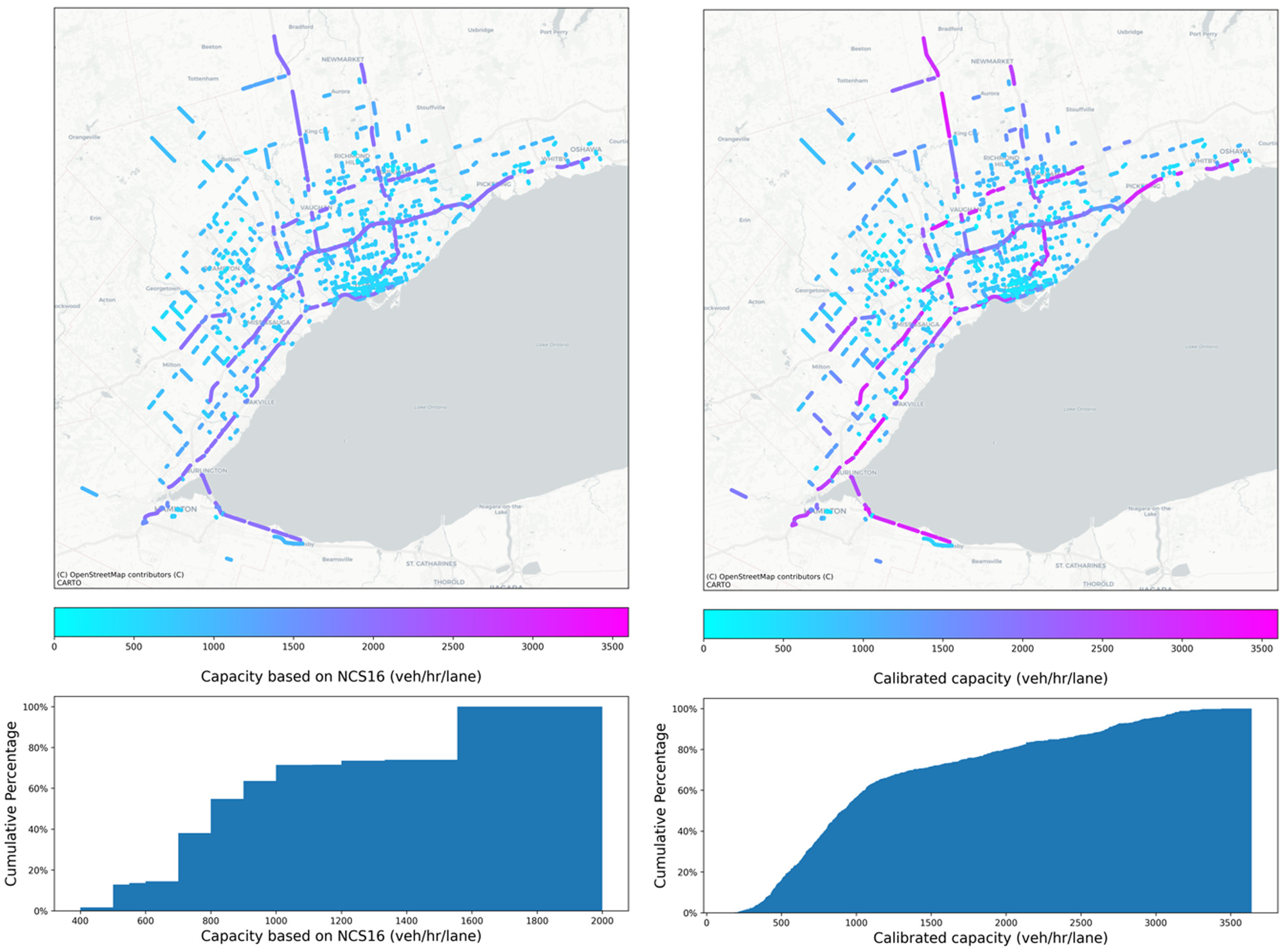
Spatial distribution (top) and cumulative percentage (bottom) of road segments with respect to capacity based on NCS16 (left) and calibrated data (right), for all volume-delay function (VDF) codes.
The difference between existing and calculated values of free flow speed and capacity is illustrated in Figure 16. This diagram shows that most free flow speed values in NCS16 are overestimated compared with reality. Furthermore, if we exclude highways, capacity values are well-estimated compared with NCS16. In regard to the highways, the capacity is underestimated in NCS16.
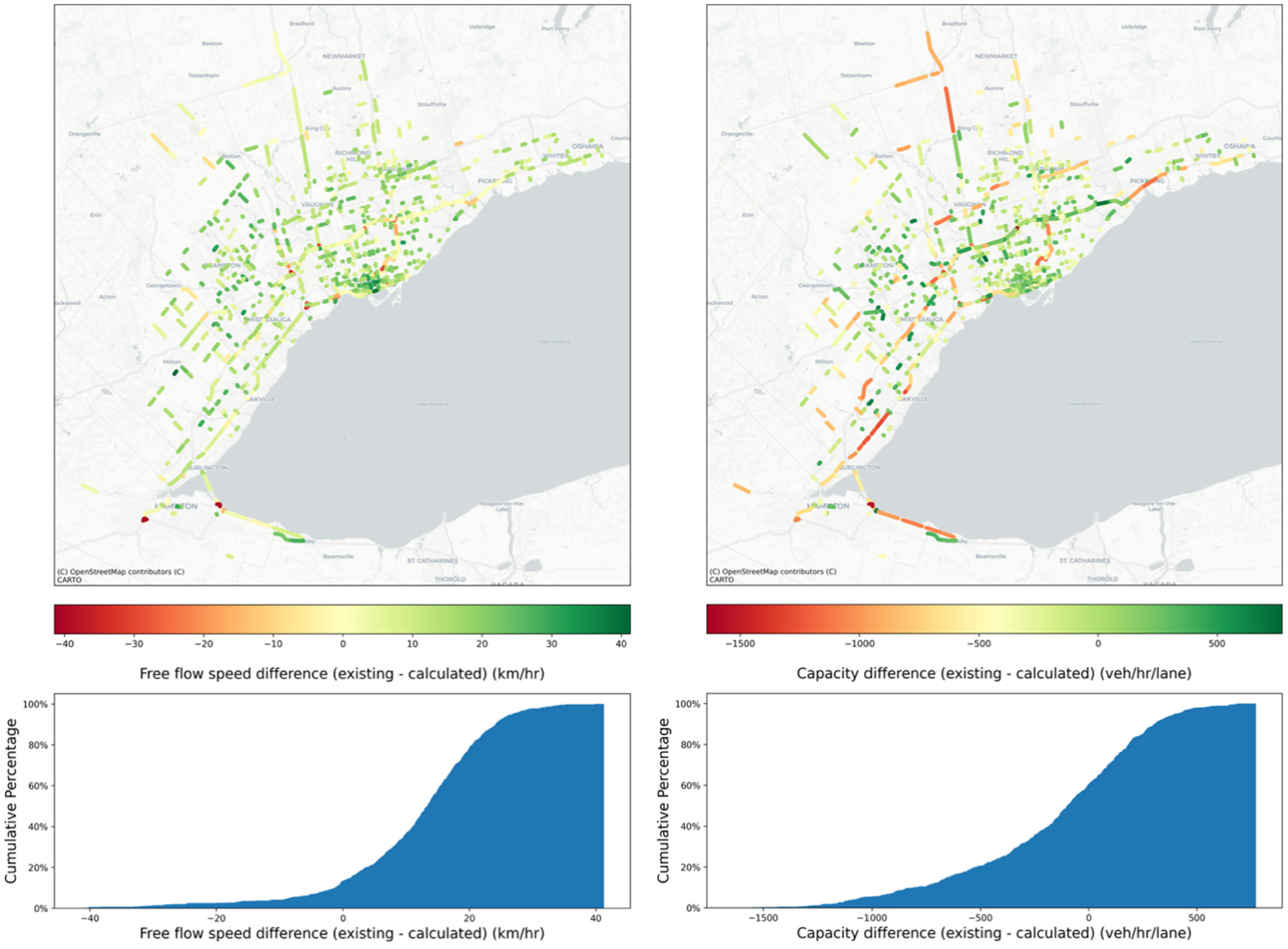
Spatial distribution (top) and cumulative percentage (bottom) of existing and calculated values difference of free flow speed (left) and capacity (right), for all volume-delay function (VDF) codes.
Figure 17 can help us compare the values of observed data with existing values in NCS16 in more detail. Roughly speaking, the data points are mostly close to the 45 degree line in both capacity and free flow speed curves. As can be seen by the fitted curve, most FFS data points are below the 45 degree line, which means the NCS16 is overestimating this metric. In regard to the capacity, if we exclude the high-capacity values, most of the capacity values are overestimated in NCS16. Real-world data show that for high-capacity values, which are mostly highways, NCS16 underestimates the capacity.
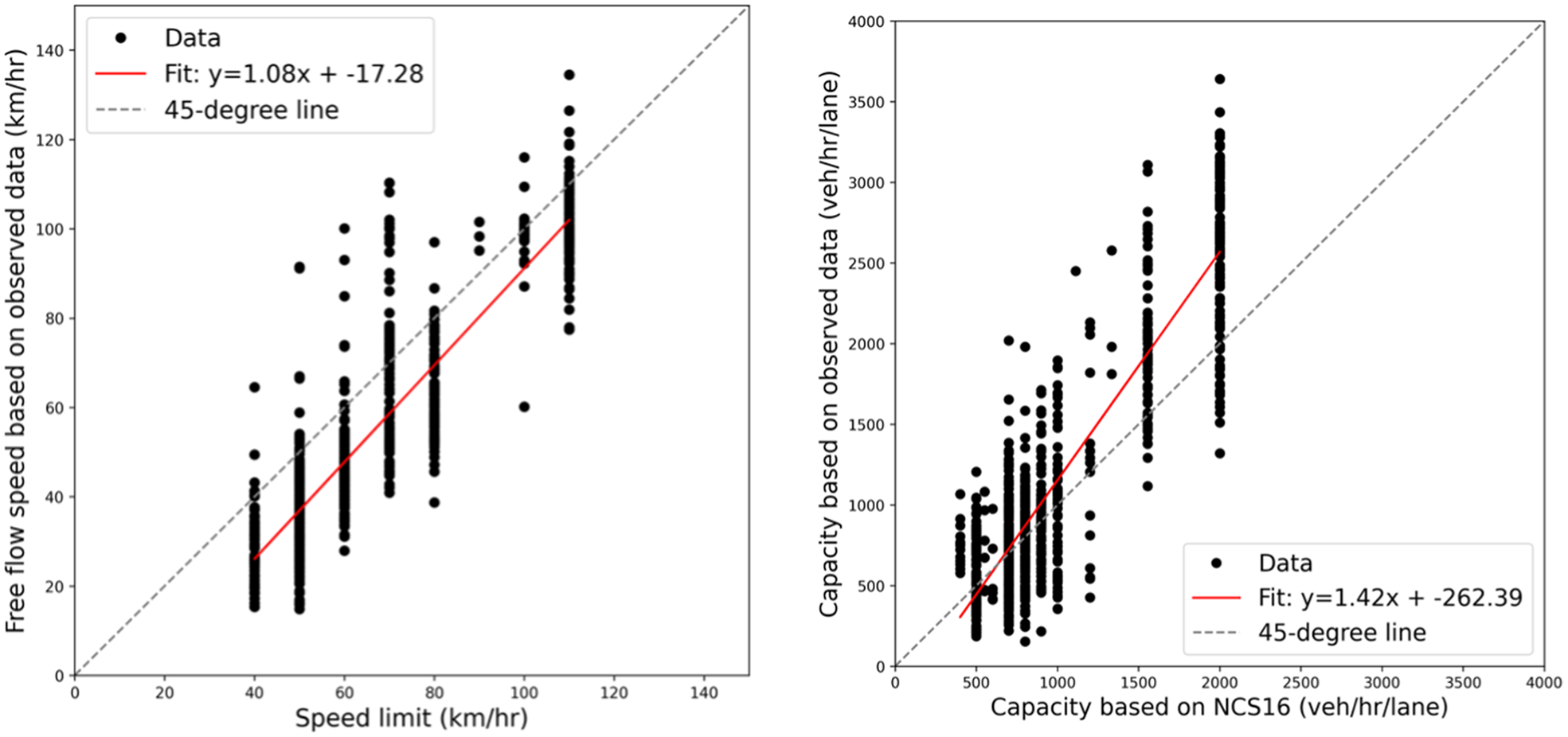
Comparison curve between existing and calibrated free flow speed (left) and capacity (right), for all volume-delay function (VDF) codes
Boxplots of Figure 18 demonstrate how free flow speed and capacity values vary over road segments with a similar number of lanes. Road segments with one or two lanes have lower values of free flow speed and capacity values compared with the road segments that have three or more lanes. Links with three lanes have the widest range of free flow speed and capacity compared with other links.
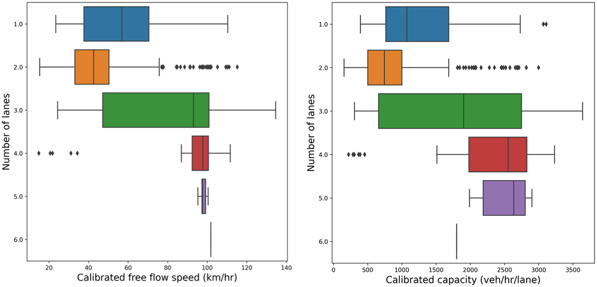
Box plot of calibrated free flow speed (left) and capacity (right) classified by the number of lanes, for all volume-delay function (VDF) codes.
Road Physical Attributes Distribution among Each Cluster
The traffic flow calibrated parameters are imported in the third stage of clustering, and new road functional classes are exported. After evaluating a range of cluster numbers, four clusters were used based on two principal considerations. First, ensuring that each cluster contained a sufficient number of roadway segments was critical for establishing statistical significance and robustness in the clustering results. Second, the selection of four clusters was intentionally made to enhance the clarity of visualization and interpretation concerning the distribution of land-use characteristics, lane numbers, and speed attributes within each cluster. This strategic choice facilitates a thorough and meaningful discussion of the clustering outcomes. Figure 19 shows the clustered road segments after applying modified hierarchical clustering, and Figure 20 demonstrates the spatial distribution of those segments. Clusters are named “Urban,”“Suburban,”“Rural,” and “Freeway.” As illustrated in Figure 20, the “Urban” cluster is primarily associated with the City of Toronto’s downtown core. “Suburban” and “Rural” clusters are mostly on the GTHA’s periphery. Highway segments are mostly found in the “Freeway” cluster. Figure 21 shows the distribution of the number of lanes within each cluster. The majority of the “Freeway” cluster is assigned to roadways with three or more lanes. In contrast, the major part of the “Rural” cluster is allocated to roadways with two or one lane(s). ‘Urban’ and ‘Suburban’ clusters are nearly identical concerning the proportion of lanes, with both having a great number of road segments with two lanes. “Freeway,”“Rural,”“Suburban,” and “Urban” clusters have the highest to the lowest proportion of higher-posted-speed road segments, respectively (Figure 22). The proportion of land use adjacent to the roadway is demonstrated in Figure 23. Land use near the roadway in the “Urban” and “Rural” clusters is mostly residential and open area, respectively.
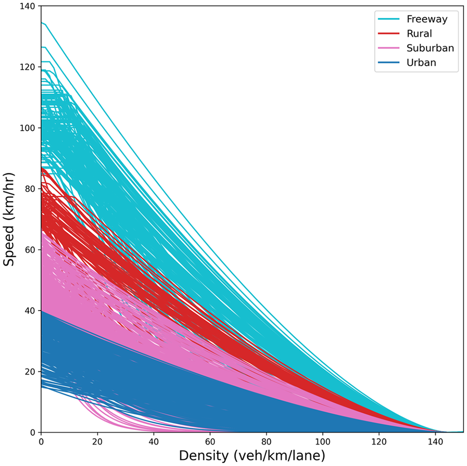
Traffic flow fundamental diagrams of all sampled road segments after applying modified hierarchical clustering with n_cluster = 4.
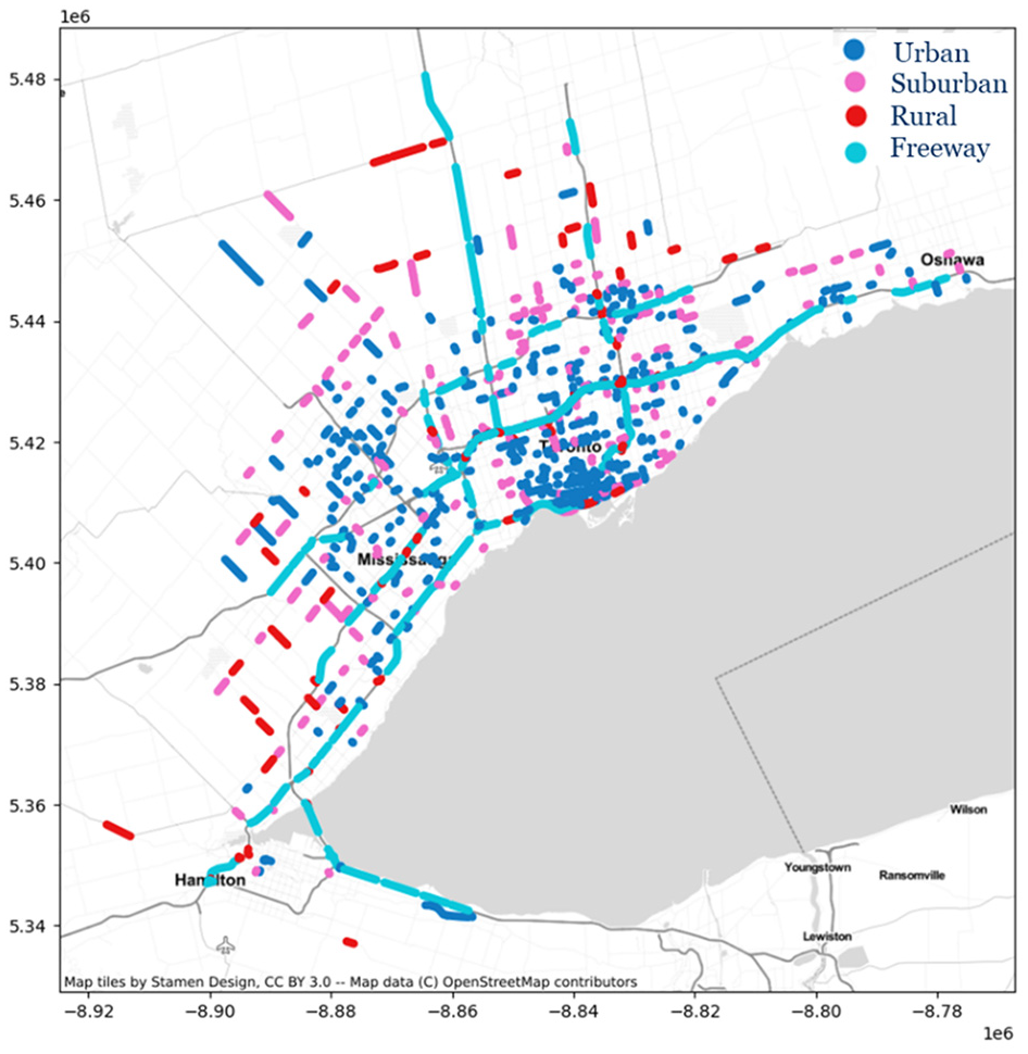
Clustered road segments, n_cluster = 4.
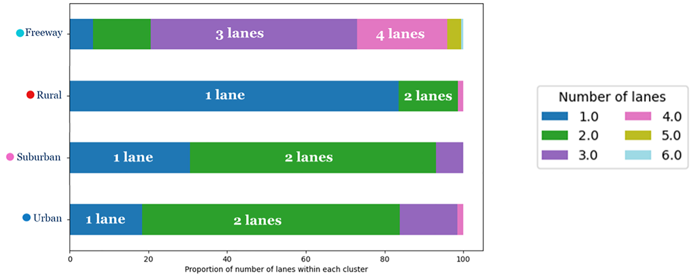
Distribution of “number of lanes” within each cluster.
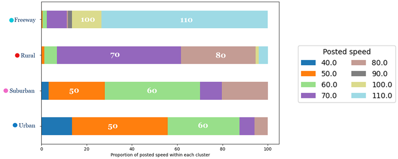
Distribution of posted speed within each cluster.
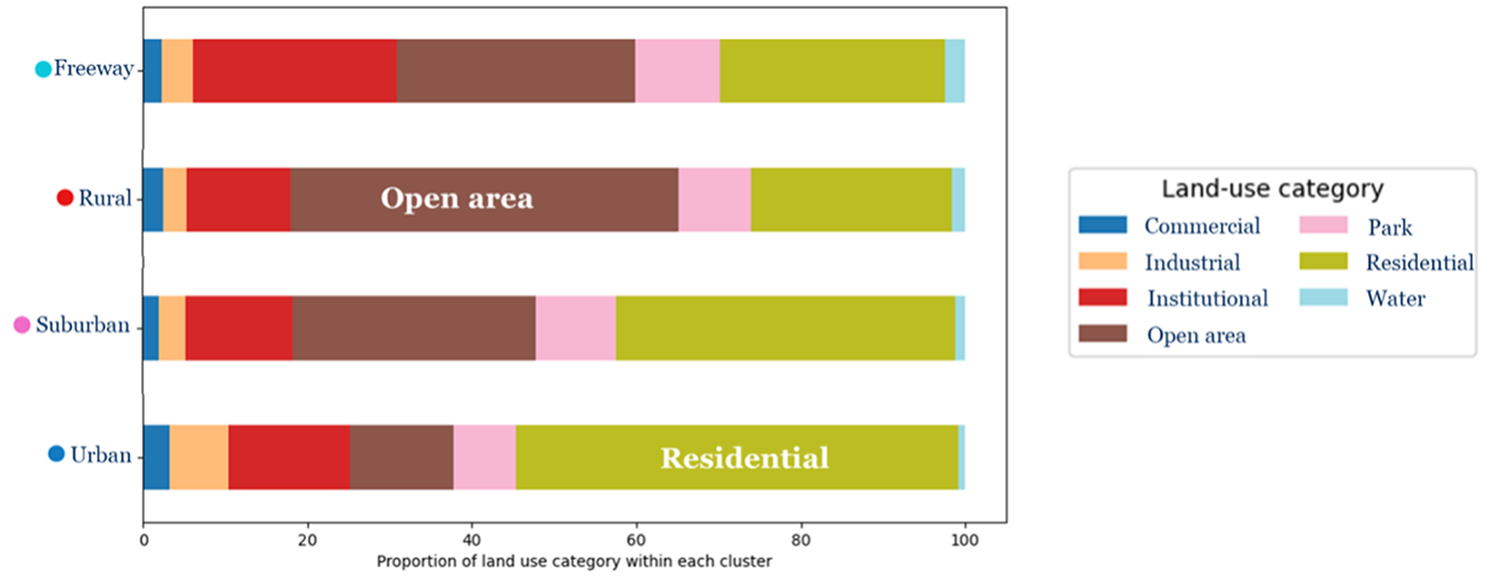
Distribution of land use category within each cluster.
Comparison of NCS16 and Proposed Road Functional Classes
To effectively compare our framework with the NCS16 classifications, we generated a Sankey diagram. This visualization is structured in two parts: one representing the primary grouping categories, and the other detailing the specific classes within the NCS16. Figure 24 displays the clustering of our framework alongside the high-level clusters in NCS16. It is evident from the diagram that our framework closely aligns with NCS16’s definition of Freeways. Additionally, our rural, suburban, and urban clusters map onto corresponding clusters in NCS16, although there are some discrepancies in full matching between these two manual/frameworks.
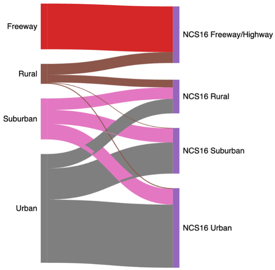
Distribution and alignment of clusters across NCS16 and our proposed framework.
In Figure 25, the left side represents the four clusters identified through our three-stage clustering approach, while the right side depicts the various VDF codes (12 classes) and their definitions according to NCS16. The diagram visualizes 27 flows between the nodes on both sides, offering insight into the distribution and alignment of clusters across both classifications.
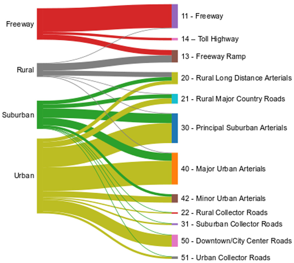
Detailed distribution and alignment of clusters across NCS16 and our proposed framework.
Conclusion
The current roadway network stands as the backbone of our mobility system, thus its preparedness to handle future challenges, emerging technologies and innovative solutions is critical. As we stand at the cusp of a transformative shift in transportation and urban development, our current understanding of what we possess is vital. This includes the performance of our existing roadways, an area that urgently warrants investigation.
Our research aimed to dissect and compare existing roadway performance metrics with those of a newly calibrated model, leveraging emerging data sources. This exercise gave us a realistic evaluation of infrastructural supply within static traffic assignments and enhanced our understanding of real-world, context-specific congestion behavior.
Our research significantly contributes to the field by introducing a novel approach to VDF classification and calibration. Unlike previous studies that have primarily focused on clustering various aspects of traffic metrics or individual speed–flow data points, our framework innovates by addressing how to define calibrated parameters for clusters comprising multiple road segments with varying road and traffic characteristics. This shift in perspective is crucial as it allows us to capture the nuanced behavior of road networks more accurately, considering the similarity between traffic and road characteristics of different segments. Our approach not only improves the accuracy of VDF calibration but also opens avenues for further advancements in modeling and simulation of traffic behaviors within complex urban environments.
We delved into the performance metrics of existing roadways in the GTHA’s NCS16, revealing an overestimation of the current FFS compared with the real-world calibrated data. The discrepancy seems to stem from the speed used in the GTAModel-based Emme traffic assignment, which is the posted speed and not always the observed FFS. Furthermore, our study indicated an underestimation of highway capacity in NCS16, despite non-highway segments being well-estimated.
We also examined the reliability of StreetLight Data, an innovative platform extracting traffic-related data from mobile crowd-sourced sensors. While the platform provides a unique opportunity to investigate any road segment or traffic analysis zone, we found that the metrics generated by StreetLight Data were not precise enough to model traffic behavior in all cases. Particularly, the volume estimates were not reliable for certain highway sections, despite the calibration options offered by the platform.
Our study highlights the limitations of the conventional roadway performance model used in static macroscopic traffic models. These models often fail to capture the dynamic nature of congestion, including queue accumulation and discharge, spillback, wave propagation, and capacity drop. In response, dynamic traffic assignment was proposed to capture these complex traffic behaviors. However, the implementation of a dynamic model for an entire city involves substantial data gathering, development, and calibration, making it a resource-intensive task, as well as being computationally very intensive.
Dynamic models, despite their high costs, are under development in several urban areas including the GTHA. The performance models in these dynamic models can be classified and calibrated using the framework developed in our study, albeit with a slightly different calibration process. However, it’s crucial to note that many other supply and demand characteristics also need calibration in dynamic models, a topic that was beyond the scope of our current study.
Future Research Opportunities
This research presents various opportunities for future studies, focusing on ten primary areas of exploration:
First, the research utilized processed location-based service (LBS) data, a novel source of big data emanating from GPS-fitted devices. The presented speed and flow metrics of this data source may not accurately reflect field traffic measures because of the reliance on GPS-powered probe vehicle data and machine learning techniques. Future studies could integrate loop detector data and Google Map application programming interface (API) or video-based measurements into the suggested framework to increase accuracy.
Second, the proposed framework’s spatial transferability is not region-specific, rendering it usable globally. Any traffic data source providing speed and volume values can operate the processing pipeline, assuming data availability and temporal resolution are adequate. More data over extended periods and finer temporal resolution may lead to better outcomes, given machine learning’s data-driven nature.
Third, while StreetLight Data, our study’s data source, provides road segment truck data, it is not an exact count but rather a depiction of relative truck activity. For a more comprehensive mixed traffic evaluation, researchers can scale up the relative truck activity data with ground-truth data for a region’s highways.
Fourth, the road segment sample selection in this study relies on a GTAModel-based Emme assignment run. However, alternative methods, like using Google Maps’ historical traffic data, could provide a more nuanced perspective of traffic congestion.
Fifth, calibrating the congested regime of VDFs using observed route choice data could help discern which VDF curves best replicate congestion patterns across the transport system. Two obstacles in using this data for this study involved StreetLight Data’s observed route discontinuities and the unreported routes between origin-destination pairs by the Emme static traffic assignment.
Sixth, this study did not consider the capacity drop phenomenon for calibrating the roadway fundamental diagram. Future research might employ a discontinuous two-regime traffic flow fundamental equation and a more thorough investigation of the jam density.
Seventh, as this study’s clustering framework employs a multistage unsupervised machine learning method, there is no performance assessment tool. Future research can use calendar and weather data to label unlabeled speed–flow data to evaluate the model’s accuracy in distinguishing holidays and weather events.
Eighth, the study invites sensitivity analysis tests on the model output based on input variables and parameter distributions. The technique could involve random resampling or Monte Carlo simulations to scrutinize several metrics like vehicle kilometers and average speed.
Ninth, the testing of different VDFs in EMME traffic assignment software and comparing the results with the Ontario Ministry of Transportation’s travel time studies may reveal useful insights.
Lastly, building on this study, future research could design macroscopic cost flow (MCF) functions to explore the network’s topological effect on traffic performance. By broadening the scope of the investigation, researchers will contribute to enhancing traffic data analysis, consequently improving road network management.
Footnotes
Author Contribution
The authors confirm their contribution to the paper as follows: Mohammad Amin Abedini: conceptualization, data analysis and modeling, writing – original draft, visualization, methodology, literature review; Eric J. Miller: supervision, review & editing, funding acquisition. All authors reviewed the results and approved the final version of the manuscript.
Declaration of Conflicting Interests
The authors declared no potential conflicts of interest with respect to the research, authorship, and/or publication of this article.
Funding
The authors disclosed receipt of the following financial support for the research, authorship, and/or publication of this article: The project was funded by NSERC (Natural Sciences and Engineering Research Council of Canada). Special appreciation to StreetLight Data for granting us their academic license, especially Peter Stokes and Antonio Gittens for their valuable support.