
Abstract
Traditional infrastructure funding sources have become insufficient because of increasing transportation demands and the impact of overweight (OW) vehicles, underscoring the need for a thorough evaluation of heavy traffic’s effects. This study presents a methodology to quantify the impact of OW vehicles on pavement performance and estimate the costs needed to offset their burden. The concept of the equivalent consumption factor (ECF) is introduced, and models are developed for various pavement structures and failure mechanisms. The analysis focuses on the Texas highway infrastructure system. Results indicate that the deterioration rate, represented by the power-law relationship between load ratio and damage, was lower for rigid pavements compared with asphalt concrete, except in cases of transverse cracking. For asphalt concrete, ECF values varied with the Structural Number when rutting was the primary failure mechanism. Flexible pavements generally required different ECF models, depending on axle configuration, whereas a single model sufficed for all rigid pavements. Using Texas’s low-bid unit prices, the cost per mile attributable to OW vehicles was calculated. Despite lower mileage, OW vehicles imposed per-mile costs at least 50% higher than commercial vehicles with greater mileage. The proposed methodology could potentially provide state highway agencies a tool to assess truck permit fees, enabling additional revenue generation and promoting sustainable infrastructure funding.
Historically, funding for the Texas state highway system has primarily relied on revenues from state and federal gas taxes. These funds are supplemented by various sources, including the State Highway Fund (SHF), Texas Mobility Fund, Proposition 1, Proposition 7, and the Build America Bond ( 1 ). Although these revenue streams have supported the development and maintenance of the highway system, they have faced growing challenges in keeping pace with the transportation demands of the state’s expanding population and their mobility needs. Moreover, alternatively fueled vehicles (that use sources of energy other than gasoline or diesel) have effectively reduced the total funds collected from the gas tax, which is the state’s most stable source of transportation revenue ( 2 ). In that context, it is imperative to evaluate the cost of constructing, maintaining, and rehabilitating transportation assets, such as pavements and bridges, to accurately gauge whether transportation revenues align with infrastructure needs and expenditures. This is not an easy task, as users do not consume pavement life equally.
Highways are used by a variety of vehicles, resulting in a wide range of possible axle configurations, loading levels, and tire sizes and leading to a complex deterioration process of the infrastructure system and, consequently, a complex cost allocation for maintenance and rehabilitation purposes as well. As expected, the structural life consumption of pavement and bridges is primarily attributed to trucks, including commercial vehicles (that adhere to federal weight limits) and overweight (OW) vehicles that are allowed to surpass weight limits in a controlled manner. These OW vehicles require special permits, issued from the Texas Department of Motor Vehicles (TxDMV), to operate within the Texas highway network. The revenue from these permits is then added to the state budget to address their incremental need of pavement maintenance and rehabilitation. However, adequately evaluating the effect of OW vehicles on pavement structures (and its associated costs) is a challenging task. Assessing the effect of heavy vehicles is also part of the risk management of the Transportation Asset Management Plan ( 2 ) that provides input to the Texas Department of Transportation (TxDOT) on permit fees and infrastructure affect costs of legal weight limits. Therefore, understanding how these OW trucks affect pavements and bridges is crucial not only for risk management purposes but also for helping state highway agencies (SHA) to adjust permit fees in a more equitable way.
The impact of OW vehicles on pavements is, and has been, the research object of many SHAs. A study conducted in Indiana showed that the pavement damage cost decreases drastically with the increase in the number of axles, for a given miles traveled, in a nonlinear fashion ( 3 ). The same study highlighted how aged infrastructures are less resilient, suggesting that aging should also be a factor to consider when routing heavy trucks permits. Middleton et al. ( 4 ) examined the challenges associated with identifying representative OW vehicles and determining their routes based on infrastructure structural capacity, as corridors for heavier trucks often do not align across states. The latest research study to evaluate the effect of OW vehicles with regard to pavement consumption was, in fact, conducted in Texas and is commonly referred to as the Rider 36 Study ( 5 ). This study, based on the work originally proposed by Prozzi and De Beer ( 6 ), introduced the concept of equivalent damage factors. The Rider 36 Study involved the quantification of the damage (and its associated costs) caused by OW trucks using the concept of structural life consumption. However, the study was restricted to sensitivity analysis over the possible axle load, since there was no available system at the time to aggregate the data on OW vehicles. Also, given the data availability, only two pavement types were considered based on their response behavior (rigid and flexible), without any further attempt to differentiate structure types.
This study introduces a comprehensive mechanistic-empirical modular approach, based on equivalent consumption factors (ECFs), to evaluate the effects of OW trucks on pavement performance across different axle configurations, pavement structures, and failure criteria. The proposed method aims to improve on the methodology developed in the Rider 36 Study, offering SHAs a rational framework to estimate the per-mile costs associated with OW loads. This approach supports the development of optimized permitting policies and contributes to a more equitable transportation system. Additionally, such an informed pavement evaluation method could facilitate the optimization on pavement management strategies and aid in selecting improvement alternatives, especially for corridors with high heavy-vehicle demand.
Factors of Interest in Pavement Analyses
Pavement Performance
Before the AASHO Road Test ( 7 ), there was not a quantifiable concept of pavement performance to determine if a pavement was acceptable. In fact, the lack of a proper continuously quantifiable failure criteria became evident even during the WASHO Road Test ( 8 ). The pavement serviceability index (PSI) was the first pavement performance parameter, and it was developed during the AASHO Road Test ( 9 ). The PSI is an index based on the concept that highways are provided for the comfort of the traveling public, and they ought to be safe and smooth ( 10 ). This index relates the subjective opinion of users (i.e., how they perceive the highway conditions on a scale from 0 to 5), with characteristics that are measured objectively, such as the amount of pavement distresses. The subjective evaluation of pavements, made by a panel of transportation-related individuals, called the present serviceability rating, was then correlated with the pavement evaluation performed during the road test. The findings showed that the unevenness of a pavement surface profile accounted for approximately 95% of the correlation coefficients in the PSI equation ( 9 ). Although pavement unevenness characterizes not distress itself but rather a distortion of the pavement surface, it was proven to contribute to an undesirable (or uncomfortable) ride. The results from the AASHO Road Test became the foundation for the AASHTO Guide for Design of Pavement Structures ( 11 ), which uses PSI as the performance measure.
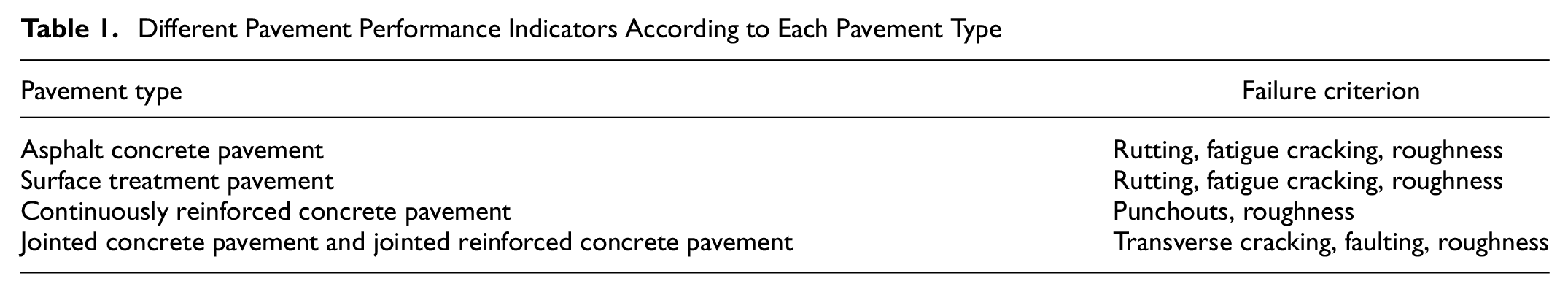
Many procedures are available for pavement design today, including those based on pavement mechanics, generally referred to as mechanistic-empirical methods. The attractiveness of these mechanistic-empirical methods lies in their ability to analyze the structural responses of layered systems and relate them to pavement performance using experimentally calibrated transfer functions. Since different pavement structures respond differently to load and weathering, it is expected that they would require specific failure criteria, as summarized in Table 1. Therefore, mechanistic-empirical methods are more comprehensive in capturing the nuances between pavement performances and structural demands.
Different Pavement Performance Indicators According to Each Pavement Type
Traffic Loading
Traffic plays a pivotal role in determining pavement performance and is one of the primary factors influencing design methods, alongside soil, environmental, and climatic considerations. Texas complies with federal restrictions on truck weights and has set weight restrictions to commercial trucks, as detailed in Table 2.
Weight Restrictions for Regular Commercial Trucks on Texas Highways
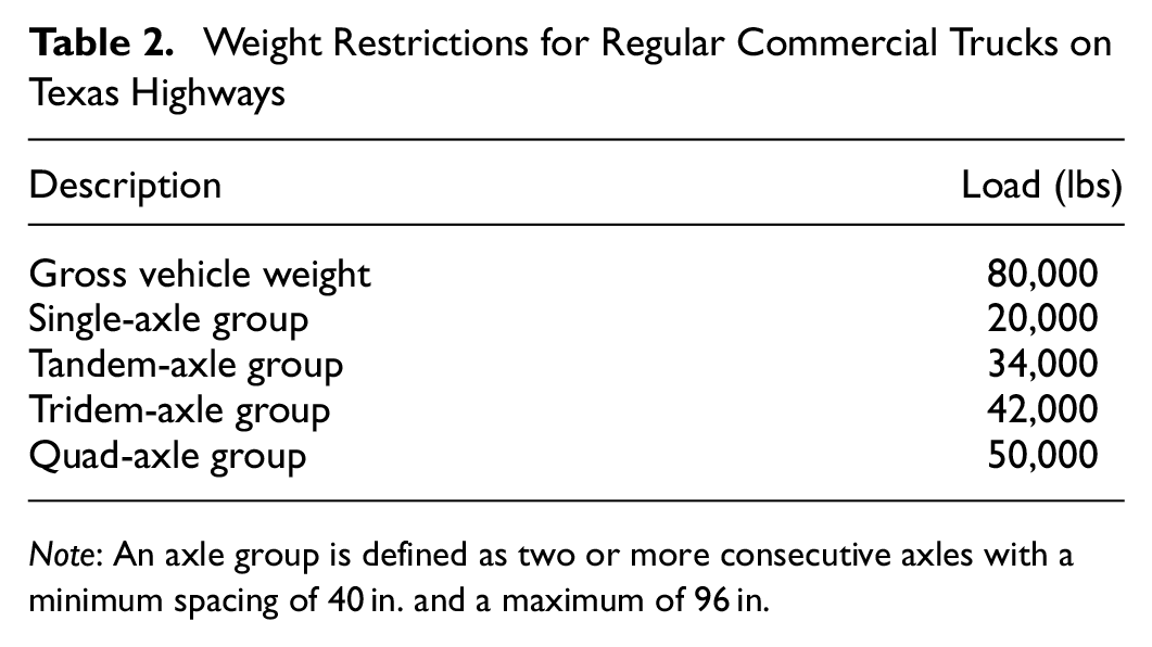
Note: An axle group is defined as two or more consecutive axles with a minimum spacing of 40 in. and a maximum of 96 in.
Motor carriers operating in Texas are also required to adhere to Federal Bridge Gross Weight Formula (FBGWF) weights. These weights were established by Congress in 1975 ( 12 ) and dictate the permissible weight-to-length ratio for a vehicle crossing a bridge to ensure structural integrity and safety. The FBGWF formula is shown in Equation 1:
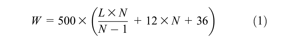
where W is the overall gross weight on any group of two or more consecutive axles to the nearest 500 lbs, L is the distance in feet between the outer axles of any group of two or more consecutive axles, and N is the number of axles in the group under consideration.
If a vehicle were to exceed the limits in Table 1, the motor carrier should apply for an OW permit at the TxDMV. The TxDMV processes approximately 800,000 oversize and OW permits every year. These vehicles can travel short distances of 10 miles or transverse the entire state using the state and county road network, but they cannot travel on the interstate system. The weight limit for permitted trucks is 650 lbs per inch of tire width or the axle-group limits shown in Table 3, whichever is lower.
Weight Restrictions for Carriers with a Permit on Texas Highways
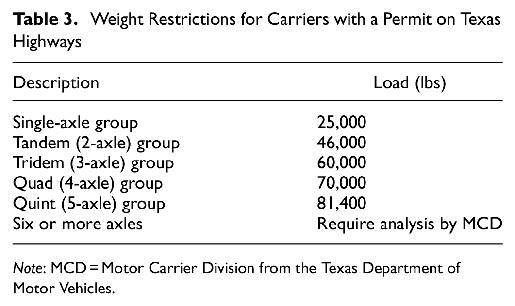
Note: MCD = Motor Carrier Division from the Texas Department of Motor Vehicles.
A web-based integrated geographic information system mapping, called the Texas Permitting and Routing Optimization System (TxPROS), is used in Texas for truck permit applications ( 4 ). This system provides automated routing for oversized and OW vehicles, categorizing them into one of 35 possible permit types, as defined by TxDMV. Of these, 16 are specifically related to OW vehicles. Table 4 presents a list of possible OW permits and each respective quantity issued from 2018 to 2022.
Number of Overweight Permits Issued Between 2018 and 2022 in Texas
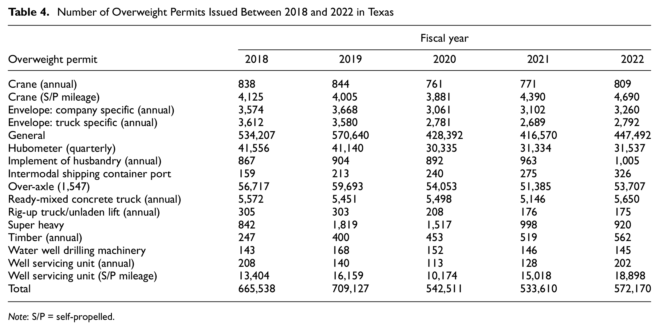
Note: S/P = self-propelled.
Table 4 shows a drastic change in OW permit demand between FY 2019 and 2020, as a result of the COVID-19 pandemic. This paper does not attempt to assess the relative impact on each permit type because of global crises. Instead, this analysis focuses on traffic patterns similar to those observed under typical conditions (e.g., 2019).
Climate and Environment
A pavement analysis must consider prevailing environmental conditions, which directly affect pavement performance. For example, rutting is more critical in warm climates, whereas cracking is the dominant distress mechanism in colder regions. Texas has five distinct environmental regions: wet-warm (Southeast Texas), dry-warm (South Texas), wet-cold (Northeast Texas), dry-cold (Northwest Texas), and mixed (Central Texas). In this study, the effect of the environment was captured by using pavement structures designed throughout the state of Texas (pooled from a library of projects obtained with the TxDOT), whereas climate was accounted for by selecting appropriate climate stations according to the pavement structure location under analysis. Statewide values were determined by averaging the results obtained from various state regions. This approach was necessary because of the lack of accurate routed data (i.e., origin and destination of the permitted trucks), which prevented a precise proportional assessment of regional effects on pavement performance.
Representative Pavement Structures
As mentioned, site features such as subgrade support and water-table level significantly affect pavement analysis. Therefore, a sample of 33 pavement design projects from various locations, built between 2017 and 2021, was drawn from the TxDOT project library for use in this study. Information such as layer thickness, elastic modulus, and traffic (with regard to equivalent single-axle loads [ESALs]) was essential to establish a comprehensive range of representative structures and traffic conditions found across Texas.
Economic Analysis
Highway costs are allocated to road users based on three key principles: marginality, completeness, and rationality. Marginality pertains to assigning costs to specific vehicle classes in a way that covers the expenses incurred by each class. Rationality ensures that the allocated costs for a vehicle class do not surpass what it would have paid in a smaller coalition or on a privately owned facility. Completeness involves recovering all highway expenditures by distributing costs among participating vehicle classes. Various methods exist for assigning highway construction costs to the appropriate entities ( 13 , 14 ), but in this study, a modified incremental method was utilized.
The regular incremental method involves constructing a pavement structure for the lightest vehicle class first and assigning the corresponding expenses to that group. This process is then repeated for progressively heavier vehicle classes, with pavement thickness and associated costs increasing accordingly for each category. However, the structural capacity of pavement increases exponentially with thickness, affecting how costs are distributed as heavier vehicles are added in sequence. Additionally, defining the lightest vehicle class can be subjective; a particular class may have a higher gross vehicle weight (GVW) but use more axles to distribute the load, which influences pavement distress differently. Pavement damage is affected by axle weights rather than just the overall vehicle weight.
Conversely, the modified incremental approach assigns highway costs to each individual vehicle category. After accounting for these costs, it then identifies and allocates highway expenses related to a coalition of multiple vehicle classes using a proportional measurement, such as their respective vehicle miles traveled (VMT). Accurate cost estimation using this method depends on adequate construction expenses estimates. In this study, this was obtained through TxDOT’s average low-bid price portal.
Pavement Consumption and Associated Costs
Pavement Consumption
The concept of the pavement ECF is based on that of the load equivalency factor (LEF) developed during the AASHO Road Test ( 7 ). The LEF represents the ratio between the repetitions of a given axle load and a standardized axle load (typically an 18-kip single axle). This equivalency provides a convenient way to index a wide range of possible axle loads to a single reference value: the standard axle. However, the LEF has limited applicability outside the specific conditions of the road test, especially concerning environmental factors, construction materials, and vehicle characteristics ( 15 ). Additionally, when the LEF was developed, more complex axle configurations (such as tridems and quads) and advances in tire technology (such as radial versus bias-ply tires) were not considered. Vehicle suspensions and tire pressures also differed significantly in the 1950s.
To address the limitations of the LEF, the ECF incorporates the effects of different pavement structures (pavement type and environment), climate, current axle groups (such as tridems and quads), and multiple failure criteria beyond those considered in the original road test. The ECF is similar to the LEF in that it relates the relative impact of an axle load to a reference load, ensuring they achieve the same level of performance. This relationship is known to be exponential, as is consistent with the linear approximation of elastic behavior in layered systems. Therefore, the ECF can be formulated as proposed in Equation 2, with its linearized form presented in Equation 3:


where Ni is the number of load repetitions of a given axle to reach a certain failure criterion; NS is the number of repetitions of the standard axle to reach the same failure criterion; Wi is the weight of a given axle of interest; WS is the weight of the standard axle (18-kip);
To associate all these factors involved in pavement analysis and obtain the respective number of ESALs, the AASHTOWare ME-Pavement Design was used. The AASHTOWare system computes pavement responses in a mechanistic-empirical analysis, assuming the pavement structure as a linear-elastic multilayered system. Although this is not the case, the linearity assumption is reasonable at the low strain levels typical of highway traffic ( 16 ). The critical pavement responses calculated by the software are correlated to field distresses using transfer functions, calibrated based on field observations, and using Miner’s law outputs the expected performance curves for the selected design life.
The basis for equivalency can be determined by either calculated (or measured) stress, strains, or deflections at various points in the pavement structure or by equal conditions of distress or loss of serviceability ( 10 ). Therefore, it is expected that the coefficient α (Equation 2), hereafter referred to as the axle load factor (ALF), is related to the pavement structure. This implies that different structures will be affected by axle loads at different rates, which is reasonable and consistent with observations made >70 years ago during the road test. A well-documented and established empirical index used to convert multiple pavement layers with different properties into a univariate is the Structural Number (SN). Although the SN does not fully account for the benefits of certain highway materials (e.g., inverted pavements, cement-treated layers, modified asphalt, etc.), it is still widely used by many SHA to characterize pavement structures.
The coefficient β (Equation 2) represents the effect of the axle group, hereafter referred to as the group equivalency factor (GEF), which would cause the same consumption (damage or performance) as a single-axle load. This is based on the axle configuration of the standard axle (18-kip single axle dual wheel). It is important to note that this coefficient addresses only the effect of different axle groups, using the number of axles (n) as a proxy for the variations in axle configurations.
Performance Criteria
To determine pavement performance over a specific period, a set of different failure criteria was defined for each pavement type from Table 1. The performance thresholds used, presented in Table 5, are the default values from the AASHTOWare design guide and are aligned with TxDOT’s requirements for pavement performance.
Failure Criteria Adopted per Pavement Type
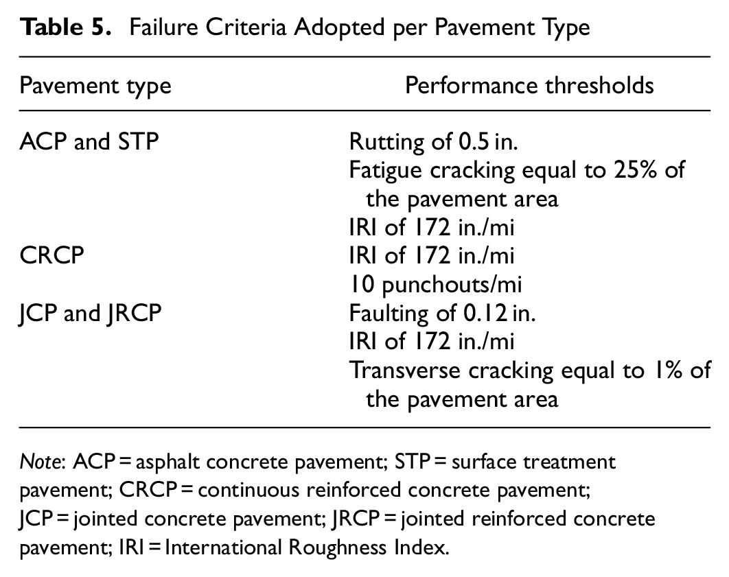
Note: ACP = asphalt concrete pavement; STP = surface treatment pavement; CRCP = continuous reinforced concrete pavement; JCP = jointed concrete pavement; JRCP = jointed reinforced concrete pavement; IRI = International Roughness Index.
VMT
The annual VMT for each OW permit was obtained directly from the routing reports through the TxPROS, when available, or estimated by meeting with TxDMV personnel who have been involved with OW permits for many years.
Calculating Consumption Costs
As mentioned earlier, this study adopted a modified proportional method for cost allocation. This was done based on the construction cost of an additional asphalt overlay to withstand the additional OW loads. In the case of asphalt concrete pavements (ACP), changes were performed by adding an asphalt overlay. In the case of rigid pavements, the concrete slab thickness was increased accordingly. This can be exemplified by assessing the effect of OW trucks on rutting performance, as shown in Figure 1.
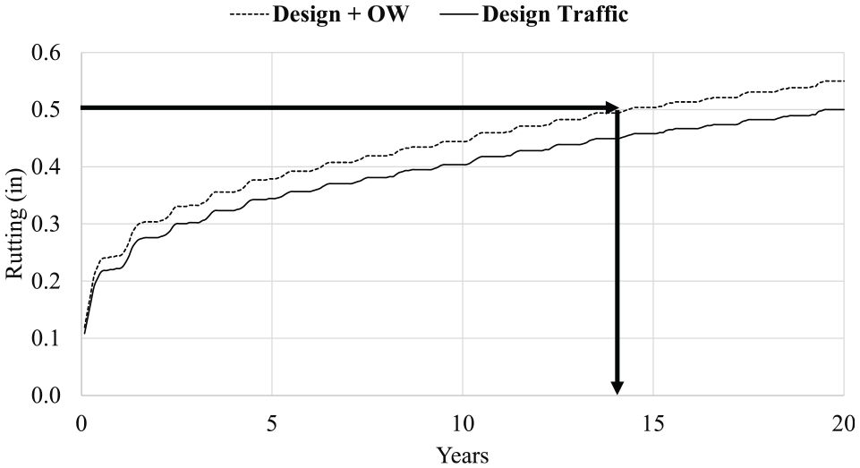
Effect of overweight (OW) trucks on rutting performance.
Notice that, in Figure 1, the pavement was designed for a certain traffic load (design traffic), assuming a 0.5 rutting performance threshold through the 20-year analysis period. Therefore, by adding the OW fleet, the pavement would experience a faster deterioration rate and an earlier failure. To account for effect of the OW fleet, the same pavement structure was redesigned with a new asphalt overlay of a given thickness. This adjustment ensures that the dashed curve (representing OW traffic plus design traffic) shifts toward the original continuous line, resulting in the same performance level as the original structure at the same intended 20-year period.
Results
This section presents the ECF models derived pavement analysis using the mechanistic-empirical approach proposed. To exemplify, a detailed description of the ECF model for rutting on the ACP is presented.
Traffic Load
Because of the nature of OW truck configurations, they may carry unconventional axle weights. Therefore, a comprehensive data exploration was conducted using the TxPROS database, and representative axle-load statistics were obtained, yielding the load spectra presented in Table 6. Since this study is part of a larger research effort aimed at updating truck permit fees in Texas, only the OW traffic data from 2019 were chosen to mitigate potential biases from the COVID-19 pandemic, thereby avoiding unreasonable policy adjustments that could negatively affect the state economy.
Axle Loads (lbs) Considered in the Analyses
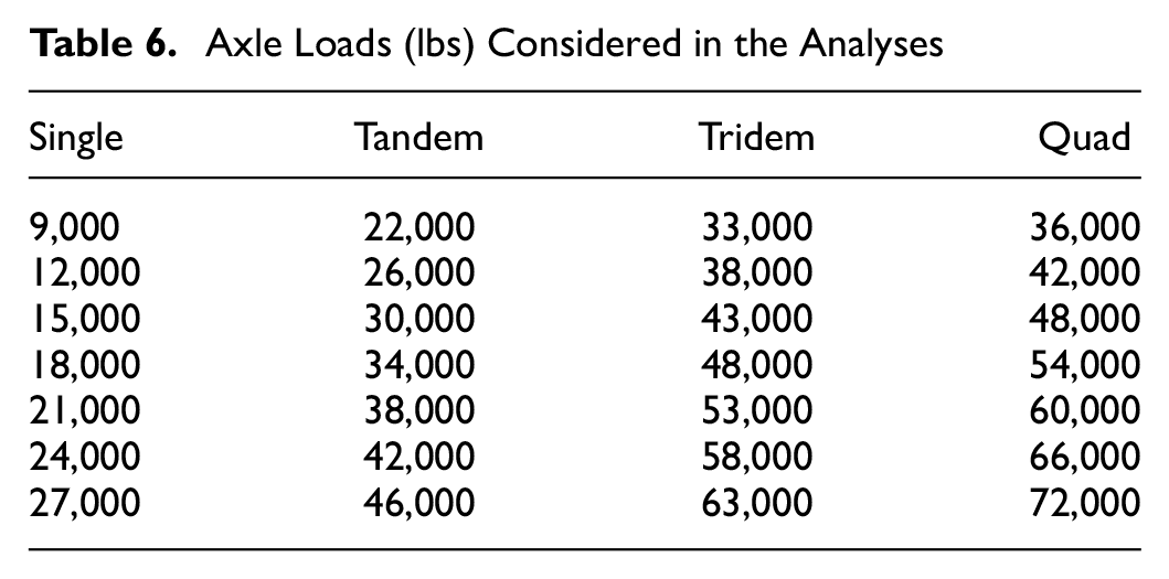
The axle-load intervals were constructed based not only on the data exploration but also by capturing important load values, including the standard axle (single axle with 18,000 lbs) and the maximum permitted weights for each axle group according to Texas legal limits: 25,000 lbs for single axles, 46,000 lbs for tandem axles, 60,000 lbs for tridem axles, and 70,000 lbs for quad axles. Axle groups with more than four axles were not evaluated because they were found not representative in the 2019 fleet.
Stepwise Process to ECF Modeling
The ECF modeling process is stepwise and somewhat iterative. Each pavement structure is analyzed multiple times, as there are 28 axle-load combinations and three pavement types, each with at least two failure criteria. The first step of the ECF modeling process is to evaluate the structural effect (α = ALF) for the various pavement structures. This step is crucial in analyzing how weaker and stronger structures, based on their SN, respond to different axle loads with regard to deterioration rates. The second step is to assess the group equivalent factor (β = GEF) by applying the 28 load combinations so that the pavement structure achieves the same performance as it would under the standard axle load (18-kip single axle). Here, the number of axles (n) serves as a proxy for the axle group, allowing the average GEF to be potentially estimated as a function of the axle count. The third and final step is to combine both the ALF and the GEF in either Equation 2 or Equation 3. If the coefficients for structure or axle groups yield approximate values, an averaged value may suffice instead of constructing a detailed relationship.
Since all variable relationships in the ECF model were developed on an ESAL basis, consumption cost estimates were calculated in dollars per ESAL mile. Specifically, the cost of the required asphalt is divided by the estimated VMT for each permit, yielding a unit cost per mile. It is important to note that the ECF relationships are valid only within the structure, axle load, and axle count parameters considered in the simulations, and extrapolation must be avoided.
ECF Model for Rutting on ACP
To obtain the linearized relationship between the ECF and the normalized log of load (Equation 3), different asphalt concrete structures were assessed, and the ALF (
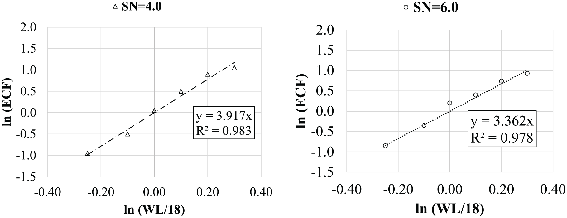
Axle load factor for two asphalt concrete pavement structures with different Structural Number (SN).
In principle, stronger pavements (greater SN) are less sensitive to load changes. Since another source of variability in the ALF could arise from the axle configuration, a sensitivity analysis for different level of SN and axle-group type was performed, as shown in Figure 3.
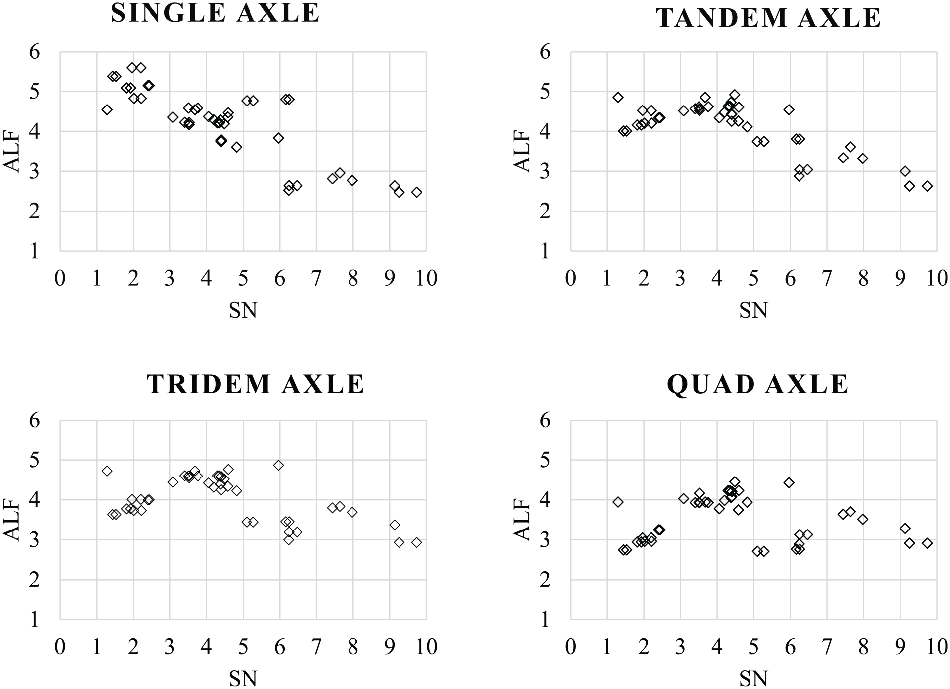
Effect of Stuctural Number (SN) per axle group on the axle load factor (ALF).
As it can be seen in Figure 3, the relationship between the ALF and the SN was found to be non-monotonic within the dataset considered. Further, the axle group with two or more axles appeared to have a “critical thickness” beyond which the ALF peaks and diminishes with increasing SN. Interestingly, the peak was common across the different axle groups at an SN equal to 4. In the case of single axles, it was noticed that by increasing the SN, there was a somewhat monotonic decreasing effect on the ALF. Based on this trend, two models were fitted: one for the monotonic case (single axles) and the other for the non-monotonic cases (the remaining axle groups) with a positively skewed asymmetry. Both ALF models suggested are presented in Equations 4 and 5, respectively:


where the subscript of the ALF indicates the number of axles and
Parameters for the Non-Monotonic Relationship (Equation 5) Between ALF and SN
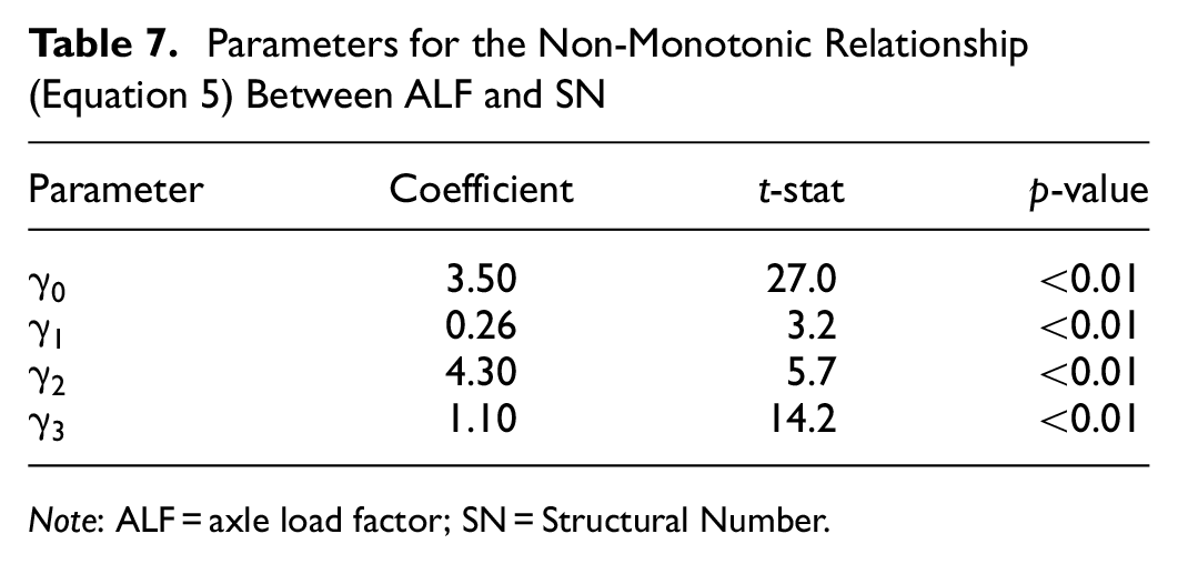
Note: ALF = axle load factor; SN = Structural Number.
Finally, the effect of axle groups that are not single axles was also quantified (
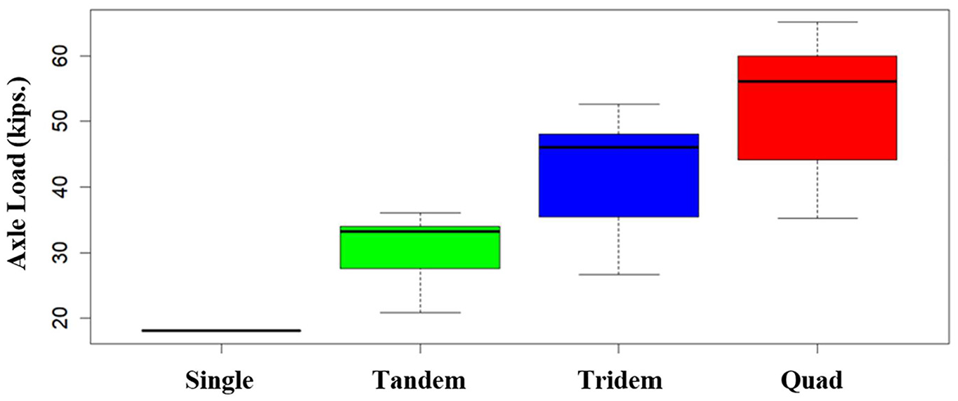
Axle-load variability to produce the same performance as the standard axle (18 kips).
For each axle group (tandem, tridem and quad), the ESALs that yield the same rutting performance as of the standard axle was obtained, allowing the calculation of the GEFs calculated. The GEFs were plotted against the number of axles (
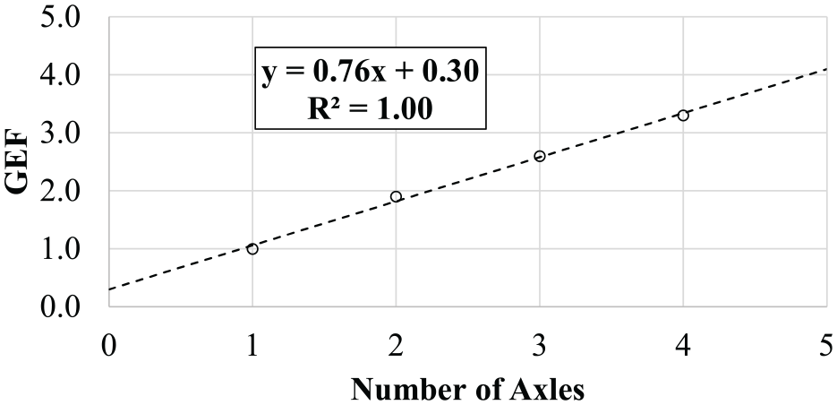
Linear relationship between the group equivalency factor (GEF) and the number of axles.
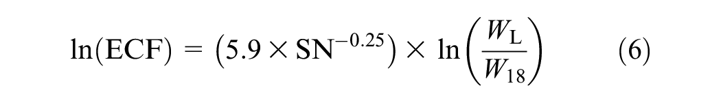
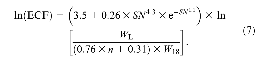
Combining all the results for the ALF and the GEF, the ECF model for rutting in the asphalt concrete for a single axle is shown in Equation 6, followed by a ECF model for the other axle groups other than the single axle in Equation 7:
The same procedure was repeated for the other pavement structures, axle configurations, and failure criteria. A list summarizing all the ECF models estimated is presented in Table 8.
Summary of the Mechanistic-Empirical ECF Models
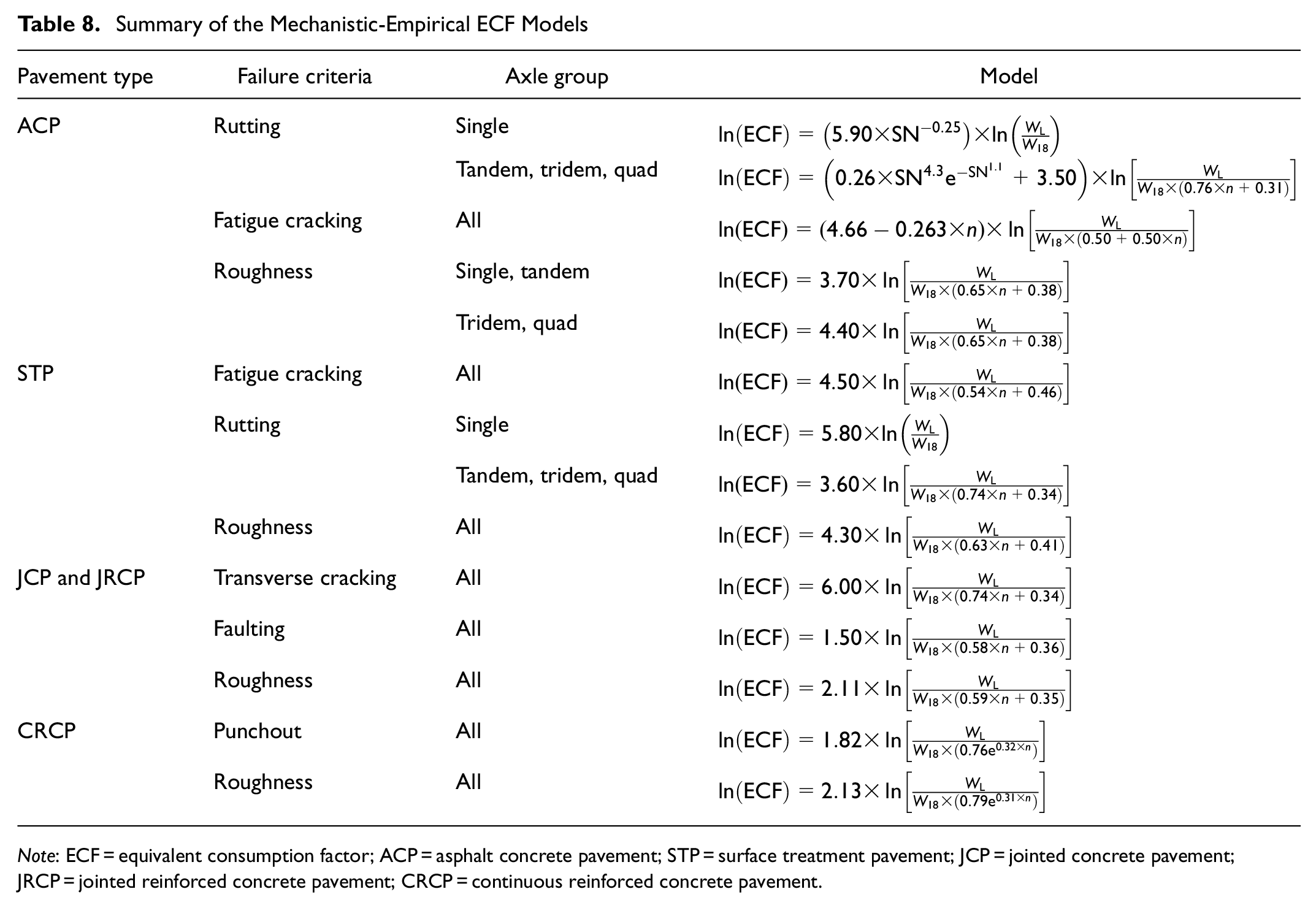
Note: ECF = equivalent consumption factor; ACP = asphalt concrete pavement; STP = surface treatment pavement; JCP = jointed concrete pavement; JRCP = jointed reinforced concrete pavement; CRCP = continuous reinforced concrete pavement.
Estimating Associated Cost
Among all OW permits of interest in Table 4, four permit types accounted for the majority of the VMT: general, hubometer, company-specific envelope, and truck-specific envelope. An estimated split of pavement types was used based on the proportions of each type of pavement in Texas. The general permits were further subdivided by GVW into four categories, and the Hubometer permits into two categories, resulting in a total of eight representative OW configurations. The pavement consumption costs for these configurations were calculated and are presented in Table 9.
Unit Consumption Cost Because of Overweighted Trucks
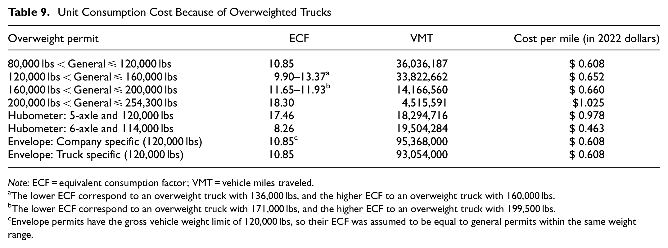
Note: ECF = equivalent consumption factor; VMT = vehicle miles traveled.
The lower ECF correspond to an overweight truck with 136,000 lbs, and the higher ECF to an overweight truck with 160,000 lbs.
The lower ECF correspond to an overweight truck with 171,000 lbs, and the higher ECF to an overweight truck with 199,500 lbs.
Envelope permits have the gross vehicle weight limit of 120,000 lbs, so their ECF was assumed to be equal to general permits within the same weight range.
The results indicate that approximately 57% of pavement consumption costs because of OW vehicles are caused by envelope permits, directly affected by the proportional VMT (60%) for the respective permits. Additionally, vehicles with greater GVW did not necessarily result in higher ECF, since the damage done to the pavement is related to the axle load instead. This explains the high ECF calculated for the hubometer permit with five axles and 120,000 lbs compared with the general permit within the same weight range. The cost-per-mile results from Table 9 indicate that, among OW trucks, particularly those with greater annual mileage, distributing loads across permits with lower ECFs can significantly reduce their cost per mile and consequently the permit fee. The total annual pavement consumption cost associated with OW vehicles was $199,308,940.
Conclusion
This paper presents a proposed mechanistic-empirical modular approach to address the effect of OW trucks on pavement consumption in Texas. This approach uses the concept of the ECF for different pavement types, axle loads, failure criteria, and environmental conditions. Finally, by combining the ECFs for all OW vehicle categories, along with their respective vehicle miles traveled, an associated consumption cost was calculated. To avoid potential biases from the COVID-19 pandemic, the data (truck configurations and VMT) used for the analysis considered only 2019.
The ECF models were successfully tailored using the primary engineering factors considered in pavement design and in the context of Texas. In the flexible domain, for asphalt concrete considering rutting as the primary failure criteria, the results indicate an exponential relationship between the ALF and the SN, regardless of the axle group, whereas for fatigue cracking, a linear relationship was found between the ALF and the number of axles within each axle group. In all other analyses, no relationship was observed between the ALF and the SN (or slab thickness in the case of rigid pavements), leading to the use of an averaged ALF value across different axle-group results. The GEF was found to have a linear relationship with the number of axles across all pavement types and failure criteria, except for continuous reinforced concrete pavement (CRCP). In CRCP cases, both punchout and roughness failure criteria were better described by an exponential relationship between the GEF and the number of axles. Most of the ALF calculated for the rigid pavement were less than half of the ALF calculated for flexible pavements, except for jointed pavement analyzed with regard to transverse cracking, which resulted in the highest ALF value within this study. Thus, it became evident that the exponent of the power relationship between pavement damage and axle load is sensitive to the structural capacity.
The costs associated with OW traffic were calculated using average low-bid unit prices in Texas. Total VMT for the OW fleet was obtained through data exploration in the TxPROS, the platform used by motor carriers to issue permits. Eight of the most frequent OW permits were identified, and one representative vehicle was selected for each. Vehicles with higher ECF values, such as those using a general permit (weighing between 200,000 and 254,300 lbs) and those using a hubometer permit (weighing 120,000 lbs), were found to have relatively low VMT. However, their impact on pavements became significant when assessing the cost per mile, which was at least 50% higher than other truck configurations.
Finally, this study provided a methodology to enable SHAs to estimate the damage cause to pavement structures by the OW fleet while also evaluating their truck permitting policy through a rational method. Consequently, by ensuring that OW fees accurately represent the level of damage inflicted on the infrastructure, a more sustainable funding source can be achieved. Regularly updating OW permit-fee structures is essential, in particular because of higher inflation and constant revenues from fuel taxes.
Footnotes
Author Contributions
The authors confirm contribution to the paper as follows: study conception and design: Danilo K. N. Inoue, Christian A. Sabillon-Orellana, Jorge A. Prozzi; data collection: Christian A. Sabillon-Orellana, Jorge A. Prozzi; analysis and interpretation of results: Danilo K. N. Inoue, Christian A. Sabillon-Orellana, Jorge A. Prozzi; draft manuscript preparation: Danilo K. N. Inoue, Christian A. Sabillon-Orellana, Jorge A. Prozzi. All authors reviewed the results and approved the final version of the manuscript.
Declaration of Conflicting Interests
The author(s) declared no potential conflicts of interest with respect to the research, authorship, and/or publication of this article.
Funding
The author(s) disclosed receipt of the following financial support for the research, authorship, and/or publication of this article: This project was conducted with the cooperation and support of the Texas Department of Motor Vehicles (TxDMV) and the Texas Department of Transportation (TxDOT).