Sage Journals: Discover world-class research

Abstract

Bus delays significantly affect urban public transportation by reducing operational efficiency and incurring high costs. Understanding the causes of these delays is essential for developing targeted mitigation strategies. While traditional research focuses on correlation-based analysis, it often fails to uncover the underlying causal mechanisms. This study examines various causal graph discovery algorithms combined with structural equation models (SEMs) to infer the causal relationships among factors that affect bus delays. These algorithms generate causal graphs for bus delays, revealing the interrelations and impacts of various operational factors. SEM is used to quantify the causal effects. This study evaluates the performance of these algorithms from the perspectives of both the statistical data fitting and the causal relationships generated. A case study is conducted using General Transit Feed Specification (GTFS) data from frequent bus routes in Stockholm, Sweden. The validation results demonstrate the effectiveness of data-driven causal discovery models in identifying causal links, particularly when combined with domain knowledge. The empirical analysis shows the complexity of factors contributing to bus delays, emphasizing the necessity of integrating causality into bus delay analysis. For example, a high correlation between origin delay and bus arrival delay (coefficient = 0.63) does not indicate direct causation, and a strong causation between dwell time and arrival delay does not imply a higher correlation (coefficient = 0.12). Comparing variable importance with linear regression (LR) reveals notable differences; origin delay, which is often overlooked by previous studies, is significant in the causal graph model (standardized coefficient = 0.601) but ranks much lower in LR (standardized coefficient = 0.003). These insights underscore the importance of automated, data-driven causal discovery in enhancing decision-making processes and improving the efficiency and reliability of transit services.

Keywords

data and data science data mining public transportation operations transformative trends in transit data big data GTFS

Bus delays have emerged as a significant and pervasive concern within urban public transportation systems, leading to considerable operating costs and inefficiencies ( 1 ). These delays not only inconvenience passengers but also undermine the overall effectiveness and reliability of public transportation networks ( 2 ). Therefore, understanding the causes of bus delays is crucial for developing effective mitigation strategies and improving the overall performance of bus services. However, existing research has predominantly focused on employing regression models to analyze correlations between various factors ( 3 – 6 ). While these studies provide insights into associations, they fail to reveal underlying causal relationships. To address the mechanisms behind bus delays and propose targeted solutions, it is necessary to explore the causal relationships between the various factors influencing bus delays.

“Causality” refers to the relationship between cause and effect, where one event (the cause) brings about or influences another event (the effect) ( 7 ). It is the concept that one event or variable is responsible for producing a change or effect in another event or variable. Unlike correlations, causality implies a directional relationship, suggesting that changes in the cause precede or lead to changes in the effect. The discovery of causal relationships in bus delays is important for several reasons. Firstly, identifying causal relationships goes beyond mere correlations and provides a more reliable foundation for decision-making and policy planning. Moreover, causal discovery models enhance the interpretability of results and offer a deeper understanding of the causal links between factors and bus arrival delays. By employing these models, transportation planners and policymakers can develop targeted interventions to address bus delays, leading to more effective solutions.

The existing literature on bus delay analysis has predominantly focused on identifying correlations between various factors and bus delays. Models developed for this purpose range from linear regression (LR) and statistical models to machine-learning-based approaches ( 8 – 10 ). There are many factors that affect bus arrival delays, which can be divided into three categories:

Operational factors: The set of variables that captures both the scheduled and actual activities of a bus during its trip, including scheduled travel time, dwell time, preceding stop delays, and initial delays ( 9 , 11 , 12 ).

Planning variables: The variables that describe the bus route and stops, capturing the heterogeneity of bus traffic, including the number of signals, signal intersections, and bus reserved lanes ( 3 , 4 , 13 ).

External variables: These include mechanical issues, weather conditions, and disruptions such as local events, accidents, and incidents ( 5 , 14 , 15 ).

Among these factors, extensive literature highlights the significant role of operational factors, including scheduled travel time, preceding stop delays, dwell time, and initial delays, among others ( 16 – 18 ). Although machine-learning-based models, especially deep learning models, are highly valued for their effectiveness, they often operate as “black boxes,” making it difficult to interpret the underlying delay mechanisms. Moreover, it is important to recognize that these methods are still based on correlations and do not reveal causal relationships. Among the sources of correlations, only causal relationships are stable and interpretable. The two most common sources of bias—unmeasured confounding and selection bias—can also manifest as mathematical relationships or correlations, a situation known as “spurious correlation” ( 19 , 20 ). For example, delay data for two bus stops on different routes at a traffic light intersection show a positive correlation. However, a more likely explanation is that this relationship is spurious and a third confounding variable (i.e., traffic signal) causes delays at both stops.

Furthermore, from the model perspective, studies analyzing bus delays are based on statistical models (e.g., LR, ordinary least squares) that generally assume independent variables that are not highly correlated ( 3 , 4 , 13 ). This overlooks the potential interactions and interdependencies between different factors. However, in practice, the above assumption is often unrealistic, as the bus delay is usually determined by the direct or indirect interaction of multiple variables. For example, driver behavior and traffic congestion affect both current and preceding stop delays. Additionally, the delay of the previous bus may affect the dwell time, which indirectly affects the delay of the current stop. These interactions affect the performance of bus services, and ignoring these relationships may lead to biased results.

To bridge the existing research gaps, this study explores a novel causal-based modeling approach to model bus arrival delays from a causality perspective, driven purely by real-time bus operational data. Our aim is to gain a comprehensive understanding of the underlying mechanisms causing bus arrival delays. This approach goes beyond traditional correlation-based analyses and delves into the causal relationships among various factors. Specifically, this paper infers the causal relationships between variables using causal discovery algorithms. Then, the structural equation model (SEM) is used to measure the causal effects between the variables ( 21 ). Compared with other models, SEM handles diverse variable types, complex relationships, and non-normal data, thereby enhancing visualization and causal estimation ( 22 ). However, it is confirmatory rather than exploratory and requires predefined structural graphs ( 23 ). Therefore, by using causal graphs generated by causal discovery models as inputs, both methods benefit: causal discovery shapes SEM structure, and SEM quantifies causal effects, optimizing the strengths of each approach. Finally, evaluation metrics are applied to assess the models’ performance. Besides the goodness-of-fit (GoF) metric, machine learning-based metrics (e.g., error rate, precision, F1 score) are used to evaluate the models’ performance in inferring causal relationships. The main contributions are:

Uncovering the causal relationships among operation factors and constructing a causal graph to illustrate their interconnections and impact on bus arrival delays.

Exploring various causal discovery algorithms to evaluate their performance and identifying the optimal approach for analyzing bus arrival delays.

Conducting a case study for selected high-frequency bus routes in Stockholm, Sweden, to identify and measure significant causal links and discuss practical implications.

The rest of this paper is structured as follows: The Methodology section presents key concepts, causal discovery algorithms, and the variables used in this study. The Case Study section describes the data, identifies causal factors, presents the results, and compares them with Pearson correlation and LR. The Discussion section explores the potential value of the causal discovery methods. Finally, the Conclusion section summarizes the main findings, limitations, and future research directions.

Methodology

Figure 1 presents the framework for analyzing various causal discovery models. The first step involves preparing the input data, which includes collecting bus arrival delay data, selecting operational variables, and incorporating domain knowledge to enhance the causal discovery models. The domain knowledge represents the general knowledge prevalent in public transport, which is distinct from the specialized expert knowledge in a highly specific area. A detailed explanation can be found in the Domain Knowledge subsection. The input data is then applied to the causal discovery model to infer causal relationships and generate causal graphs, which are subsequently fed into the SEM to quantify causal effects. Additionally, evaluation indicators are used to assess the models’ performance. Finally, the results are interpreted through examples. Cross-validation is conducted by comparing the importance ranking of variables to compare traditional correlation-based methods with causal-based methods.

Figure 1.

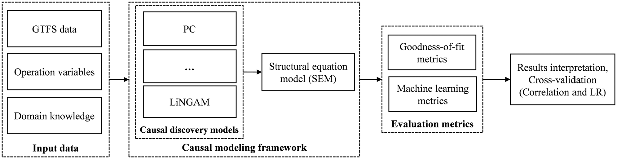
The framework for analyzing causal discovery models.

Causal Discovery Models

There are various causal discovery models for inferring causal relationships from observational data. We utilize a diverse set of algorithms to comprehensively analyze and evaluate their performance in inferring causal relationships in bus delays. Based on their operational principles, these algorithms can be divided into four categories: constrained-based, score-based, functional causal model (FCM)-based, and hybrid models ( 24 ). Below is an overview of algorithms selected for this study. Detailed model information can be referenced in the Appendix.

Constraint-Based Models

The constraint-based models conduct conditional independence (CI) testing between variables to check whether causality edges exist. These approaches deduce the CI within the data and search for a directed acyclic graph (DAG) that entails all (and only) these independencies according to the d-separation criterion ( 25 ). Numerous CI tests are employed, such as the conditional distance correlation test ( 26 ), momentary CI ( 27 ), and randomized CI test ( 28 ), among others ( 26 – 28 ). Typical algorithms include Peter-Clark (PC), conservative PC, and fast causal inference (FCI) ( 29 , 30 ).

Score-Based Models

The score-based models identify the most fitting causal graph by searching over the space of all possible DAGs using a search strategy and evaluating them with a score function. A variety of score functions are employed including the Bayesian Information Criterion (BIC), Akaike Information Criterion (AIC), and Bayesian Dirichlet equivalence score ( 31 – 33 ). One of the classical models is the Fast Greedy Equivalence Search (FGES) ( 34 ).

FCM-Based Models

The FCM-based models infer the causal relationship between variables in a functional form. They represent the variable as a function of the direct causes and unmeasured noise ( 35 ). They can distinguish between different DAGs within the same equivalence class by imposing additional assumptions on data distributions or function classes. One of typical model is the Linear Non-Gaussian Acyclic Model (LiNGAM) ( 36 ).

Hybrid Models

The hybrid models combine various causal discovery methods, such as integrating the CI test (constraint-based models) with score functions (score-based models), to create a hybrid approach for causal discovery. They include greedy FCI (GFCI), Greedy Relations of Sparsest Permutation (GRaSP), GRaSP-FCI, and Fast Adjacency Skewness (FASK) ( 37 – 39 ).

Different causal discovery models can handle different types of variable (continuous or discrete) and relationships between variables (linear or nonlinear), and are based on different assumptions (detailed in the Appendix). The dataset discussed in the study is static observational data with neither interventional information nor time dependencies. Table 1 shows the summary of the explored algorithms.

Table 1.

Models Classified by Supported. and Unsupported Settings

Model	Continuous	Discrete	Non-linear	Assumptions
Model	Continuous	Discrete	Non-linear	Causal sufficiency	Causal faithfulness	Acyclicity	Hidden confounder
PC	✓	✓		✓	✓	✓
CPC	✓	✓		✓	✓	✓
FGES	✓	✓		✓		✓
FASK	✓			✓	✓	✓
GRaSP	✓	✓		✓	✓	✓
FCI	✓	✓			✓	✓	✓
GFCI	✓	✓			✓	✓	✓
GRaSP-FCI	✓	✓			✓	✓	✓
LiNGAM	✓				✓	✓

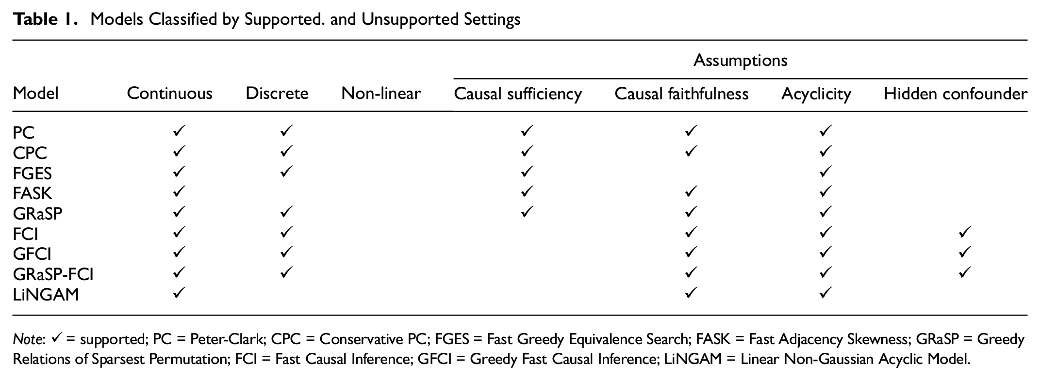
Note: ✓ = supported; PC = Peter-Clark; CPC = Conservative PC; FGES = Fast Greedy Equivalence Search; FASK = Fast Adjacency Skewness; GRaSP = Greedy Relations of Sparsest Permutation; FCI = Fast Causal Inference; GFCI = Greedy Fast Causal Inference; LiNGAM = Linear Non-Gaussian Acyclic Model.

Causal Modeling Framework for Factor Analysis

This study explores different causal discovery algorithms for bus arrival delay and evaluates their performance with and without incorporating domain knowledge. To quantify the causal effects between variables, we employ SEMs into the causal graphs generated from causal discovery models ( 40 ). The framework can also be found in a previous study ( 41 ). This framework not only identifies causal relationships and directions but also quantifies causal strength, thereby improving our understanding of the causal mechanisms driving bus delays. The evaluation framework comprises the following key steps:

Step 1: Generate causal graphs for bus arrival delays using purely causal discovery models.

Step 2: Utilize SEM on causal graphs to estimate the causal effects between variables.

Step 3: Incorporate domain knowledge, then repeat Steps 1 and 2, then compare the model’s performance before and after incorporating domain knowledge.

Step 4: Analyze and interpret the final causal graph and results from the optimal model.

Step 2 aims to map the causal graphs to SEM to quantify the causal strength among variables. Initially, according to the structure of the causal graph, each variable in the causal graph can be expressed as a structural equation with its direct causes (parent variables), that is, $v_{i} = f (Pa (v_{i})) + E_{i}$ , where $Pa (v_{i})$ represents the parent variables of $v_{i}$ , and $E_{i}$ is the error term. Subsequently, the maximum likelihood is used to estimate the parameter (i.e., regression coefficient) between variables. However, some algorithms (e.g., FCI, GFCI, GRaSP-FCI) may yield undirected causal relationships (e.g., ↔, °→, and °−°), which indicates the potential presence of unmeasured confounders between the variables. Such relationships do not illustrate a clear causal relationship and are not considered when applying SEM.

Bus Operation Delay Modeling

This study focuses primarily on investigating the operation variables that cause bus arrival delays. The bus operational data utilized in this research was obtained from Trafiklab (https://www.trafiklab.se/), an open platform for innovation in Swedish public transport. The data is based on the General Transit Feed Specification (GTFS) real-time vehicle location-based arrival time updates, which provide the actual arrival and departure times of each operating vehicle along its route. This can capture any service delays during operation based on the latest arrival time of each vehicle at each stop.

Table 2 provides an overview of the response variable and explanatory variables, along with their definitions. The response variable is the bus arrival delays at each stop. The explanatory variables contain various aspects of bus operations and are all continuous variables. The “origin delay” variable captures the impact of the initial delay on the route, revealing how these delays propagate and affect the current stop. Additionally, the “previous bus delay” variable accounts for knock-on delays, considering the delays experienced by the preceding bus and their potential influence on the arrival time of the current bus.

Table 2.

Description of Variables

Variable	Notation	Description
Response variable
Arrival delays	$d_{i, j}$	The arrival delay of bus $j$ at stop $i$ ; that is, the difference between the actual arrival time $t_{i, j}^{a}$ and the scheduled arrival time $t_{i, j}^{s}$ of bus $j$ at stop $i$ .
Exploratory variables
Dwell time	${dw}_{i - 1, j}^{a}$	Actual dwell time at the consecutive preceding stop; that is, the difference between the actual departure time $t_{i - 1, j}^{d}$ and the actual arrival time $t_{i - 1, j}^{a}$ of bus $j$ at the consecutive preceding stop $i - 1$ .
Preceding section travel time	$r_{i - 1, j}^{a}$	Actual running time between stop $i - 2$ and $i - 1$ ; that is, the difference between the actual arrival time $t_{i - 1, j}^{a}$ at stop $i - 1$ and the actual departure time $t_{i - 2, j}^{d}$ at stop $i - 2$ .
Scheduled travel time	$r_{i - 1, j}^{s}$	Scheduled running time between stop $i - 1$ and $i$ ; that is, the difference between the scheduled arrival time ${\hat{t}}_{i, j}^{a}$ at stop $i$ and the scheduled departure time ${\hat{t}}_{i - 1, j}^{d}$ at station $i - 1$ .
Preceding stop delay	$d_{i - 1, j}$	Actual arrival delay of bus $j$ at preceding stops $i - 1$ ; that is, the difference between the actual arrival time $t_{i - 1, j}^{a}$ and scheduled arrival time $t_{i - 1, j}^{s}$ at preceding stop $i - 1$ .
Previous bus delay (knock-on delay)	$d_{i, j - 1}$	Actual arrival delay of the preceding bus $j - 1$ before bus $j$ at stop $i$ ; that is, the difference between the actual arrival time $t_{i, j - 1}^{a}$ and scheduled arrival time $t_{i, j - 1}^{a}$ of preceding bus $j - 1$ at stop $i$ .
Previous bus travel time	$r_{i, j - 1}^{a}$	Actual running time of the preceding bus $j - 1$ between stop $i - 1$ and $i$ . It provides an indicator of the current traffic conditions.
Recurrent delay (congestion)	$d_{i, j}^{r}$	Recurrent delay (congestion) is trip-based; that is, the historical 1-month mean for the travel time of bus $j$ at stop $i$ during the same hour on the same weekdays. It provides an indicator of regular route traffic conditions. It reflects within-hour variations in traffic conditions using historical travel time observations. The historical 1-month data was used to get this value.
Origin delay (initial delay)	$d_{1, j}$	Actual departure delay of bus $j$ at the first stop; that is, the difference between the actual departure time $t_{1, j}^{d}$ and the scheduled departure time $t_{1, j}^{s}$ .
Scheduled headway	${\hat{h}}_{i, j}^{s}$	The planned time interval between the arrival time of two consecutive buses $j - 1$ and $j$ at stop $i$ .
Section length	$l_{i}$	The distance between stop $i - 1$ and $i$ .

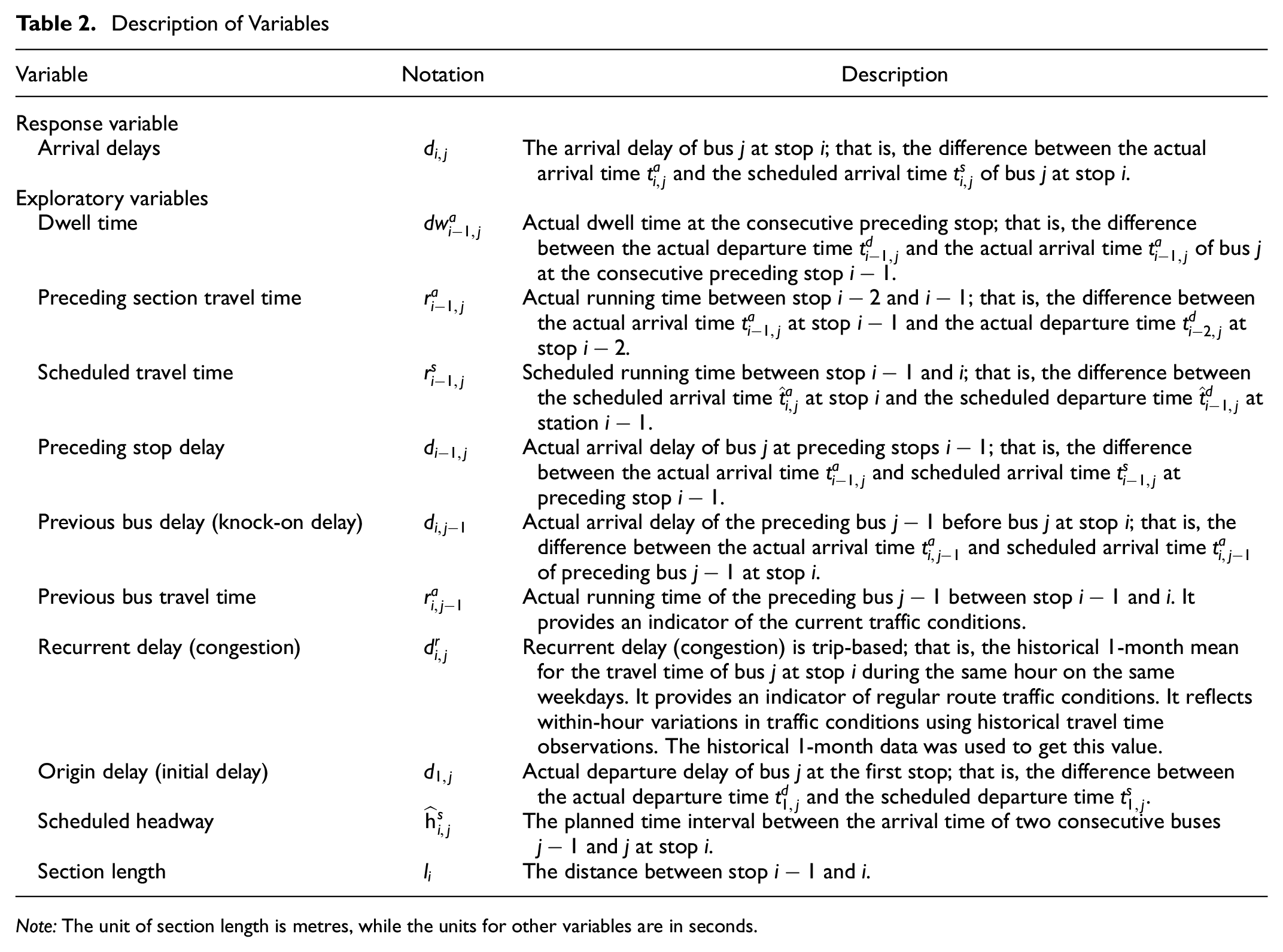
Note: The unit of section length is metres, while the units for other variables are in seconds.

Case Study

Data Preparation

The trunk line network of Stockholm was selected as the case study network. Figure 2 shows the four bus lines that form the core of Stockholm’s inner-city bus network. These four routes, encompassing over 200 stops and spanning 80 km, compose the backbone of Stockholm’s inner-city bus network, characterized by high-frequency services, designated lanes on main streets, traffic signal priority, and real-time information displays at all stops. Each route contains two to four public transport transfer stops. Moreover, these lines represent 60% of the area’s total ridership, serving approximately 120,000 boarding passengers daily from 7:00 a.m. to 7:00 p.m. ( 42 ). These routes are representative of typical busy urban public transport patterns and provide a sufficient data sample to analyze the causal effects of operational factors on bus delays. For analysis purposes, we collected data on bus arrival delays for May, 2022, covering both weekends and weekdays. Specifically, data was gathered from 6:00 a.m to 10:00 p.m., covering the operational hours of the bus service.

Figure 2.

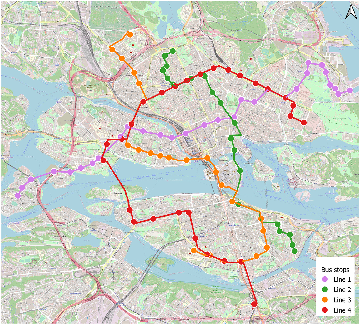
The inner-city bus line routes, Stockholm.

Evaluation Metrics

To evaluate the structure of the causal graph, it should be translated into SEM equations (a detailed description can be found in the Causal Modeling Framework for Factor Analysis subsection). The fit of the SEM model to the data is then assessed using GoF statistics, including root mean square error of approximation (RMSEA), comparative fit index (CFI), BIC, and chi-square (χ²) test ( 43 ). RMSEA evaluates the divergence between the model and the observed data per degree of freedom, with a lower value indicating a better fit. CFI measures the proportion of variance explained in the covariance matrix, with a higher value being preferable. BIC assesses the GoF of SEMs by balancing the model’s fit to the data and its complexity; a lower value suggests a better fit. The chi-square test reflects the model’s discrepancy, where a non-significant or lower value indicates a better model fit.

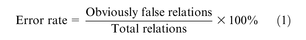
The above metrics aim to evaluate the causal structure generated by the algorithm from a GoF data perspective. To assess the overall performance, particularly the accuracy of the inferred causal relationships, several additional metrics are introduced: error rate, recall, precision, accuracy, and F1 score ( 44 ). The error rate, for example, represents the ratio of evidently false relationships (e.g., dwell time → preceding stop delay, dwell time → preceding section travel time) to the total number of relationships in the causal graph. The error rate of relationships can be expressed as follows:

Error rate = \frac{Obviously false relations}{Total relations} \times 100 %

(1)

In the context of a causal graph, the terms true positive (TP), true negative (TN), false positive (FP), and false negative (FN) are typically defined as follows:

TP denotes true edges that are present in the estimated causal graph.

TN denotes true edges that are absent in the estimated causal graph.

FP denotes false edges that are present in the estimated causal graph.

FN denotes false edges that are absent in the estimated causal graph.

Since there is no ground-truth causal graph or relationship available, and to ensure a fair comparison among different algorithms that generate varying numbers of edges, we established 10 obvious true relation assertions (true edges) and 10 obvious false relation assertions (false edges). This approach allows for a consistent baseline for evaluating the performance of the algorithms, enabling a meaningful comparison based on the same set of predetermined assertions. Table 3 displays the predetermined correct and false causal relationship assertions based on domain expert knowledge. These 20 assertions serve as the actual values, while the causal relationships in the estimated causal graphs represent the prediction values.

Table 3.

Correct and False Causal Relationship Assertions

True assertion	False assertion
Preceding stop delay → arrival delay	Dwell time → preceding stop delay
Dwell time → arrival delay	Dwell time → preceding section travel time
Scheduled travel time → arrival delay	Scheduled headway → dwell time
Scheduled travel time → previous bus delay	Section length → preceding section travel time
Preceding section travel time → preceding stop delay	Preceding stop delay → preceding section travel time
Previous bus travel time → previous bus delay	Previous bus delay → previous bus travel time
Recurrent delay → previous bus travel time	Preceding stop delay → previous bus delay
Origin delay → preceding stop delay	Scheduled travel time → preceding section travel time
Preceding section travel time → dwell time	Section length → origin delay
Section length → scheduled travel time	Origin delay → previous bus delay

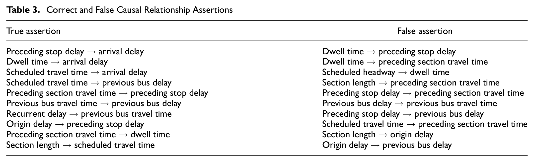
Establishing accurate assertions requires building on existing transportation literature. Previous studies support the view that factors such as preceding stop delay, dwell time, and scheduled travel time significantly contribute to bus arrival delays ( 14 , 45 ). Based on these insights, we confidently formulated some assertions about previous bus delays and preceding stop delays. Moreover, consultations with domain experts further validate these assertions, affirming the logical mechanisms through which one variable influences the other in the public transportation context. Additionally, comparative analyses are performed to ensure the plausibility of these relationships relative to other relationships.

Finally, the evaluation metrics used serve two main purposes: assessing data fit through GoF statistics (e.g., RMSEA, CFI, BIC) and evaluating relation generation via machine learning metrics (e.g., recall, precision, F1 score). Each category contains multiple indicators that examine different aspects, providing complementary insights into model performance. Relying on a single metric can give a skewed view, such as a model with high precision but low recall missing many TPs. Different applications may prioritize different metrics. Our paper aims for a comprehensive view of model performance, so using a broad set of metrics allows for thorough and accurate evaluation.

Domain Knowledge

As described in the framework shown in Figure 1, this study incorporates domain knowledge to enhance causal algorithms and compares the accuracy of causal inference obtained with purely data-driven methods. According to the order of occurrence, the variables are categorized into distinct tiers. Figure 3 shows the hierarchy of variables. Within this hierarchical framework, causal directions flow only from upper-tier variables to lower-tier variables; that is, the lower-tier variables cannot influence the higher-tier variables.

Figure 3.

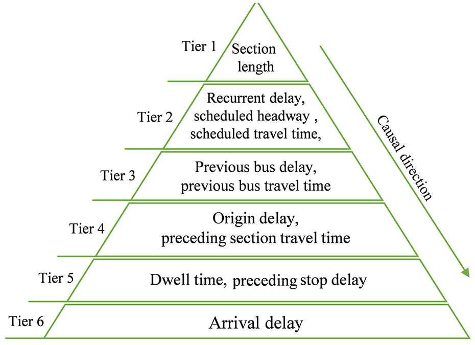
Hierarchical organization of variables.

Within the same tier, certain relationships are deemed forbidden because of the spatiotemporal occurrence order inherent in the public transportation system. Specifically, as far as spatial limitation is concerned, the scheduled variables of a current section do not affect the variables of the preceding sections. This implies that changes or variations in the scheduled parameters of the current section do not affect the corresponding variables in the preceding sections. The forbidden relationships are elucidated as follows:

1) Temporal occurrence order constraints: previous bus delays ↛ previous bus travel time; preceding section travel time ↛ origin delay; dwell time ↛ preceding stop delay

2) Spatial occurrence order limitations: {scheduled travel time, scheduled headway, and section length} ↛ {preceding stop delay, preceding section travel time, origin delay, and dwell time}

In this study, we structured the tiers of variables based on the inherent spatiotemporal sequence of events in the public transportation system and common sense. For instance, tier 1 variables (section length) are fixed and unaffected by other factors. This structure requires minimal effort to define the above tiers to avoid imposing excessive prior knowledge on the model and save modeling efforts (even for non-professionals). For example, tier 2 variables (scheduled travel time, scheduled headway, and recurrent delay) are determined by route demand or historical bus service performance, thus they are not influenced by variables in tiers 3 to 6. Variables in tier 3 (previous bus travel time and previous bus delay) occur earlier than those in tiers 4, 5, and 6. It should be noted that this tiered structuring reflects general domain knowledge prevalent in the public transport field. By incorporating the domain knowledge, the aim is to refine the generated causal graphs and improve the accuracy and reliability of the causal relationships identified.

To implement the described framework (as shown in Figure 1) in practice, the first step is to collect bus delay data along with operational variable data. These data are then feed into causal discovery algorithms, which can be implemented using the open-source Python package “py-tetrad” ( 46 ). This package also supports the visualization of causal graphs. The causal structure is then represented as a series of equations (a detailed description can be found in the Causal Modeling Framework for Factor Analysis subsection), and the coefficients between variables are calculated using the open-source Python package “semopy” to obtain the causal strength and GoF metrics (47). Other machine learning-based metrics can also be calculated based on the causal relationships in the causal graph. Finally, the overall performance of each algorithm is evaluated based on the calculated metrics.

Results

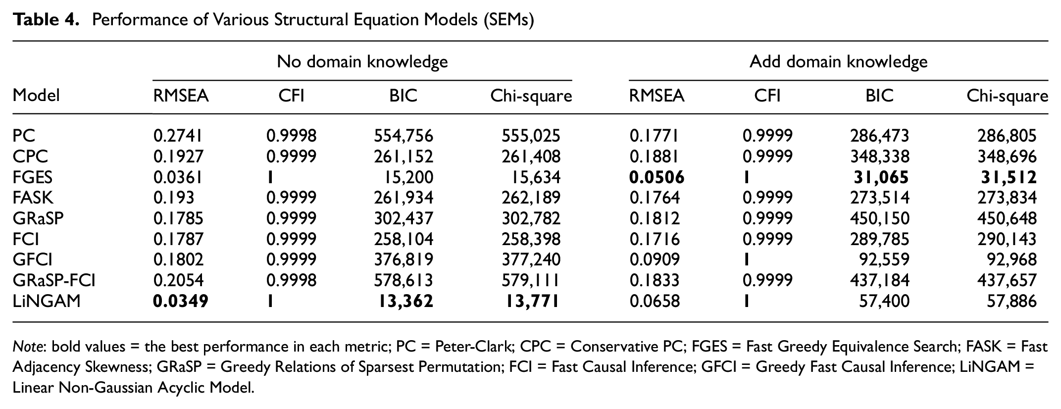
Tables 4 and 5 present the results of two types of evaluation metric. The bold values indicate the best performance in each metric. From Table 4, it is observed that both the FGES and LiNGAM models meet the acceptable criteria for RMSEA (< 0.06) and CFI (> 0.95), with LiNGAM performing slightly better than the FGES model. Similar results are reflected in the evaluation metrics presented in Table 5, where LiNGAM outperforms other models in the absence of domain knowledge. Therefore, when domain knowledge is not available, LiNGAM emerges as the superior model. This could be because LiNGAM emphasizes linear relationships, which can be more easily quantified and validated through GoF metrics. Additionally, LiNGAM is an FCM-based model, which infers causal relationships in a functional form, closely resembling the structure of SEM. As a result, it can better capture the causal structure.

Table 4.

Performance of Various Structural Equation Models (SEMs)

Model	No domain knowledge				Add domain knowledge
Model	RMSEA	CFI	BIC	Chi-square	RMSEA	CFI	BIC	Chi-square
PC	0.2741	0.9998	554,756	555,025	0.1771	0.9999	286,473	286,805
CPC	0.1927	0.9999	261,152	261,408	0.1881	0.9999	348,338	348,696
FGES	0.0361	1	15,200	15,634	0.0506	1	31,065	31,512
FASK	0.193	0.9999	261,934	262,189	0.1764	0.9999	273,514	273,834
GRaSP	0.1785	0.9999	302,437	302,782	0.1812	0.9999	450,150	450,648
FCI	0.1787	0.9999	258,104	258,398	0.1716	0.9999	289,785	290,143
GFCI	0.1802	0.9999	376,819	377,240	0.0909	1	92,559	92,968
GRaSP-FCI	0.2054	0.9998	578,613	579,111	0.1833	0.9999	437,184	437,657
LiNGAM	0.0349	1	13,362	13,771	0.0658	1	57,400	57,886

Note: bold values = the best performance in each metric; PC = Peter-Clark; CPC = Conservative PC; FGES = Fast Greedy Equivalence Search; FASK = Fast Adjacency Skewness; GRaSP = Greedy Relations of Sparsest Permutation; FCI = Fast Causal Inference; GFCI = Greedy Fast Causal Inference; LiNGAM = Linear Non-Gaussian Acyclic Model.

Table 5.

Performance of Various Causal Graph Models

Model	No domain knowledge					Add domain knowledge
Model	Error rate	Recall	Precision	Accuracy	F1	Error rate	Recall	Precision	Accuracy	F1
PC	47%	0.80	0.62	0.65	0.70	0.00	1.00	1.00	1.00	1.00
CPC	57%	0.70	0.54	0.55	0.61	0.00	1.00	1.00	1.00	1.00
FGES	52%	0.70	0.50	0.50	0.58	0.00	1.00	1.00	1.00	1.00
FASK	54.5%	0.80	0.62	0.65	0.70	0.00	1.00	1.00	1.00	1.00
GRaSP	46.4%	0.70	0.54	0.55	0.61	0.00	0.70	0.64	0.65	0.67
FCI	67.7%	0.40	0.31	0.25	0.35	0.00	1.00	1.00	1.00	1.00
GFCI	65.2%	0.40	0.44	0.45	0.42	0.00	0.80	1.00	0.90	0.89
GRaSP-FCI	55.6%	0.40	0.40	0.40	0.40	0.00	0.80	1.00	0.90	0.89
LiNGAM	43.5%	0.70	0.70	0.70	0.70	0.00	0.80	1.00	0.90	0.89

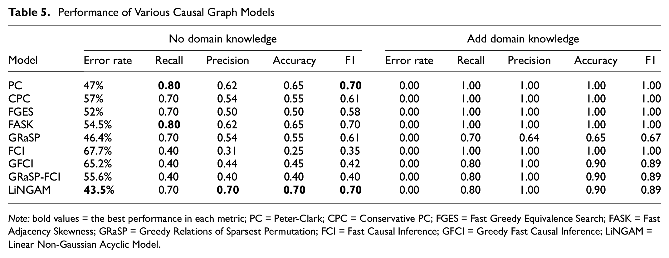
Note: bold values = the best performance in each metric; PC = Peter-Clark; CPC = Conservative PC; FGES = Fast Greedy Equivalence Search; FASK = Fast Adjacency Skewness; GRaSP = Greedy Relations of Sparsest Permutation; FCI = Fast Causal Inference; GFCI = Greedy Fast Causal Inference; LiNGAM = Linear Non-Gaussian Acyclic Model.

After incorporating domain knowledge, the evaluation results show a distinct pattern. When evaluating the model’s structure (see Table 4), it is observed that, while the performance of most models has significantly improved, FGES and LiNGAM show a relatively marginal decrease in performance. This can be attributed to the constraints (domain knowledge) applied to the model, which increases the number of parameters, making the FGES model more complex. The imposed hierarchical structure restricts the search space and prevents LiNGAM from finding the optimal structure. Despite this, these two models still outperform the others by a large margin, with FGES emerging as the superior model among them.

The performance of all models in Table 5 improves significantly after incorporating domain knowledge, showing almost perfect results. Notably, the error rate of all models drops to zero, which is attributed to domain knowledge correcting and eliminating many obvious false relationships. Moreover, except for GRaSP, all models achieved perfect precision (precision = 1), indicating that all false assertions were eliminated by the integration of domain knowledge. This improvement in model performance is also achieved by the incorporation of domain knowledge. The poor performance of GRaSP among these models is attributed to the current lack of implementation of forbidden edge knowledge (domain knowledge). In contrast, the higher recall indicates that most of the true assertion of causal relationships are accurately identified, which, to some extent, confirms the effectiveness of our assertions.

Causal Graph Visualization

This section visualizes the generated causal graphs and the inferred causal relationships based on the optimal causal discovery model evaluated in the previous section, and further explains the results. Concerning the choice of the optimal model, from Table 4, it is evident that, among the models evaluated, only FGES and LiNGAM satisfied the criteria for acceptability with RMSEA values < 0.06 and CFI values > 0.95. After integrating domain knowledge, FGES emerged as the superior model. Furthermore, as shown in Table 5, the performance of FGES consistently surpassed that of LiNGAM after the inclusion of domain knowledge. Based on these observations, we selected the FGES model to interpret the results.

Figures 4 and 5 visualize the causal graphs generated by the FGES model before and after the incorporation of domain knowledge, respectively. The edges within the graph represent causal relationships, where the direction of the arrow points to the effect, and the other side is the cause. The green numerals depicted in the figures correspond to the mean value of the respective variables. The numbers on the edges represent causal coefficients, illustrating the direct causal impact/strength between the two connected variables. 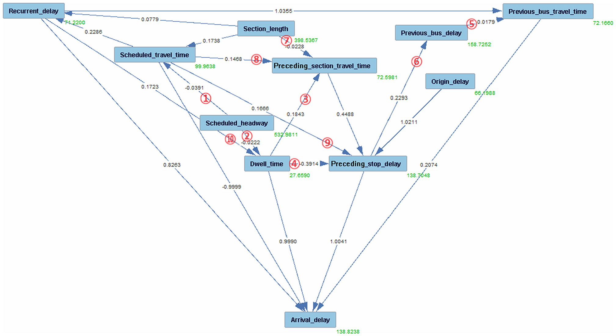More specifically, for a causal relationship $v_{i} \to v_{j}$ with a causal coefficient $α$ , a unit increment in $v_{i}$ will trigger an increase of $α$ units in $v_{j}$ regardless of the exogenous variables’ statistics, and regardless of whether the increment in $v_{i}$ is spurred by external manipulations or variations in exogenous variables.

Figure 4.

Graph generated from the fast greedy equivalence search model without domain knowledge.

Figure 5.

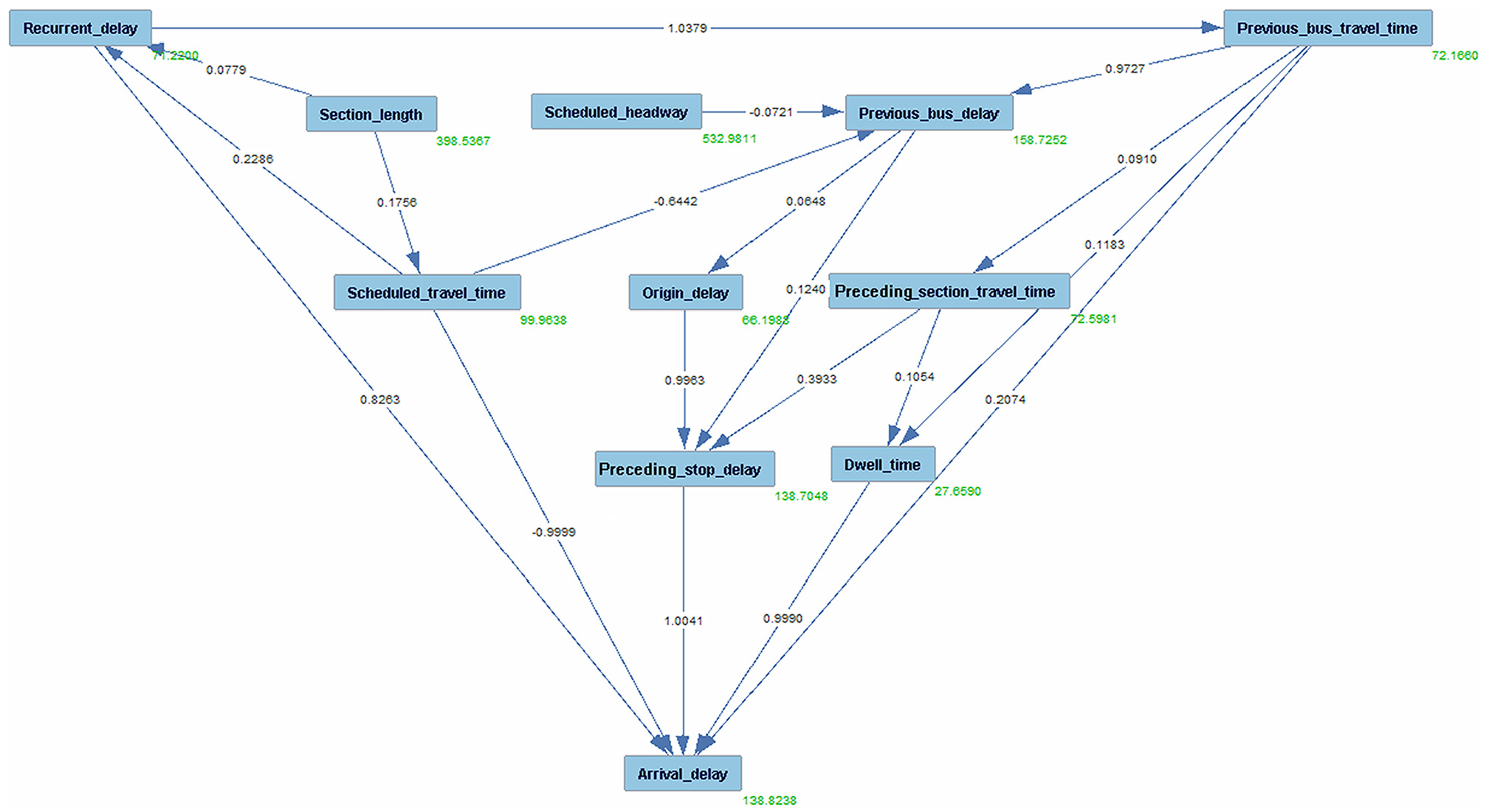
Graph generated from the fast greedy equivalence search model with domain knowledge.

The causal graph in Figure 4 shows many edges, including some obviously incorrect connections (labeled with red circle numbers) such as “dwell time → preceding stop delay and previous bus delay → previous bus travel time.”Figure 5 shows that the introduction of domain knowledge corrects the obvious incorrect connections in Figure 4 and introduces new and reasonable relationships, demonstrating an accurate understanding of the causal relationship between variables. To provide a clear comparison and to elucidate the enhancements brought by the incorporation of domain knowledge, Table 6 compares the relationships generated by the FGES model in the scenarios with and without domain knowledge. The comparison aims to highlight the differences in causal relationships, which are reflected in the correction of erroneous edges and the introduction of new, logically consistent edges, underlining the key role of domain knowledge in enhancing the accuracy and reliability of the inferred causal relationships.

Table 6.

Comparative Analysis of the Causal Graph (from the Fast Greedy Equivalence Search Model) with and without Domain Knowledge

Without domain knowledge		With domain knowledge
Relation	Coefficient	Relation	Coefficient
Same relations
Dwell time → arrival delay	0.999	Dwell time → arrival delay	0.999
Origin delay → preceding stop delay	1.0211	Origin delay → preceding stop delay	0.9963
Previous bus travel time → arrival delay	0.2074	Previous bus travel time → arrival delay	0.2074
Recurrent delay → arrival delay	0.8263	Recurrent delay → arrival delay	0.8263
Recurrent delay → previous bus travel time	1.0355	Recurrent delay → previous bus travel time	1.0379
Scheduled travel time → arrival delay	−0.9999	Scheduled travel time → arrival delay	−0.9999
Scheduled travel time → recurrent delay	0.2286	Scheduled travel time → recurrent delay	0.2286
Section length → recurrent delay	0.0779	Section length → recurrent delay	0.0779
Section length → scheduled travel time	0.1738	Section length → scheduled travel time	0.1756
Preceding stop delay → arrival delay	1.0041	Preceding stop delay → arrival delay	1.0041
Preceding section travel time → preceding stop delay	0.4488	Preceding section travel time → preceding stop delay	0.3933
Difference relations
Dwell time → preceding section travel time	0.1843	Previous bus delay → origin delay	0.0648
Dwell time → preceding stop delay	−0.3914	Previous bus delay → preceding stop delay	0.124
Previous bus delay → previous bus travel time	0.0179	Previous bus travel time → dwell time	0.1183
Recurrent delay → dwell time	0.1723	Previous bus travel time → previous bus delay	0.9727
Scheduled headway → dwell time	−0.0222	Preceding section travel time → dwell time	0.1054
Scheduled headway → scheduled travel time	−0.0391	Scheduled headway → previous bus delay	−0.0721
Scheduled travel time → preceding stop delay	0.1666	Scheduled travel time → previous bus delay	−0.6442
Scheduled travel time → preceding section travel time	0.1468	Previous bus travel time → preceding section travel time	0.091
Section length → preceding section travel time	−0.0228
Preceding stop delay → previous bus delay	0.2293

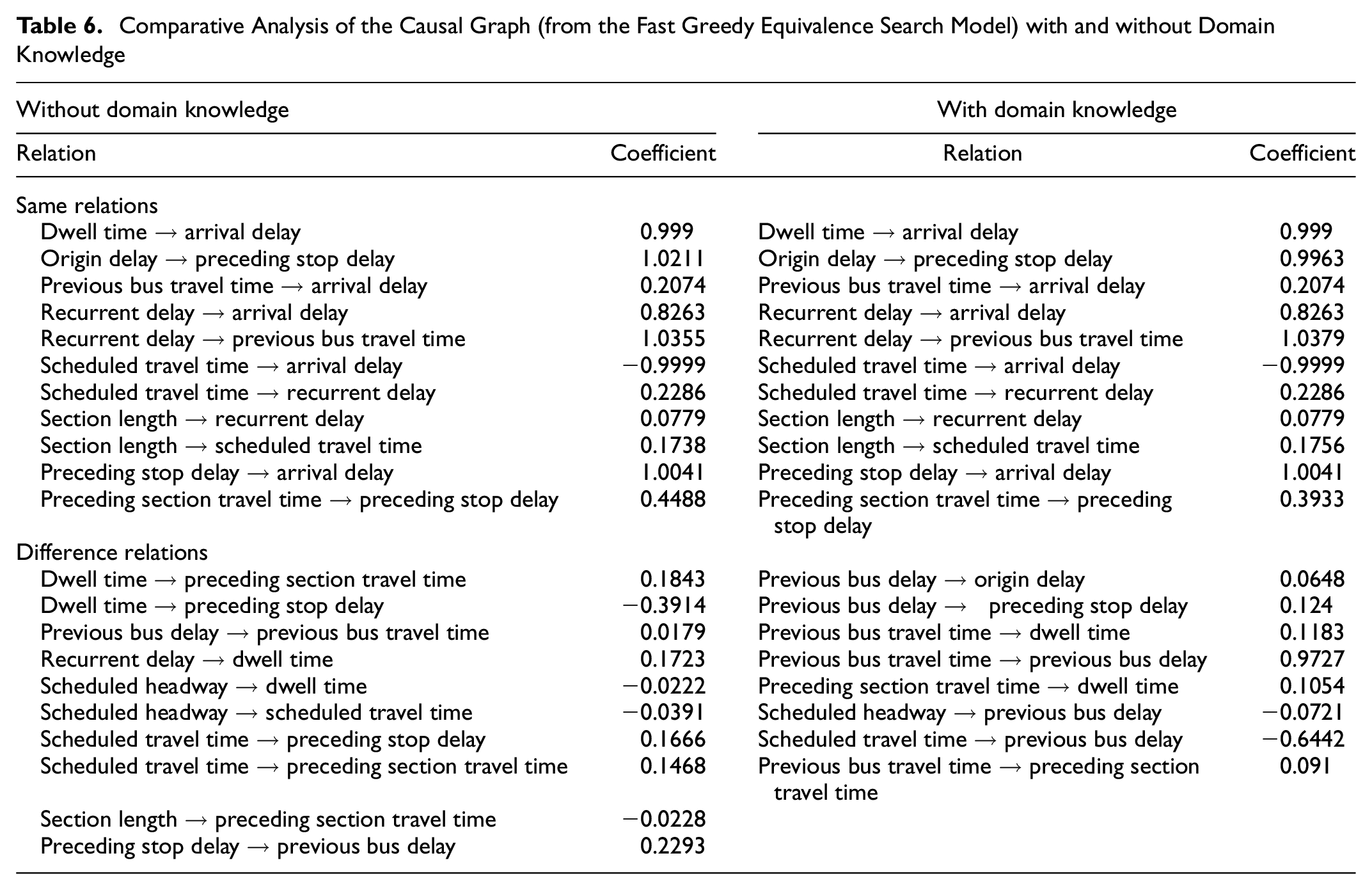
Table 5 lists the causal relationships shown in Figures 4 (right column) and 5 (left column). The “Same relations” refers to relations that appear in both figures, while the “Difference relations” indicate discrepancies between the relations in the two figures. The “Difference relations” are attributed to the incorporation of domain knowledge. All coefficients are statistically significant, with p-values < 0.05. The “Same relations” section of Table 6 highlights several causal relationships that remained consistent regardless of the incorporation of domain knowledge, underscoring the robustness of the FGES model in identifying these relationships. Furthermore, the inclusion of domain knowledge appears to have refined the coefficients of some relationships. For instance, the coefficient for the relationship “preceding section travel time → preceding stop delay” was adjusted from 0.4488 to 0.3933, indicating a more reasonable quantification of the causal effect. Incorporating domain knowledge makes the causal graph more reasonable; this, in turn, leads to more reasonable coefficient estimates in SEM. The “Difference relations” section unveils two aspects: firstly, the correction of causal directions (e.g., changing “previous bus delay → previous bus travel time” to “previous bus travel time → previous bus delay”), and, secondly, the identification of new causal relationships (e.g., “scheduled travel time → previous bus delay”).

In Figure 5, some findings can be observed. For example, preceding stop delay, dwell time, recurrent delay, and previous bus travel time exhibit strong positive direct causal effects on bus arrival delays (path coefficients of 1.004, 0.999, 0.826, and 0.207, respectively). Conversely, the scheduled travel time demonstrates a strong negative direct causal effect on bus arrival delays (−0.9999). These findings align with previous studies which identified significant correlations between these variables and bus arrival delays ( 17 , 18 ). Interestingly, the analysis reveals that origin delay, previous bus delay (knock-on delay), and preceding section travel time do not have a direct causal effect on bus arrival delays. Instead, they exert a direct causal influence on preceding stop delays, indirectly affecting bus arrival delays. Previous research supports the positive impact of origin delays and knock-on delays on arrival delays but does not provide insight into the specific pathways and causal relationships involved ( 16 ).

Moreover, the causal graph provides more profound insights into the interrelationships among variables, offering a more detailed and valuable perspective on the entire system. The causal graph in Figure 5 reveals that the previous bus travel time has a significant positive direct causal effect on the previous bus delay (with a path coefficient of 0.973), which suggests that longer travel times for the preceding bus can lead to increased delays in subsequent buses. Moreover, a strong positive causality coefficient (1.038) from recurrent delay to previous bus travel time suggests that recurrent delays (reflecting factors that frequently cause bus delays such as peak hours) have a significant effect on the previous bus travel time. This implies that, when recurrent delays occur, they are likely to contribute to an increase in the travel time of the previous bus. Furthermore, the scheduled travel time demonstrates a significant negative direct causal effect on the previous bus delay (with a path coefficient of −0.6442), which implies that longer scheduled travel times are associated with shorter delays in the previous bus.

Additionally, our analysis uncovers same slight direct causal effects, with path coefficients ranging between 0.1 and −0.1, among certain observed independent variables. For example, the scheduled headway exhibits a slight causal effect on the previous bus delay. This indicates that other unexplored factors (not considered in the current analysis) may have a more substantial impact on the variables under investigation. Therefore, further investigation and analysis are required to fully comprehend the nature and magnitude of these causal relationships.

Correlation Versus Causality

The purpose of this section is twofold. Firstly, it aims to demonstrate the important principle that “correlation does not imply causation.” More critically, we aim to explain the distinct differences and focuses between these two analytical approaches. This comparison is intended to serve as a reference for future researchers in choosing the most appropriate method for their studies.

Understanding the bus delay mechanism requires delving into the causal interactions among various factors, rather than just examining their correlations. Correlation analysis is a preliminary step in identifying potential associations between variables. Figure 6 shows the variables’ correlation matrix heatmap of the Pearson correlation coefficients, which shows the degree of linear relationship between two variables. Below is a comparison between causality and correlation.

Figure 6.

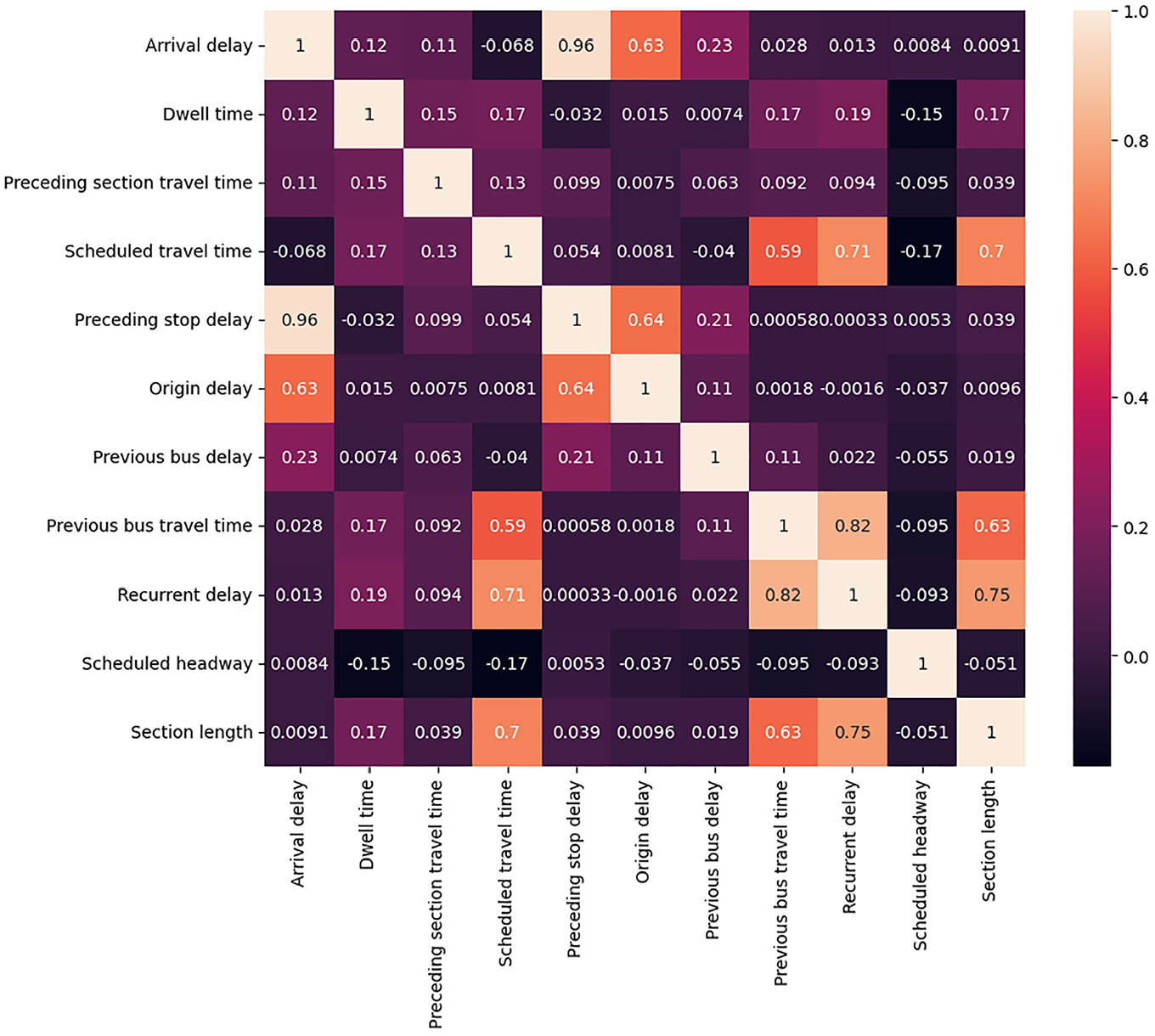
The heatmap of the correlation matrix.

Limited in Reflecting Interaction

Correlation, by its definition, is a statistical measure that describes the size and direction of a relationship between two or more variables ( 48 ). Correlation does not imply any causation. For instance, a notable high correlation of 0.63 is observed between “arrival delay” and “origin delay” (see Figure 6). Moreover, correlation analysis could be misleading in scenarios where a causal relationship does not manifest as a high correlation. For instance, the relationship between “arrival delay” and “scheduled travel time” shows a relatively low correlation of −0.068, yet, in the causal graph, a significant negative causal relationship is established with a path coefficient of −0.9999. This discrepancy underscores the limitation of correlation analysis in revealing the true nature of interactions among variables.

Lacks Directionality

Correlation measures the strength of the linear relationship between two quantitative variables, but it does not specify which variable is the cause and which is the effect; this relationship is symmetric. Causality establishes a directional and asymmetric relationship where one variable is deemed to directly influence the other. In causal relationships, there is an implied mechanism by which one variable (the cause) produces an effect on another variable (the effect), which can be demonstrated through interventions or experiments that manipulate the cause to observe changes in the effect. This distinction is crucial as correlation alone can be misleading, and the correlations may be spurious.

Unable to Reveal Influence Paths

Correlation does not reflect the influence path between variables; it merely indicates a linear relationship without implying direction, which is a crucial limitation in understanding the mechanism of bus delay propagation. Causality, identified through thorough analysis with causal discovery algorithms, provides deeper insights by establishing direct and indirect causal relationships that reflect the influence paths between variables. For example, the causal graph (see Figure 5) reveals an influence path: “origin delay → preceding stop delay → arrival delay,” which aids in understanding the mechanism of bus delay propagation.

Unable to Identify Confounders

Correlation falls short when it encounters confounding variables because it cannot reveal hidden relationships. Causality can handle confounding variables and provides a more reasonable representation of the true connection. FCI is adept at identifying hidden confounders among variables. For instance, in our study, we discern “previous bus delay ↔ preceding stop delay” using the FCI algorithm, where ↔ denotes the presence of an unmeasured confounder between the two variables. This observation aligns with reality, as traffic conditions or times of day (e.g., morning peak, afternoon peak) likely influence both “previous bus delay” and “preceding stop delay.”

In summary, while correlation analysis can provide a preliminary understanding of possible associations, it is the causal analysis that delves deeper into the underlying mechanics of bus delay propagation, offering a more reliable and insightful understanding. The comparison of coefficients from the correlation analysis and the path coefficients from the causal graph emphasizes the need to delve into causality in more detail, rather than just correlations, to fully understand bus delays.

Linear Regression (LR) versus Causality

In this section, we conduct cross-validation to compare LR (correlation-based) with causality-based analysis by examining the importance ranking of variables. The standardized coefficient is used to measure the relative importance and influence of independent variables (explanatory variables) on the outcome (i.e., bus arrival delays) ( 49 ).

We calculated the standardized coefficients for both LR and causal discovery model. Unlike LR, the causal effect includes both direct and indirect causal effects in causal analysis. For example, in the influence path “origin delay → preceding stop delay → arrival delay,” the variable “preceding stop delay” has a direct effect on arrival delays, while “origin delay” has an indirect effect. Moreover, some variables (e.g., “scheduled travel time”) have both direct and indirect effects. For example, “scheduled travel time” directly causes arrival delay and indirectly influences it through the path “scheduled travel time → recurrent delay → arrival delays.” In this case, the total effect of “scheduled travel time” is the sum of its direct and indirect effects. Figure 7 shows the variables’ importance ranking in LR and causality.

Figure 7.

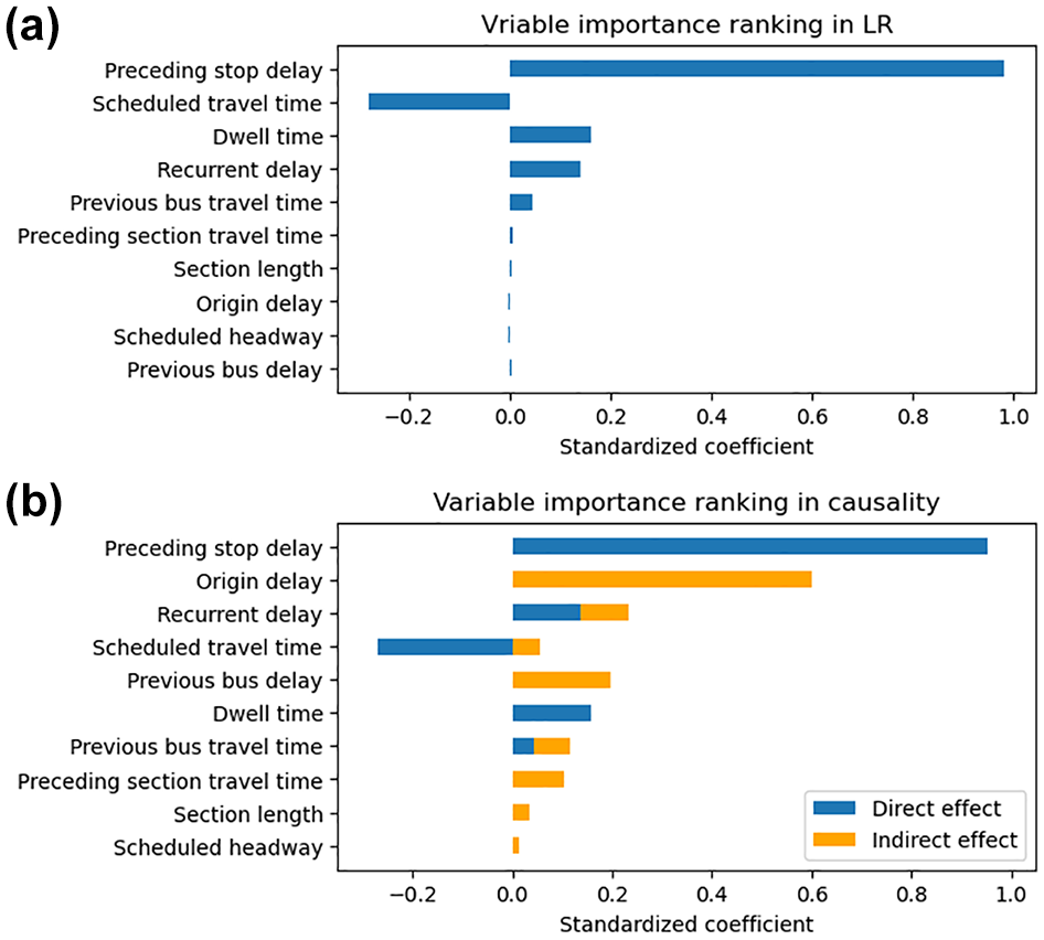
Linear regression (LR) versus causality—significance of variables: (a) LR model and (b) causal discovery model.

The comparison reveals notable differences in the importance rankings and influence magnitudes of the variables between the two models. Below, we provide a detailed comparison of these models.

Importance Ranking and Influence Magnitudes

A key distinction between the two models is the varied importance attributed to different factors. “Preceding stop delay” remains the most influential in both models (0.982 in LR, 0.954 in causality), but “origin delay” is markedly more significant in the causal graph (ranked 2nd at 0.601) compared with its lower rank (9th at 0.003) in LR. A limited number of studies have considered the initial stop’s delay across various contexts (e.g., bus bunching and travel time reliability) without directly studying their impact on bus delays. A related study indicates that a 1 min delay at the first stop typically results in a 0.633 min increase in travel time, which shows the importance of origin delays ( 50 ). Despite different rankings, “scheduled travel time” and “dwell time” show similar influence values, with −0.278 versus −0.215 (direct effect −0.269, indirect effect 0.054) and 0.161 versus 0.158 in LR and causality, respectively. Moreover, factors such as “previous bus delay,”“previous bus travel time,” and “preceding section travel time” receive more emphasis in the causality model. The primary distinction between the two models lies in the indirect effects captured by the causal models, while the direct effects are similar.

Influence Path

LR, a correlation-based model, primarily focuses on estimating the correlations between dependent and independent variables while controlling for other factors, essentially capturing the strength and direction of associations. In contrast, the causal analysis not only identifies direct effects but also unravels indirect relationships and influence path, offering a comprehensive understanding of how various factors interconnect and influence each other.

Robustness to Confounding

While LR can mitigate the effects of known confounders by incorporating them as covariates in the model, it lacks the intrinsic capability to detect or identify these confounding variables autonomously. This limitation requires prior knowledge of potential confounders in the data set, which makes it challenging in complex settings where unknown or unobserved confounders exist in reality. Therefore, the limitation can potentially lead to biased or misleading results.

Interventional Capability

LR is effective in analyzing and quantifying relationships within observational data but is limited in predicting the outcomes of interventions or changes, because of its reliance on existing data correlations. Causality, rooted in the principles of do-calculus, is pivotal for understanding how changes in one variable can actively influence outcomes ( 51 ). It is particularly useful for decision-making and policymaking, allowing researchers to simulate interventions and explore potential scenarios by asking “what if it was?” questions.

Predictive versus Interpretation

LR is often utilized for prediction, signifying how shifts in predictors are associated with changes in the outcome. Causality seeks to comprehend the actual causal mechanisms of the system, improving transparency and interpretability.

In summary, the LR model and the causal model are distinct analytical methods. LR excels at quantifying relationships between variables, focusing on observed correlations, and is primarily used for prediction. In contrast, the causal model delves into the underlying mechanisms, offering a deeper understanding of the direct and indirect effects between variables. It also has the ability to identify hidden confounding factors, enhancing interpretability. As Wasserman states, “Prediction is about passive observation, and causation is about active intervention” ( 52 ). This is the key distinction between the two models.

Discussion

This study highlights the significance of using causality to understand the factors contributing to bus delays. The increasing popularity of machine learning and deep learning techniques in the field has predominantly relied on correlation-based approaches, often overlooking the underlying causal relationships. By introducing a causality-based modeling approach, this study bridges this research gap and offers a novel perspective on analyzing bus arrival delays.

While automated causal graph discovery methods are widely utilized in mathematical and computer science domains, their application in constructing causal graphs for our specific research question has not been examined. To address this gap, we systematically evaluated the performance of typical causal discovery algorithms (e.g., PC, FGES, FCI) in the context of bus delays. Our results confirm that these algorithms can automatically generate causal graphs that reflect the underlying causal relationships among operational factors. However, the graphs generated by these methods sometimes contain erroneous directions and relationships. This suggests that they do not always fully capture the complex causal dynamics inherent in bus delay systems.

To enhance the accuracy and effectiveness of these automated methods, we advocate for incorporating domain expertise to refine and correct the relations generated in the causal graph. This process empowers the learning process, facilitating the construction of causal graphs. It addresses the limitations observed in purely automated approaches, generating more accurate and insightful causal graphs that capture the interrelationships of variables as well as the relationships between operational variables and bus delays. Empirically, we validated the generated causal graphs by comparing them against our domain knowledge and intuition about real-world relationships. This demonstrates that the generated graphs effectively capture both expected and unexpected relationships, aligning with reality. It underscores the robustness of causal approach in identifying and representing causal relationships that significantly affect bus delays.

The causal graph provides a visual representation of the complexity inherent in bus arrival delays, enhancing the explainability of the modeling results. The direct causal links between operational factors and bus delays provide empirical evidence for making prioritized and targeted interventions. For example, we found that preceding stop delay, dwell time, recurrent delay, and previous bus travel time have a strong positive direct causal effect on bus arrival delays, while scheduled travel time exhibits a strong negative direct causal effect. This suggests it is important to focus on these variables to develop target strategies to mitigate delays directly. Moreover, causal graphs offer a more comprehensive view that goes beyond traditional correlation-based methods. They not only detail the relationships between variables but also unveil the influence path, revealing how various intricately contribute to bus delays. For example, origin and previous bus delays significantly influence preceding stop delays, indirectly affecting bus arrival times. This insight helps identify primary delay causes and strategies to reduce delay spread across the network. More importantly, the interventionable capability enables causal models to simulate interventions on the causes to observe changes in the outcomes, which is particularly useful to answer “what if it was?” questions.

Conclusion

This study introduces causal graph discovery algorithms to comprehensively investigate the causal factors influencing bus delays using GTFS data. We explore nine causal discovery algorithms to generate causal graphs of bus arrival delays and assess their performance in both statistical data fitting (metrics including RMSE, CFI, BIC, TEC) and causality interpretation (metrics including accuracy rate, recall, precision, etc.). The empirical analysis is conducted using GTFS data collected from high-frequency bus routes in Stockholm, Sweden. The comparison analysis shows that the FGES model performs the best in data fitting and discovering correct causal relationships. SEM is used to quantify the causal strength of the causal links, making it possible to identify and explore significant causal links and their practical implications. The findings highlight the complexity of factors contributing to bus delays and emphasize the importance of introducing causality into bus delay factor analysis.

Comparing with traditional correlation-based methods (e.g., Pearson correlation and LR) shows that a high correlation does not imply a strong causation, and, conversely, weak correlations do not imply a lack of causation. Moreover, the indirect effects are an undeniable influence that plays a vital role in illuminating the interconnected nature of variables and their cumulative impact on outcomes. These insights are crucial for decision-making and policy formulation in bus operations. It suggests that reliance solely on correlation, statistical analysis, and machine-learning-based models may not lead to optimal decisions. More significantly, causal models can identify hidden or unmeasured confounders, a capability absent in other methodologies. Confounders are the main source of spurious correlations. This attribute is pivotal in enhancing the accuracy of causal inference, thereby playing a critical role in a fundamental understanding of the system’s mechanisms.

Additionally, this study utilizes open-source Python packages to implement the framework in practice (a detailed description can be found in the Results subsection), similar to other regression analysis models. This accessibility enables researchers and practitioners to apply the framework to infer causal relationships, visualize causal graphs, and quantify causal effects, providing a powerful tool for analyzing specific problems in their field.

While this study provides valuable insights, it has limitations. We are attempting to introduce causal graphs to address our research problem. This study is the first step in this direction, but the final causal graph proposed may not be the optimal one. Alternative causal discovery models might provide a more precise representation of the causality. Furthermore, this study concentrates on specific variables, while acknowledging that other influential factors not included in our analysis should be taken into consideration, as they may also affect bus delays. Subsequent research should endeavor to validate the identified causal relationships across diverse contexts and consider incorporating supplementary factors to deepen the comprehension of bus delays.

Supplemental Material

sj-pdf-1-trr-10.1177_03611981241306754 – Supplemental material for Causal Graph Discovery for Urban Bus Operation Delays: A Case Study in Stockholm

Supplemental material, sj-pdf-1-trr-10.1177_03611981241306754 for Causal Graph Discovery for Urban Bus Operation Delays: A Case Study in Stockholm by Qi Zhang, Zhenliang Ma, Yancheng Ling, Zhenlin Qin, Pengfei Zhang and Zhan Zhao in Transportation Research Record

Footnotes

Author Contributions

The authors confirm contribution to the paper as follows: study conception and design: Qi Zhang, Zhenliang Ma; data collection: Yancheng Ling, Zhenlin Qin; analysis and interpretation of results: Qi Zhang, Zhenliang Ma, Pengfei Zhang, Zhan Zhao; draft manuscript preparation: Qi Zhang. All authors reviewed the results and approved the final version of the manuscript.

Declaration of Conflicting Interests

The author(s) declared no potential conflicts of interest with respect to the research, authorship, and/or publication of this article.

Funding

The author(s) disclosed receipt of the following financial support for the research, authorship, and/or publication of this article: This work was supported by the China Scholarship Council under Grant No. 202006950007 and KTH Digital Futures (cAIMBER).

ORCID iDs

Zhenliang Ma

Yancheng Ling

Zhenlin Qin

Zhan Zhao

References

Amberg

Kliewer

Robust Efficiency in Urban Public Transportation: Minimizing Delay Propagation in Cost-Efficient Bus and Driver Schedules. Transportation Science, Vol. 53, No. 1, 2019, pp. 89–112.

Barabino

Di Francesco

Mozzoni

Rethinking Bus Punctuality by Integrating Automatic Vehicle Location Data and Passenger Patterns. Transportation Research Part A: Policy and Practice, Vol. 75, 2015, pp. 84–95.

Z.-L.

Ferreira

Mesbah

Hojati

A. T.

Modeling Bus Travel Time Reliability with Supply and Demand Data from Automatic Vehicle Location and Smart Card Systems. Transportation Research Record: Journal of the Transportation Research Board, 2015. 2533: 17–27.

Zhu

Koutsopoulos

H. N.

Ferreira

Quantile Regression Analysis of Transit Travel Time Reliability with Automatic Vehicle Location and Farecard Data. Transportation Research Record: Journal of the Transportation Research Board, 2017. 2652: 19–29.

Kathuria

Parida

Chalumuri

R. S.

Travel-Time Variability Analysis of Bus Rapid Transit System Using GPS Data. Journal of Transportation Engineering, Part A: Systems, Vol. 146, No. 6, 2020, p. 05020003.

Chen

Zhang

Guo

Analyzing Urban Bus Service Reliability at the Stop, Route, and Network Levels. Transportation Research Part A: Policy and Practice, Vol. 43, No. 8, 2009, pp. 722–734.

Holland

P. W.

Statistics and Causal Inference. Journal of the American Statistical Association, Vol. 81, No. 396, 1986, pp. 945–960.

Huang

Chen

Sumalee

Pan

Zhong

Bus Arrival Time Prediction and Reliability Analysis: An Experimental Comparison of Functional Data Analysis and Bayesian Support Vector Regression. Applied Soft Computing, Vol. 111, 2021, p. 107663.

Rodriguez-Deniz

Villani

Robust Real-Time Delay Predictions in a Network of High-Frequency Urban Buses. IEEE Transactions on Intelligent Transportation Systems, Vol. 23, No. 9, 2022, pp. 16304–16317.

10.

Singh

Kumar

A Review of Bus Arrival Time Prediction Using Artificial Intelligence. Wiley Interdisciplinary Reviews: Data Mining and Knowledge Discovery, Vol. 12, No. 4, 2022, p. e1457.

11.

Wood

J. S.

Gayah

V. V.

Using Survival Models to Estimate Bus Travel Times and Associated Uncertainties. Transportation Research Part C: Emerging Technologies, Vol. 74, 2017, pp. 366–382.

12.

Jiang

Lam

S.-K.

Sun

Learning Heterogeneous Traffic Patterns for Travel Time Prediction of Bus Journeys. Information Sciences, Vol. 512, 2020, pp. 1394–1406.

13.

Soza-Parra

Muñoz

J. C.

Raveau

Factors that Affect the Evolution of Headway Variability Along an Urban Bus Service. Transportmetrica B: Transport Dynamics, Vol. 9, No. 1, 2021, pp. 479–490.

14.

Park

Mount

Liu

Xiao

Miller

H. J.

Assessing Public Transit Performance Using Real-Time Data: Spatiotemporal Patterns of Bus Operation Delays in Columbus, Ohio, USA. International Journal of Geographical Information Science, Vol. 34, No. 2, 2020, pp. 367–392.

15.

Yang

Qian

Understanding and Predicting Travel Time with Spatio-Temporal Features of Network Traffic Flow, Weather and Incidents. IEEE Intelligent Transportation Systems Magazine, Vol. 11, No. 3, 2019, pp. 12–28.

16.

Schmöcker

J.-D.

Sun

Fonzone

Liu

Bus Bunching Along a Corridor Served by Two Lines. Transportation Research Part B: Methodological, Vol. 93, 2016, pp. 300–317.

17.

Strathman

J. G.

Kimpel

T. J.

Dueker

K. J.

Gerhart

R. L.

Callas

Evaluation of Transit Operations: Data Applications of Tri-Met’s Automated Bus Dispatching System. Transportation, Vol. 29, 2002, pp. 321–345.

18.

Luo

Liu

Jin

Bus Queue Time Estimation Model for a Curbside Bus Stop Considering the Blocking Effect. Scientific Reports, Vol. 12, No. 1, 2022, p. 11576.

19.

Haig

B. D.

What is a Spurious Correlation?

Understanding Statistics: Statistical Issues in Psychology, Education, and the Social Sciences, Vol. 2, No. 2, 2003, pp. 125–132.

20.

Bareinboim

Pearl

Controlling Selection Bias in Causal Inference. Proc., Fifteenth International Conference on Artificial Intelligence and Statistics, PMLR, Canary Islands, Spain, 2012, pp. 100–108.

21.

Ullman

J. B.

Bentler

P. M.

Structural Equation Modeling. In Handbook of Psychology ( J. A.

Schinka

Velicer

W. F.

Weiner

I. B.

, eds.), 2nd ed., Vol. 2, John Wiley & Sons, Inc., New Jersey, 2012, pp. 661–690.

22.

Wang

Yan

Zhou

Xue

Influencing Mechanism of Potential Factors on Passengers’ Long-Distance Travel Mode Choices Based on Structural Equation Modeling. Sustainability, Vol. 9, No. 11, 2017, p. 1943.

23.

Golob

T. F.

Structural Equation Modeling for Travel Behavior Research. Transportation Research Part B: Methodological, Vol. 37, No. 1, 2003, pp. 1–25.

24.

Guo

Cheng

Hahn

P. R.

Liu

A Survey of Learning Causality with Data: Problems and Methods. ACM Computing Surveys (CSUR), Vol. 53, No. 4, 2020, pp. 1–37.

25.

Triantafillou

Tsamardinos

Score-Based vs Constraint-Based Causal Learning in the Presence of Confounders. In Cfa@uai, Proc., 32 Conference on Uncertainty in Artificial Intelligence (UAI 2016), New York City, NY, 2016, pp. 59–67.

26.

Wang

Pan

Tian

Zhang

Conditional Distance Correlation. Journal of the American Statistical Association, Vol. 110, No. 512, 2015, pp. 1726–1734.

27.

Runge

Nowack

Kretschmer

Flaxman

Sejdinovic

Detecting and Quantifying Causal Associations in Large Nonlinear Time Series Datasets. Science advances, Vol. 5, No. 11, 2019, p. eaau4996.

28.

Strobl

E. V.

Zhang

Visweswaran

Approximate Kernel-Based Conditional Independence Tests for Fast Non-Parametric Causal Discovery. Journal of Causal Inference, Vol. 7, No. 1, 2019, p. 20180017.

29.

Spirtes

Glymour

C. N.

Scheines

Causation, Prediction, and Search. MIT Press, Cambridge, MA, 2000.

30.

Ramsey

Zhang

Spirtes

P. L.

Adjacency-Faithfulness and Conservative Causal Inference. arXiv preprint arXiv:1206.6843, 2012.

31.

Neath

A. A.

Cavanaugh

J. E.

The Bayesian Information Criterion: Background, Derivation, and Applications. Wiley Interdisciplinary Reviews: Computational Statistics, Vol. 4, No. 2, 2012, pp. 199–203.

32.

Akaike

Information Theory and an Extension of the Maximum Likelihood Principle. In Selected Papers of Hirotugu Akaike ( E.

Parzen

Tanabe

Kitagawa

, eds.), Springer, New York, NY, 1998, pp. 199–213.

33.

Buntine

Theory Refinement on Bayesian Networks. Uncertainty Proceedings 1991, Morgan Kaufmann, MA 1991, pp. 52–60.

34.

Ramsey

Glymour

Sanchez-Romero

Glymour

A Million Variables and More: the Fast Greedy Equivalence Search Algorithm for Learning High-Dimensional Graphical Causal Models, With an Application to Functional Magnetic Resonance Images. International Journal of Data Science and Analytics, Vol. 3, 2017, pp. 121–129.

35.

Zhang

Wang

Zhang

Schölkopf

On Estimation of Functional Causal Models: General Results and Application to the Post-Nonlinear Causal Model. ACM Transactions on Intelligent Systems and Technology (TIST), Vol. 7, No. 2, 2015, pp. 1–22.

36.

Shimizu

Hoyer

P. O.

Hyvärinen

Kerminen

Jordan

A Linear Non-Gaussian Acyclic Model for Causal Discovery. Journal of Machine Learning Research, Vol. 7, No. 10, 2006, pp. 2003–2030.

37.

Ogarrio

J. M.

Spirtes

Ramsey

A Hybrid Causal Search Algorithm for Latent Variable Models. Proc., Conference on Probabilistic Graphical Models, PMLR, Lugano, Switzerland, 2016, pp. 368–379.

38.

Lam

W.-Y.

Andrews

Ramsey

Greedy Relaxations of the Sparsest Permutation Algorithm. Proc., Uncertainty in Artificial Intelligence, PMLR, Eindhoven, The Netherlands, 2022, pp. 1052–1062.

39.

Sanchez-Romero

Ramsey

J. D.

Zhang

Glymour

M. K.

Huang

Glymour

Causal Discovery of Feedback Networks with Functional Magnetic Resonance Imaging. bioRxiv, 2018, p. 245936.

40.

Kline

R. B.

Principles and Practice of Structural Equation Modeling. Guilford Publications, New York, 2023.

41.

Chauhan

R. S.

Riis

Adhikari

Derrible

Zheleva

Choudhury

C. F.

Pereira

F. C.

Causality in Travel Mode Choice Modeling: A Novel Methodology that Combines Causal Discovery and Structural Equation Modeling. arXiv preprint arXiv:2208.05624, 2022.

42.

Cats

Loutos

Real-Time Bus Arrival Information System: An Empirical Evaluation. Journal of Intelligent Transportation Systems, Vol. 20, No. 2, 2016, pp. 138–151.

43.

Rigdon

E. E.

CFI Versus RMSEA: A Comparison of Two Fit Indexes for Structural Equation Modeling. Structural Equation Modeling: A Multidisciplinary Journal, Vol. 3, No. 4, 1996, pp. 369–379.

44.

Powers

D. M. W.

Evaluation: From Precision, Recall and F-Measure to ROC, Informedness, Markedness and Correlation. arXiv Preprint arXiv:2010.16061, 2011.

45.

Glick

T. B.

Figliozzi

M. A.

Measuring the Determinants of Bus Dwell Time: New Insights and Potential Biases. Transportation Research Record: Journal of the Transportation Research Board, 2017. 2647: 109–117.

46.

Ramsey

Andrews

Py-Tetrad and RPy-Tetrad: A New Python Interface with R Support for Tetrad Causal Search. In Causal Analysis Workshop Series, PMLR, Vol. 223, 2023, pp. 40–51.

47.

Igolkina

A. A.

Meshcheryakov

semopy: A Python Package for Structural Equation Modeling. Structural Equation Modeling: A Multidisciplinary Journal, Vol. 27, No. 6, 2020, pp. 952–963.

48.

Goodwin

L. D.

Leech

N. L.

Understanding Correlation: Factors that Affect the Size of r. The Journal of Experimental Education, Vol. 74, No. 3, 2006, pp. 249–266.

49.

Lleras

Path Analysis. Encyclopedia of Social Measurement, Vol. 3, No. 1, 2005, pp. 25–30.

50.

Kutlimuratov

Mukhitdinov

Impact of Stops for Bus Delays on Routes. IOP Conference Series: Earth and Environmental Science, Vol. 614, 2020, p. 012084.

51.

Pearl

Bareinboim

External Validity: from do-Calculus to Transportability Across Populations. Statistical Science, Vol. 29, No. 4, 2014, pp. 579–595.

52.

Naser

Causality and Causal Inference for Engineers: Beyond Correlation, Regression, Prediction and Artificial Intelligence. Wiley Interdisciplinary Reviews: Data Mining and Knowledge Discovery, Vol. 14, No. 4, 2024, p. e1533.

Supplementary Material

Please find the following supplemental material available below.

For Open Access articles published under a Creative Commons License, all supplemental material carries the same license as the article it is associated with.

For non-Open Access articles published, all supplemental material carries a non-exclusive license, and permission requests for re-use of supplemental material or any part of supplemental material shall be sent directly to the copyright owner as specified in the copyright notice associated with the article.

0.00 MB

0.68 MB