
Abstract
The transportation sector in the United States has faced funding challenges owing to a stagnant federal fuel tax rate and rising vehicle fuel economy. To address this issue, policy makers have explored the potential of a vehicle miles traveled (VMT) fee as an alternative funding method. However, equity concerns remain across income and geographic groups. This study explored equity issues with a VMT fee for different income levels and two geographic groups (urban and rural), in four states (California [CA], Iowa [IA], New York [NY], and Texas [TX]). Using 2009 and 2017 National Household Travel Survey data, the study analyzed VMT demand elasticity using structural equation modeling and applied it to VMT fee scenarios. The results showed that the current fuel tax system charges higher-income and urban households more than lower-income and rural households, whereas the VMT fee system reduced these differences a small amount. Households in CA, IA, NY, and TX paid, on average, $10, $5, $2, and $2 less per year with the VMT fee, respectively, compared with the current fuel tax system. This is primarily since electric vehicles will also pay the VMT fee. Most importantly, the difference in the amount paid changed very little under a VMT fee for the different income and geographic traveler segments, potentially alleviating some equity concerns.
Keywords
In the United States, gasoline and diesel taxes have been depreciating in real value for decades as the federal fuel tax has been 18.4 cents/gal (for gasoline) and 24.3 cents/gal (for diesel) since 1993 ( 1 ). Since 2001, the federal government’s primary funding source for transportation infrastructure, the Highway Trust Fund, has been decreasing with insufficient fuel tax revenue playing a major role ( 2 ). Moreover, owing to the rising fuel economy of vehicles and the increased numbers of electric and hybrid vehicles, the link between the gas tax and infrastructure use is weakening, rendering drivers less accountable for damage to roadway ( 3 ). Thus, the combination of stagnant tax rates, rising fuel efficiency, and inflation has degraded the purchasing power of the tax rates by over 30% ( 4 ).
Compounding these financial challenges, the transportation sector is a significant producer of greenhouse gas emissions, accounting for approximately 29% of total emissions ( 5 ). Driving also significantly contributes to externalities such as congestion, pollution, and traffic accidents, which cost American society hundreds of billions of dollars annually ( 6 ). Based on these issues, economists have focused on analyzing policies to reduce pollution and have long argued that gasoline taxes are more effective than corporate average fuel economy standards because they encourage drivers to reduce their vehicle miles traveled (VMT), as well as to increase the fuel efficiency of their vehicles ( 1 ). However, despite its effectiveness, increasing the gas tax, especially at the federal level, has proven to be politically challenging.
Given the challenges of declining transportation revenue, environmental concerns, and the need for effective policy tools, many policy makers and researchers have focused on a per-mile fee, or mileage-based user fee (MBUF), as a potential solution. Oregon ( 7 ), Utah ( 8 ), and Virginia ( 9 ) have already introduced an MBUF program on a small scale but permanent basis. Hawaii and Vermont have passed laws to impose MBUF on electric vehicles (EVs) starting from July 2025 (U.S. Department of Energy, 2023) ( 10 , 11 ). Pilot projects to demonstrate VMT-based fees have also been conducted in several states in the United States including Oregon, Minnesota, Colorado, Washington, California, and Hawaii ( 12 ), whereas Kansas ( 13 ), Connecticut ( 14 ), and Georgia ( 15 ) are operating ongoing pilot projects as of November 2023. For heavy vehicles and commercial trucks, the VMT-based fee is charged according to the weight of vehicles in four states: Oregon, New Mexico, Kentucky, and New York ( 2 , 16 , 17 ).
However, the distributional implications of this tax policy change are uncertain and raise equity concerns across different income levels and regional groups ( 18 ). Researchers investigated the distributional impact of VMT fees replacing the gas tax and found conflicting findings. One study found that the VMT tax is less regressive than an emissions tax (which is similar to but not the same as a gas tax) ( 19 ). Similarly, studies have also found that the VMT tax shifts the tax burden from low- to high-income households ( 18 , 20 ). In contrast, several studies have shown that the VMT tax is more regressive than the fuel tax ( 21 ), disproportionately burdening the lower-income groups. It is therefore crucial to investigate who will pay more and who will pay less in the new tax policy. To further investigate this ambiguity, this study explored the equity perspective of the VMT-based fee for different income and regional groups (urban and rural) using two waves of the National Household Travel Survey (NHTS) data from 2009 and 2017 for four states: California (CA), Iowa (IA), New York (NY), and Texas (TX). These states were selected (1) for geographic representation from around the United States, (2) because each has many responses in the NHTS dataset, and (3) because they have variation in their fuel tax levels, average VMT, and average fuel efficiency. However, this study investigated two dimensions of equity in the context of VMT fees: vertical equity, which addresses the fairness of tax burden across different income levels ( 22 ), and geographic equity, which assesses the regional disparities in tax policy impacts ( 23 ).
This study included two scenarios for analysis: static and dynamic. For the static scenario, people were assumed not to change their VMT in the new tax system, whereas in the dynamic scenario they were anticipated to change their VMT in response to the price change. The change in VMT resulting from the price change was determined from the elasticities of a structural equation model for VMT demand for different income classes of people living in both urban and rural areas. In general, as the price of fuel increases the amount of fuel purchased should decrease along with the amount of vehicle travel. However, the elasticity of demand is likely to vary by income group and geographic location. For example, higher-income groups may be less elastic, since they can more readily afford this change in cost. Conversely, urban travelers may have higher elasticities since they may have more travel options available, such as transit. Therefore, for the dynamic scenario, the elasticity of demand was calculated for each income and geographic group.
There are several studies that have investigated the elasticity of VMT demand from price change. Most of these studies used cross sectional data ( 24 ), time-series data ( 25 ), or panel data ( 26 ). Wang and Chen developed a structural equation model to calculate the elasticities for different income groups in which the potential endogeneity of fuel efficiency and VMT was also considered using the 2009 NHTS ( 24 ). The elasticity values ranged from −0.011 to −0.700 depending on the income levels. Although most of the research in this field found elasticity to be in the range of −0.2 to −0.5 ( 6 ), Weatherford found that the mean price elasticity of −1.48 was overestimated using 2009 NHTS data ( 18 ). Langer et al. conducted a disaggregate analysis and developed a VMT demand model using individual driver’s VMT using monthly panel data and found the elasticity value of −0.117 ( 1 ). Another study by Ju et al. estimated elasticities using 2017 NHTS data and found elasticities to be in the range of −0.28 to 0.22 across different income groups and two regional groups: urban and rural ( 27 ) . The problem with 1-year cross sectional data is that it cannot capture large price variations among households, potentially leading to poor estimates of elasticity. There were limited studies that explored elasticity using multiple years of data from the NHTS. One recent study by Goetzke and Vance used 2009 and 2017 NHTS data and developed three estimators—ordinary least squares (OLS), quantile regression, and instrumenting gas price with internationally traded oil—and found elasticity values of −0.050 to −0.291 ( 28 ). Our research used similar techniques but focused on four different regions (states) in the United States.
Our current study examined the elasticity using NHTS data from 2 years (2009 and 2017) and calculated the tax burden for residents in urban and rural regions for four different states with distinct geographic settings. These four states collected additional data as part of the NHTS, providing a large enough sample size for each state.
Data
National Household Travel Survey
The 2009 and 2017 NHTSs were used for modeling the VMT function, and the 2017 dataset was used for the analysis of the VMT fee. At the time of writing, the 2017 NHTS data is the latest version of the survey, however, the most recent two datasets were used in this study to capture people’s reaction to the fuel price change. Both datasets include several common data elements such as the annual VMT, the fuel economy of each vehicle, household income level, household location (i.e., urban or rural), the number of household members, the number of vehicles, the number of adults, and the number of drivers in each household. In the 2017 NHTS data, the fuel type information includes one category that combined EVs with hybrid vehicles. Since the data were combined, this research made the assumption that all vehicles in that category were electric. Because the fuel consumption of hybrid vehicles was not considered in the current fuel tax scenario, the current tax burden by household might be estimated at a slightly lower level than the actual tax burden in the real world.
The NHTS’s technical note ( 29 ) recommends increasing the 2017 annual mileage data by 10% when comparing it with mileage data from previous years, because of a difference in data collection techniques. Therefore, we applied this 10% increase to the 2017 annual mileage data when estimating fuel price elasticity using both the 2009 and 2017 NHTS data. In addition, the impact of inflation was mitigated by adjusting the income and gas price values in the 2009 dataset with the consumer price index (CPI). The source of the CPI is the Bureau of Labor Statistics ( 30 ). As specified, this study selected four states: CA, IA, NY, and TX. Across these states, 59,918 households with 127,843 vehicles in the 2009 dataset, and 53,685 households with 111,564 vehicles in the 2017 dataset were analyzed.
Fuel Tax
This study assumed that the VMT fee would replace the current state fuel tax and generate the same gross revenues. The state fuel tax levels by fuel type and year for each state were available from the Federal Highway Administration’s website ( 31 ). These were used to calculate the current state fuel tax revenue from the sample of NHTS vehicles. The VMT fee was then set in each state such that the NHTS vehicles from that state would generate the same revenue as they did under the current state gas tax. In 2017, state fuel tax for gasoline (diesel) was $ 0.42/gal ($ 0.36/gal) in CA, $ 0.315/gal ($ 0.335/gal) in IA, $ 0.24/gal ($ 0.22/gal) in NY, and $ 0.2/gal ($ 0.2/gal) in TX. CA’s fuel tax was the highest whereas TX showed the lowest level of state fuel tax for both gasoline and diesel.
Methodology
To begin, households were classified into five income groups and two regional groups (rural and urban) since fuel price elasticities, VMTs, and fuel economies were expected to differ by income and regional group. Five income groups were defined so that approximately 20% of households were in each income group in each state. Therefore, the income group range differed by state and analysis as shown in Table 1. For the VMT fee analysis, households were classified into five income groups using only the 2017 NHTS data, whereas the combined dataset was used in the income group classification for the elasticity calculation. For income group classification of the combined dataset, the 2009 income data were adjusted using the CPI as discussed below. Classifying each household as rural or urban was based on the data provided in the NHTS. The regional classification of urban and rural areas for 2009 NHTS data followed the 2000 U.S. census, whereas the 2017 NHTS data followed the 2014 TIGER/Line shapefiles that were also provided by via U.S. census data (NHTS). There were 40,865 urban households and 9,475 rural households in our final set of data.
Annual Household Income Ranges by Analysis and State (US$)
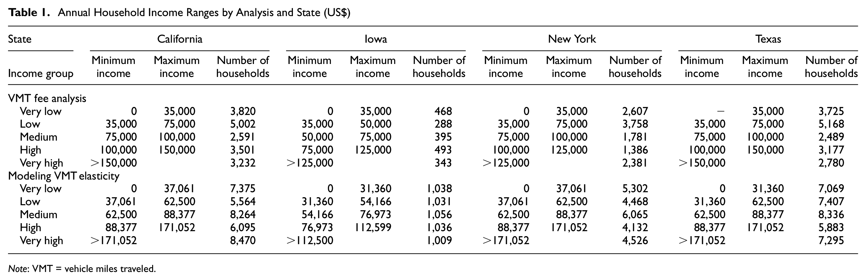
Note: VMT = vehicle miles traveled.
Data Preprocessing
Missing Values and Outliers
In this study, VMT, income class, the location of the household (rural/urban), fuel economy, and cost per mile were necessary for both elasticity calculations and the analysis of the VMT fee. Therefore, households missing any of those values were removed. In elasticity modeling, additional variables related to each household were included, such as household size, number of vehicles, -drivers, -workers, -adults, the population density of the region in which the household is situtated, and vehicle age. Households with missing values for these additional variables were excluded from the elasticity estimation process.
Outliers were also removed based on three criteria. First, households with an annual VMT of less than 100 mi were removed. Second, all households with an annual VMT per driver of more than 67,500 mi were removed. Third, households whose number of vehicles was greater than 2.5 times the number of household members or three times the number of adults were removed. Using these criteria, 287 vehicles were removed from a total sample of 91,942 vehicles (0.3%).
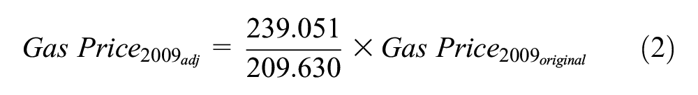
Inflation Adjustment
To account for inflation, the income level and gas price information in the 2009 dataset were adjusted into the 2017 level using Equations 1 and 2. This approach helped to estimate the VMT change based on the change in CPI.

Structural Equation Modeling (SEM) for Elasticity Estimation
The fuel price elasticity of VMT demand resulting from the price change was calculated using the NHTS data from 2009 and 2017 using the SEM technique. SEM allows the measurement of several dependent variables and estimates their causal relationship simultaneously, which was more suitable than multivariate techniques for our analysis (
32
). For this study, the demand for VMT was a function of fuel cost per mile, fuel efficiency measured by miles per gallon (mpg), and other socio-demographic variables. On the other hand, the demand for fuel efficiency measured by mpg also depends on population density, employment density, fuel prices, and vehicle age. There were two endogenous variables in the models: VMT and mpg. The two dependent variables were simultaneously fitted in a system of SEM, as shown in Figure 1. The coefficients (
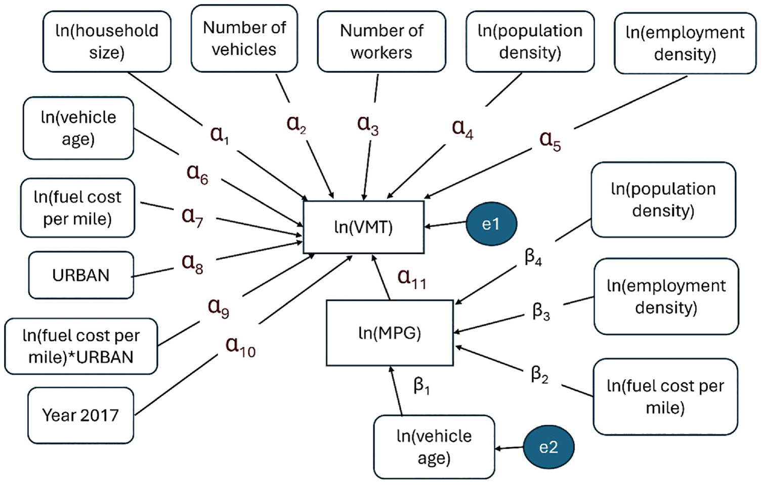
Structural equation system.
The model also had two unobserved error components, e1 and e2, that accounted for the variance in the dependent variables to capture any unobserved attributes not explained by the model. This included the impact of variables that were omitted from the model, but might still affect the output. The regression equations for all the states were as in Equations 3 and 4,
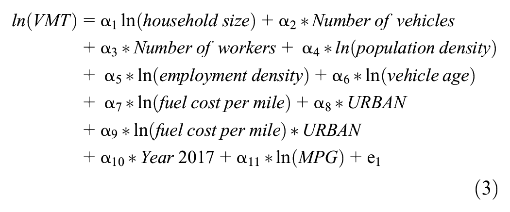
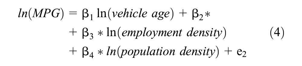
where
VMT = annual VMT in a household,
Household size = number of members in a household,
Number of vehicles = number of surveyed vehicles in a household,
Number of workers = number of workers in a household,
population density = population density of the census tract where the household is located,
employment density = household annual income,
vehicle age = average age of vehicles in a household,
fuel cost per mile = fuel cost per mile ($/mi),
MPG = fuel efficiency (mpg), and
Year 2017 = dummy variable: for 2017 data, Year 2017 = 1; for 2009, Year 2017 = 0;
URBAN = dummy variables: for urban areas, URBAN = 1; for rural areas, URBAN = 0.
The annualized fuel cost in U.S. dollars per gallon for each vehicle was obtained from the NHTS dataset. Fuel cost per mile was obtained by dividing the fuel cost by the associated fuel mpg. The mpg values used were obtained from NHTS data (derived from www.fueleconomy.gov) using the data from Energy Information Administration (EIA) based on the vehicle’s make, model, and year. If a household owned more than one vehicle, the cost per mile was weighted by the individual vehicles’ VMT and the weighted average of cost per mile was calculated using Equations 5 and 6.
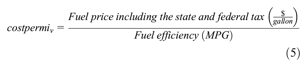

where
The VMT used in this equation was the self-reported annualized VMT for each household. Natural logarithms of each variable were taken, with the exception of the number of vehicles, number of workers, and two dummy variables: Year 2017 and URBAN. The coefficient (
Regression Model Result
The regression model coefficients have been summarized in Tables 2 to 5 for CA, IA, NY, and TX respectively. The sample sizes for each category of income classes were reasonably well above the critical sample size of 200 for providing sufficient statistical power of analysis ( 33 ). These models had comparative fit indices that were higher than 0.90, indicating that more than 90% of the covariation in the data could be reproduced by the given models (>0.90 implies good fit) ( 32 ). Chi-square (χ2) values of all the models were significantly greater than the cut-off value (35.60) at the 0.05 level with 51 degrees of freedom. The other goodness-of-fit measurements of the models (i.e., adjusted R-square and root mean square error of approximation [RMSEA]) are given in Tables 2 to 5. Although the RMSEA values were higher than the acceptable cut-off points of 0.08 for a good fit, acceptable values depend on model complexity, specific research context, and sample sizes.
Regression Model Result and Model Fit for California
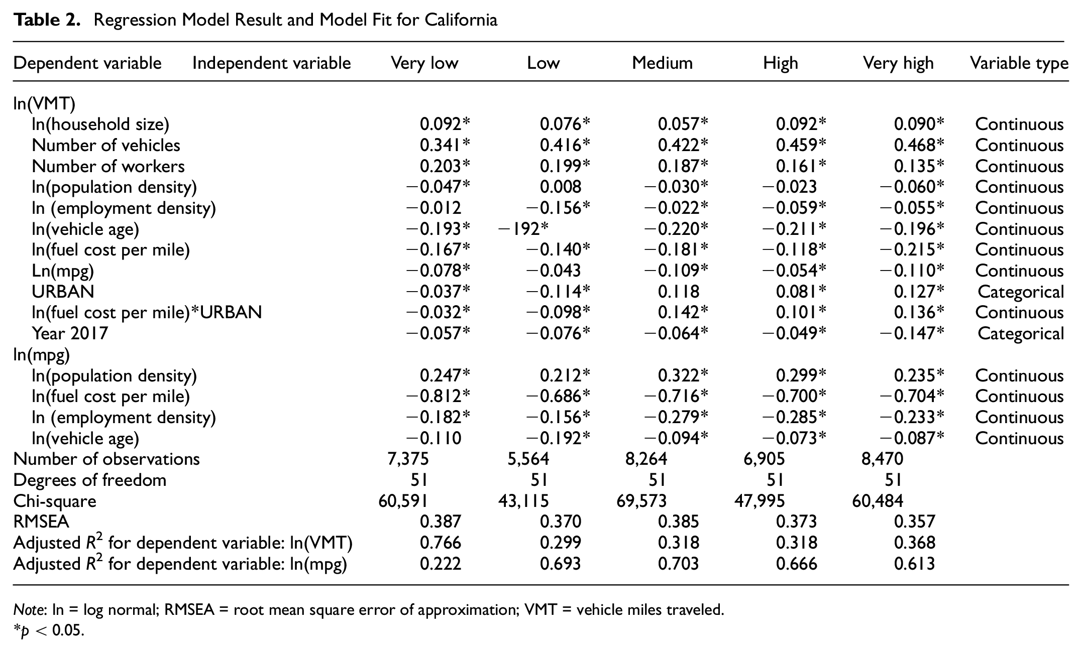
Note: ln = log normal; RMSEA = root mean square error of approximation; VMT = vehicle miles traveled.
p < 0.05.
Regression Model Result and Model Fit for Iowa
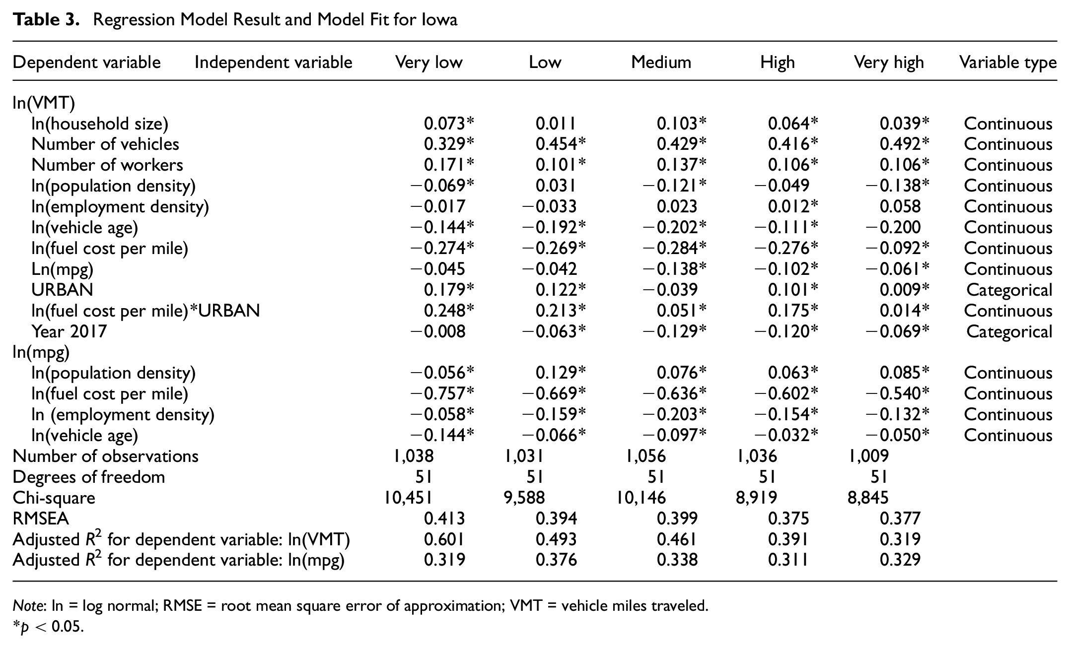
Note: ln = log normal; RMSE = root mean square error of approximation; VMT = vehicle miles traveled.
p < 0.05.
Regression Model Result and Model Fit for New York
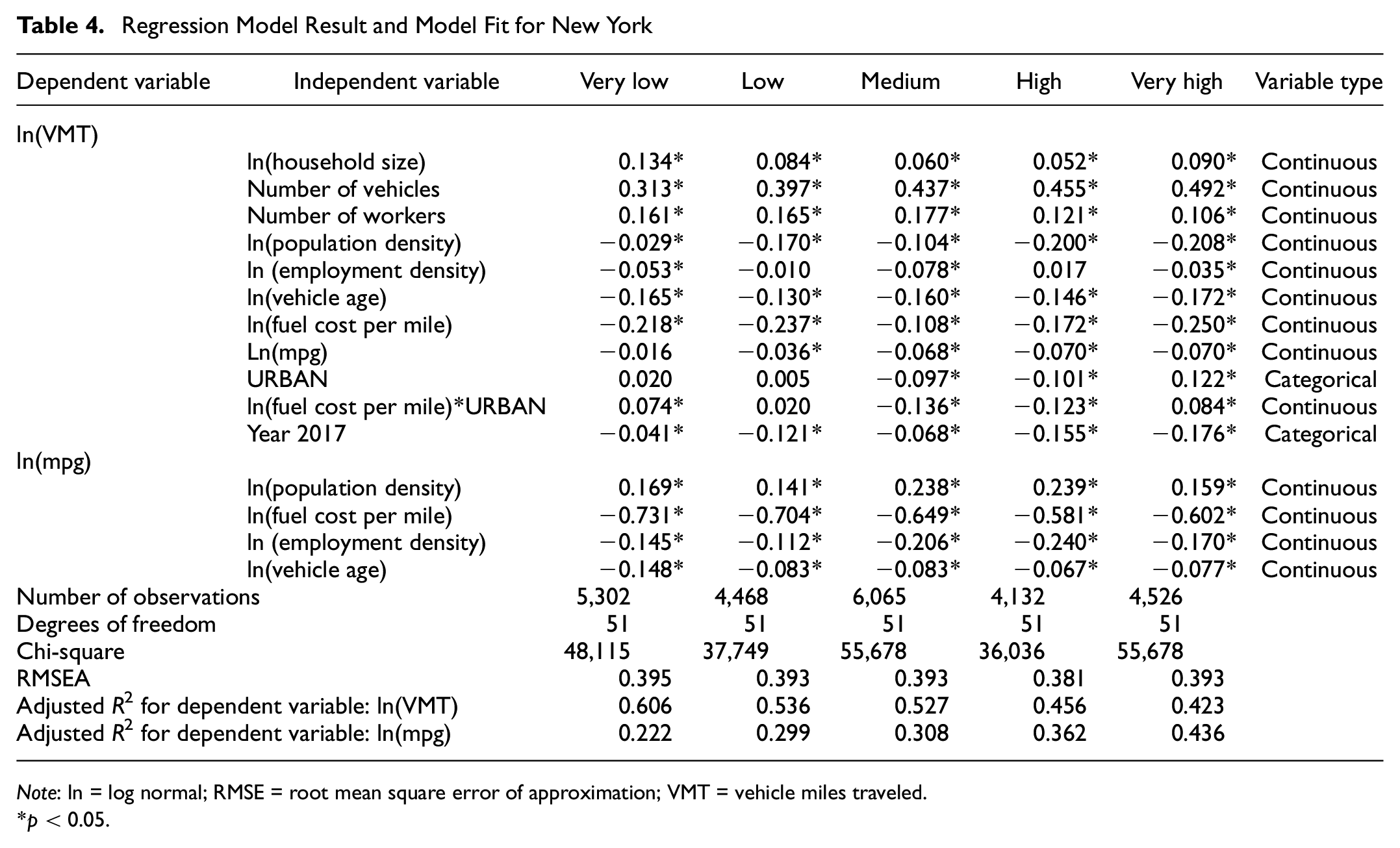
Note: ln = log normal; RMSE = root mean square error of approximation; VMT = vehicle miles traveled.
p < 0.05.
Regression Model Result and Model Fit for Texas
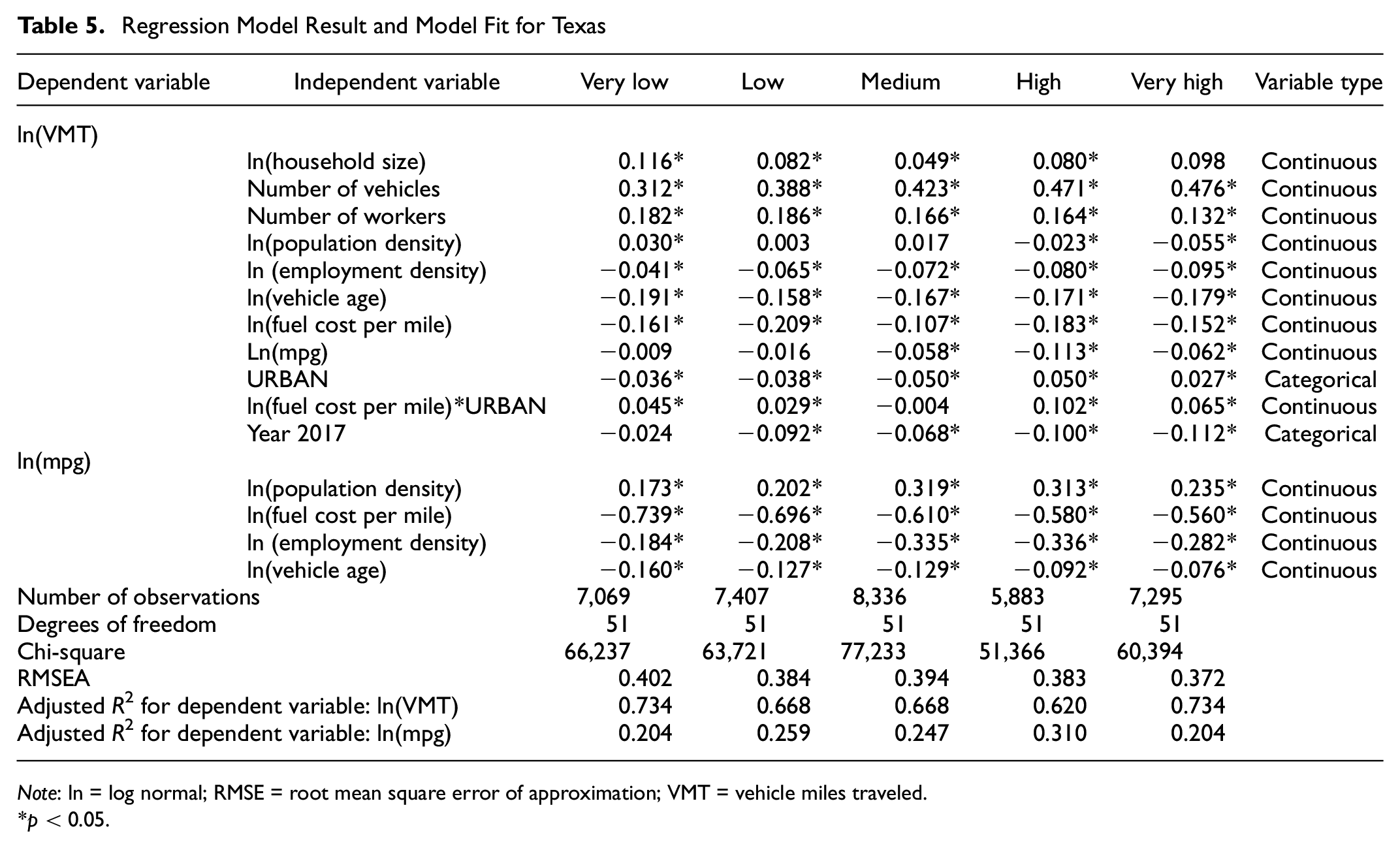
Note: ln = log normal; RMSE = root mean square error of approximation; VMT = vehicle miles traveled.
p < 0.05.
The signs of the coefficients for most of the variables indicated reasonable interpretations and were consistent with our expectations. As anticipated, the price of gasoline had a negative correlation with VMT: as the price of fuel rises, people tend to reduce the miles driven to save on cost. The number of workers, number of vehicles, and household size (number of members in a household) were all positively correlated with VMT for all the states. The coefficients of population density and employment density were mostly negative, which could indicate that in denser areas (i.e., more urban), people tend to drive less because of traffic congestion and shorter commute distances to workplaces and other amenities. The positive coefficient of population density with the dependent variable mpg indicated that households in densely populated areas had a higher probability of driving fuel-efficient vehicles, which is consistent with the findings from previous studies ( 34 ). The negative association between vehicle age and fuel efficiency indicated that older vehicles tended to have lower mpg, consistent with advancements in vehicle technology over time. The strong negative association (−0.581 to −0.731) between fuel cost per mile and fuel mpg across the states and income groups suggests that higher fuel costs are associated with lower observed mpg in the short term because rising fuel prices per mile are associated with lower mpg as the low fuel-efficient vehicles consume more fuel per mile. In the short run, the cost and practical constraints associated with replacing a vehicle may limit the immediate adoption of more efficient vehicles, despite rising fuel costs.
Elasticity of VMT Model Results
Elasticity from the Structural Equation Model
The purpose of the elasticity calculation was to understand the travel behavior under the new tax policy. Table 6 provides a summary of the elasticity results from structural equation models.
Elasticity results from OLS Model
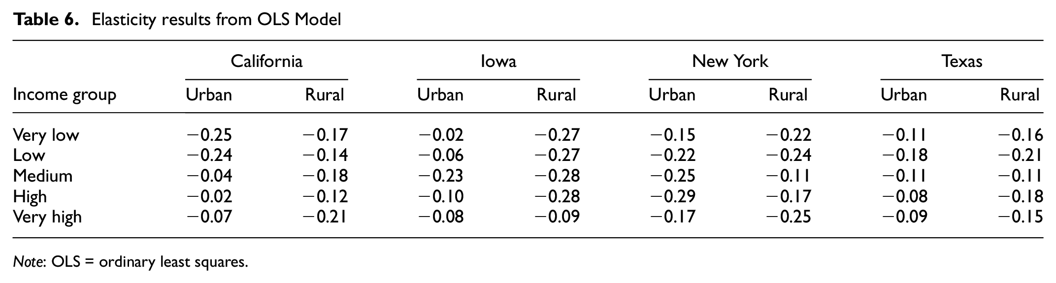
Note: OLS = ordinary least squares.
Price elasticities of VMT demand were all negative, as expected, ranged between −0.02 and −0.29, and were statistically significant for all income quintiles at the 0.05 level. Across income groups, the elasticity did not consistently increase or decrease with income. However, a common trend was that the elasticities of medium- to high-income groups were usually lower compared with very low- and low-income groups. In addition, it is important to recognize that these elasticity estimates primarily reflect short-run elasticities resulting from consumer responses. As such, they do not capture the potential long-term adjustments people make, such as changes in vehicle ownership, relocation of residences and workplaces, or the decision to telework. Comparing these findings with existing literature, Alberini et al. identified a price elasticity range of −0.2 to −0.275 ( 35 ), whereas Goetzke and Vance observed values typically below −0.1, yet occasionally reaching up to −0.4 ( 28 ). There were no studies that explicitly showed the difference in elasticities between urban and rural areas. However, Wenzel found an elasticity of −0.09 and indicated that lower-income and lower-density regions experience larger VMT reductions with increasing gas prices ( 36 ). Interestingly, despite fewer alternative transportation options, low-density regions (rural areas) saw the greatest decrease in VMT, which is consistent with our findings.
Scenarios
Three scenarios were examined in the study (see Table 7): all examined the annual household tax burden based on the household’s location (urban or rural) and income group. The scenarios differed based on the tax system and VMT fee rate. Unfortunately, the 2017 NHTS data grouped EVs, hybrid vehicles, and alternative fuel vehicles in one category. In our study, all those vehicles were counted as EVs.
Scenarios Examined
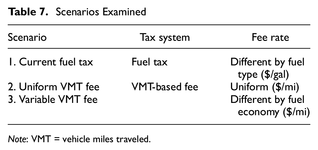
Note: VMT = vehicle miles traveled.
In the first scenario, the distribution of the current state fuel tax burden was examined. Under the current fuel tax system, the tax rate differed by fuel type. Therefore, the fuel tax was imposed on gasoline and diesel vehicles as described in the fuel tax section above. Since EVs do not pay fuel tax under the current fuel tax system, EVs were excluded from the first scenario. In the second scenario, a uniform VMT-based fee was imposed by each state. Because the VMT fee was set to collect the same amount of revenue as the current fuel tax, the rate was different in each state. This rate was imposed on all types of vehicle, regardless of the fuel type or fuel economy under the second scenario. In the third scenario, the VMT fee was again set to produce the same revenue as the state fuel tax, but the rate varied according to each vehicle’s fuel economy. Vehicles with better fuel economy had a lower VMT fee rate as an encouragement for people to select fuel-efficient vehicles. In each state, vehicles were split into three groups based on fuel economy: the highest, middle, and the lowest fuel economy group each included one-third of vehicles in each state. The basic level of VMT fee rate was applied to the middle level fuel economy group, whereas 0.4 cents per mile was added to the lowest fuel economy group and 0.4 cents per mile was subtracted for the highest fuel economy vehicles. The different settings of Scenarios 1, 2, and 3 are summarized in Table 7. EVs paid the same VMT fee rate as other vehicles in Scenario 2. In Scenario 3, EVs paid the lowest VMT fee rate, which was applied to the highest fuel economy group of gas-powered vehicles.
Impact of the VMT Fee
Current Fuel Tax
In the first scenario, the current state fuel tax paid by each household was calculated using Equation 7. The current fuel tax was imposed on the amount of fuel consumed by all vehicles in each household. This fuel consumption was calculated based on the annual VMT and the fuel economy information of each vehicle in each household. Another factor was the fuel tax level, which was different according to fuel type and state. When a household had several vehicle types, the fuel economy of each vehicle was applied to calculate the fuel consumption, and the fuel type was considered when applying the tax rate.
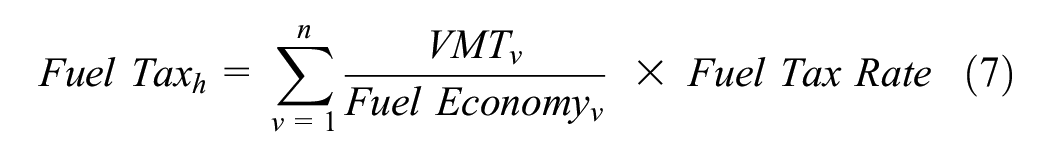
where
Fuel Tax Rate = fuel tax rate different by fuel type, state,and year ($/gal); and
Fuel Economy v = fuel economy of vehicle, v, (mi/gal).
The fuel tax of individual households was aggregated by income group (i), regional group (r), and state (s). Finally, the average fuel tax paid by a household that belongs to income group i, regional group, r, in state, s, was calculated using Equation 8 for the first scenario.
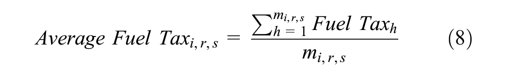
where Average Fuel Tax i,r,s is fuel tax paid by a household in an income group, i, region, r, in state, s ($/household/year); and m i,r,s is number of households that belong to income group, i, in region, r, in state, s. Households with only EVs were excluded from the gas tax scenario, but included in the VMT fee scenario.
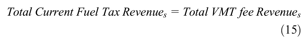
The total tax revenue under each VMT fee scenario (Scenarios 2 and 3) was set to equal the amount of state fuel tax collected by the current state fuel tax. The level of the VMT fee was set to meet this condition. For example, the level of the VMT fee under Scenario 2 was set through Equation 9.

where VMT fee s is level of VMT fee set in the state, s ($/mi), and ms is number of households in state, s.
Under Scenarios 2 and 3, VMT was assumed to change in line with the change in the travel cost. This reaction was estimated by applying the price elasticity of VMT estimated in the previous section. The changed VMT of each vehicle (
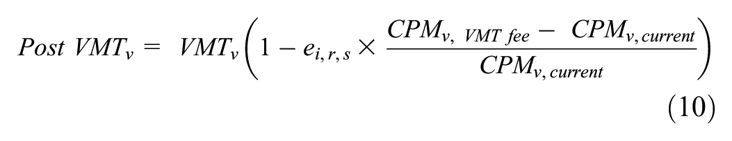
where
Post VMTv is VMT of a vehicle v after the application of VMT fee;
ei,r,s is price elasticity of a group belonging to income group, i, and regional group, r, in state, s;
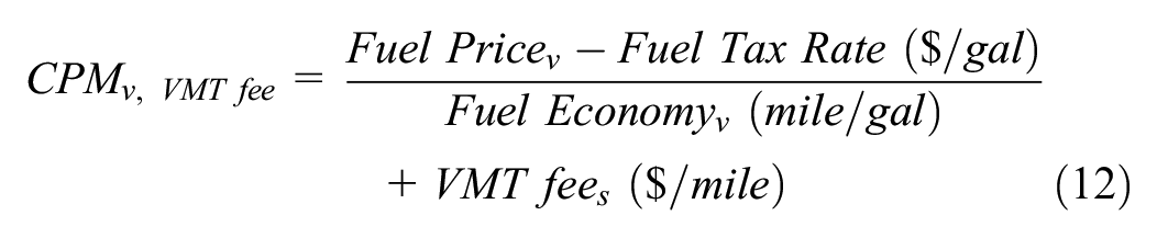
CPMv,VMT fee is cost per mile of vehicle, v, under the VMT fee system; and
CPMv, current is cost per mile of vehicle, v, under the current fuel tax system.

For Scenario 2, the VMT fee that would be paid by an individual household was calculated through Equation 13. Then, the average VMT fee per household based on income group (i), regional group (r), and state (s) was calculated using


where VMT fee hs is VMT that will be paid by a household, h, in state, s ($/household/year); and Average VMT fee i,r,s is fuel tax paid by a household in income group, i, regional group, r, in the state, s ($/household/year).
For Scenario 3, the VMT fee was set differently based on the vehicles’ fuel economy. The
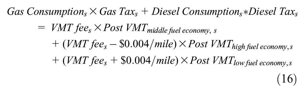
The implementation of a tiered VMT fee rate means that the fee is contingent on the fuel economy of each individual vehicle. Consequently, the variability in VMT fee rates among different income groups can be attributed to the diverse fuel economies of the vehicles within these groups. In Scenario 3, the average VMT fee rate was calculated and vehicles with average fuel economy (i.e., the middle-third of all vehicles) paid that average rate. For vehicles with worse fuel economy, the fee was 0.4 cents more. For vehicles with better fuel economy, the rate was 0.4 cents less. Table 8 shows the average VMT fee rates by income group utilized in Scenarios 2 and 3. Although different VMT fees based on the fuel economy level were applied, Table 8 shows its average value in each income group.
Vehicle Miles Traveled (VMT) Fee Rate
This table shows the VMT fee rate for vehicles with fuel economies in the middle third of all fuel economies in that state. In Scenario 3, for vehicles with worse fuel economy, the fee was 0.4 cents more. For vehicles with better fuel economy, the rate was 0.4 cents less.
Results and Analysis
Tax Burden by Scenario
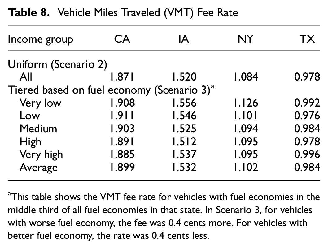
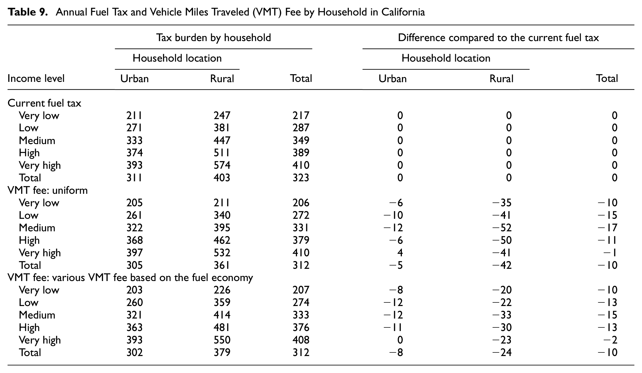
Based on the estimated elasticities in the previous section, the 2017 NHTS data, and the equations shown above, VMT fees paid by each household were estimated and then aggregated by group. Under the VMT fee scenarios, the same total tax revenue was collected as with the current state fuel tax scenario. The results are presented in Tables 9 to 12. Each table shows the analysis results by state and the relative difference between the VMT fee and the current state gas tax paid by the average household in that group. The average current fuel tax in a household was highest in CA ($323/household/year) followed by IA ($266/household/year), NY ($201/household/year), and TX ($194/household/year). This was a result of the different tax rates by state. As a reference, the VMT per household was highest in TX (19,672 mi/household/year), followed by NY (18,417 mi/household/year), IA (17,177 mi/household/year), and California (16,725 mi/household/year).
Annual Fuel Tax and Vehicle Miles Traveled (VMT) Fee by Household in California
Annual Fuel Tax and Vehicle Miles Traveled (VMT) Fee by Household in Iowa

Annual Fuel Tax and Vehicle Miles Traveled (VMT) Fee by Household in New York

Annual Fuel Tax and Vehicle Miles Traveled (VMT) Fee by Household in Texas
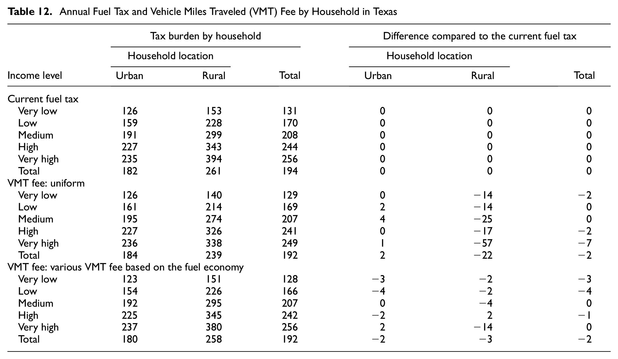
In all states, the tax burden of rural households was higher than that of urban households. In addition, higher-income groups’ tax level was higher than lower-income classes. Compared with the current fuel tax system, a household in CA paid $10 less in a year ($323 versus $312, as found in Table 9) whereas households in IA, NY, and TX paid $5, $2, and $2 less. This was because the current fuel tax was imposed on households who did not own EVs whereas the VMT fee system imposed fees on all households including those with EVs. The higher the proportion of EVs, the bigger the gap between the current fuel tax level and the VMT fee level. As a reference, the proportion of EVs was highest in CA (5.5%), followed by IA (2.8%), TX (2.2%), and NY (2.0%). With VMT fees, rural households still paid more than urban households, and higher-income groups paid more than lower-income groups, as in the current fuel tax system. However, both of those gaps narrowed, especially with rural households paying significantly less under several VMT fee scenarios than with the current state fuel tax system. This occurred because vehicles in rural households typically had lower fuel efficiency and traveled longer distances than vehicles from urban households, on average. Vehicles with lower fuel efficiency consume more fuel for the same distance traveled compared with those with higher efficiency, resulting in higher fuel taxes for owners of less efficient vehicles. Conversely, uniform VMT fee scenarios established a consistent fee for each mile traveled, regardless of fuel economy differences. Consequently, the tax burden on rural households decreased. With a tiered VMT fee system, under which less fuel-efficient vehicles face higher VMT fees, the reduction in tax burden among rural households was smaller than under the uniform VMT fee system. The impact of changes between urban and rural households on a per-household basis was greater for rural households since there were far fewer rural households over which to distribute any change in the tax burden.
This research also performed a similar analysis as above, but assuming there would be no change in VMT by vehicle from the new VMT fee. This is often referred to as a static scenario. The results were very close to the results of the dynamic scenario provided in Tables 9 to 12 and thus are not included in this paper.
Discussion
In this study, VMT fee scenarios were examined and compared with the current fuel tax level in four states—CA, IA, NY, and TX—using combined 2009 and 2017 NHTS data. The current average state fuel tax burden in each state was determined at the household level for different income and geographic groups. For the static scenario (i.e., travel behavior was assumed to be constant), VMT did not change. Under the dynamic scenario, the change in VMT resulting from the price change was determined using a structural equation elasticity model developed using NHTS data. VMT fee scenarios that collected the same amount of revenue as the current state fuel tax revenue were developed.
On average, a household in CA paid $10 less per year compared with the current fuel tax system. Households in IA, NY, and TX paid $5, $2, and $2 less, respectively, than the current fuel tax. This was because of EVs paying a VMT fee. In the current fuel tax system, rural households paid more than urban households on average, and higher-income groups paid more than lower-income groups on average. In the uniform VMT fee scenario, rural households experienced a larger decrease in the tax burden compared with urban households. This was partially because of the lower fuel economy of rural vehicles causing them to use more gas and pay more gas tax in the current system, and partially because of the smaller number of rural households over which any change was distributed. This result was similar to the results of the equity analysis conducted in a pilot project ( 37 ). Vehicles with lower fuel efficiency consume more fuel for the same distance traveled compared with those with higher efficiency. Consequently, owners of less fuel-efficient vehicles ended up paying more under a fuel tax system as compared to a VMT fee system. With a tiered VMT fee system, under which lower fuel efficiency vehicles face higher VMT fees, the reduction in the tax burden among rural households was not as large as under the uniform VMT fee, although some rural households still experienced more tax burden reduction than those in urban households. Overall, the tax burden will be more evenly distributed for the average household under both the uniform and tiered VMT fee system compared with the current tax system.
However, it is important to note that the study assumed a revenue-neutral scenario in which total tax revenue collected under the VMT fee system matched that of the current fuel tax. Although the fuel tax has relatively low collection costs, the administrative costs of collecting VMT fees could be higher depending on the collection method, which may require setting higher VMT fee rates to maintain revenue neutrality. Our study did not account for the transaction costs or any revenue leakage. Future research should consider these factors as they will affect the VMT fee rates and possibly the resulting behavioral responses.
The VMT fee systems examined here improved the equity of the system by reducing the average differences in fuel taxes paid between low- and high-income households, and between rural and urban households under the current fuel tax system. This may not be considered a positive outcome as, under the VMT system, the decrease in amount paid was generally larger for higher-income households. This decreases the gap in the amount paid by high- and low-income households but also creates potential equity concerns since the benefit is greater for high-income households. However, the main point is that for most households the difference in the amount paid under the current state fuel tax system versus the VMT fee scenarios examined here was $10 or less per year. Thus, we found that a change to a VMT fee system would have only a small impact on equity. This study has showed some interesting variations in elasticity with respect to fuel prices, particularly the higher elasticities observed among rural residents. Given the lack of uniformity in these findings across different income groups and geographic regions, future research should explore the underlying causes of these differences. Investigating factors such as limited access to alternative transportation options, variations in vehicle type, and the acquisition of vehicles that are more fuel-efficient could provide some valuable understanding.
Footnotes
Author Contributions
The authors confirm contribution to the paper as follows: study conception and design: M. Rahman, H. Ju, M. Burris; data collection: M. Rahman, H. Ju; analysis and interpretation of results: M. Rahman, H. Ju; draft manuscript preparation: M. Rahman, H. Ju, M. Burris. All authors reviewed the results and approved the final version of the manuscript.
Declaration of Conflicting Interests
The authors declared no potential conflicts of interest with respect to the research, authorship, and/or publication of this article.
Funding
The authors received no financial support for the research, authorship, and/or publication of this article.