Sage Journals: Discover world-class research

Abstract

This paper documents and illustrates a practice-ready procedure for estimating changes in crash frequency for specific application circumstances for three intelligent transportation system treatments—Closed Circuit Television Cameras (CCTV), Dynamic Message Signs (DMS), and Road Weather Information Systems (RWIS). The procedure will allow an agency to directly evaluate the change in safety that may be associated with a contemplated treatment. In effect, the approach mimics the application of a Crash Modification Function (CMFunction) in that each potential application will, in principle, have its own Crash Modification Factor (CMF). The procedure uses an empirical Bayes framework with safety performance functions (SPFs) for treatment and non-treatment reference sites. The paper also presents those SPFs, which were developed from Pennsylvania freeway data. In principle, this cross-sectional approach can be applied, as it has been, for other safety treatments where safety effects vary with application circumstance and where that variability cannot be captured with conventional before–after studies.

Keywords

intelligent transportation systems freeways safety performance and analysis Bayesian methods crash modification factors (CMFs)crash prediction models

Intelligent transportation systems (ITS) are a significant component of the operations of state departments of transportation (DOTs) and are increasingly used to improve roadway operations. Understanding the safety implications of ITS can help secure funding for ITS. Many ITS applications are useful in managing traffic and improving response to incidents, and therefore could be expected to reduce the frequency and severity of crashes. However, there are currently very few studies that have developed high-quality crash modification factors (CMFs) for ITS applications. Knowing the safety implications of specific ITS treatments can help agencies implement these treatments for safety reasons in addition to operations purposes.

This paper addresses a need for estimating changes in crash frequency for specific application circumstances for three ITS treatments—closed circuit television cameras (CCTV), dynamic message signs (DMS), and road weather information systems (RWIS). This introduction establishes that need in first summarizing the pertinent details of these treatments and related existing knowledge on their safety effects. In so doing, it is recognized that these systems are not safety treatments, per se. In reality, there is range of ways in which they are used by agencies to make a variety of decisions that could indirectly affect safety performance.

CCTV are the cameras used to monitor traffic activity on major roadways. They are typically included as a method of collecting field data for traffic analysis and can be used as a component to monitor traffic in traffic monitoring stations. Depending on the agency, the cameras can be used for different purposes, including viewing roadway incidents/crashes or measuring speed and traffic composition. The main motivation for installing and using CCTV is for traffic management and to reduce congestion. CCTV are typically used for traffic observation, traffic incident or event verification, weather verification, traveler information, field device verification, and intelligent work zones ( 1 ). As a result, there are no studies or CMFs that have determined the safety impact of CCTV in the context of change in crashes.

DMS, also called variable message signs or changeable message signs, are electronic signs that are placed along or above major highways to deliver a wide range of information to drivers through changeable messages. The Manual on Uniform Traffic Control Devices ( 2 ) limits the use of DMS to display specific types of messages. Many studies investigated driver reactions to DMS but did not examine safety performance or produce CMFs (see, for example, Shealy et al. [ 3 ]). A literature review conducted for this research did include studies that examined the effect of DMS on speed, but the primary focus was crash-based studies that examined safety performance ( 4 – 8 ). Some of the studies were naïve before–after evaluations and did not adequately address many possible sources of bias, including regression-to-the mean, changes in traffic volume, and trends in the system. Overall, those studies provided mixed results, with some analyses showing a decrease in crashes when DMS are used, whereas other studies showed an increase in crashes.

RWIS efficiently process weather data and condense these data into an actionable format to support decision-making. Often managed at the State level, an RWIS comprises environmental sensor stations (ESS), a communications system, and a central data collection system. The ESS are placed in and near the roadway, though newer systems may also contain vehicle-based mobile RWIS sensors. There are over 2,400 RWIS ESS owned by State transportation agencies across the U.S., with at least one ESS in forty-nine States and Washington, DC ( 9 ). A 2019 survey of thirty-nine State DOTs found that 94% of agencies subscribe to RWIS data, and that the use of agency sensors such as RWIS has remained generally consistent over the past 10 years ( 10 ). Most safety research involving RWIS employs data collected through the system to study the effects of weather and road surface conditions on safety performance. Thus, the CMF Clearinghouse does not contain any CMFs for RWIS. However, a handful of studies have attempted to evaluate the safety effects of the RWIS itself. For example, El Esawey et al. performed a thorough evaluation of the safety benefits of using RWIS coupled with DMS on rural highways in British Columbia, Canada ( 11 ). The study analyzed data from six different locations where the DMS systems were in place and used an empirical Bayes (EB) study design ( 12 ) with three to four winter seasons of before data and three to six winter seasons of after data, depending on the location. The results showed a 32% reduction in winter fatal and injury crashes, which was statistically significant at a 95% confidence level.

Given the dearth of knowledge about the safety effects of the three ITS treatments and a need by agencies to estimate the changes in safety of specific applications, the research for this paper was aimed at developing, documenting, and illustrating a practice-ready procedure for addressing that need. Early in the research, it was revealed that conducting a robust before–after study would be an insurmountable challenge, given paucity of required data and the need for the results to reflect the reality that the safety effects of these treatments will vary with application circumstance. Therefore, it was decided to pursue a cross-sectional regression-type approach using data from treatment and non-treatment groups, recognizing the potential issues with this study design; these include inappropriate functional form, omitted variable bias, or correlation of variables that could lead to counterintuitive results in comparing the crash experience of two groups of sites or in making inferences about the safety effects of a variable ( 13 ).

Methodology

Overview

In pursuing a cross-sectional regression-type approach it was natural to first consider a more traditional approach of combining treatment and non-treatment groups and including an indicator variable for the treatment, and interaction terms between the treatment indicator and other site characteristics. However, the available data were not nearly extensive enough for such an approach. It was then decided to pursue an approach based on a procedure that was first developed and validated for estimating the expected changes in safety for a contemplated traffic signal installation ( 14 ). The procedure was later proposed and illustrated for roundabout installation ( 15 ).

The principle of the adopted procedure is as follows. Separate safety performance functions (SPFs) were estimated for sites with and without each of the three ITS treatments as a function of exposure and a set of other independent variables. Consistent with the Highway Safety Manual (HSM) ( 16 ) method for estimating the expected safety benefit of a planned countermeasure, the procedure is applied in concert with the EB methodology ( 12 ) if, as is likely the case, a crash history is available as a specific application circumstance. For untreated reference sites with higher-than-expected crash frequency, which are the sites that would typically get considered for a safety treatment, the EB method in essence will refine (increase) the SPF expected crash frequency to account for risk factors not included in the SPF. In so doing, it will estimate a safety benefit that is larger than that obtained by comparing predictions from the two sets of SPFs for treatment and non-treatment sites.

The EB methodology is used with the crash data for a recent period at a potential treatment site and the SPF prediction for the site to estimate the expected number of total and fatal plus injury (FI) crashes that would have occurred in the after period without treatment. The EB estimate for property damage only (PDO) crashes is then derived as the EB estimate for total crashes minus the EB estimate for FI crashes.

The appropriate treatment site SPF is then used to estimate the expected number of total and FI crashes that would occur if the treatment were implemented. The estimate for PDO crashes is then derived as the SPF estimate for total crashes minus the SPF estimate for FI crashes. The expected change in safety for a potential application of the treatment is the difference between the EB estimate and the treatment site SPF prediction.

Methodological Steps

An analyst may apply the procedure using the following steps, which are adapted from documentation in Kopitch and Saphores ( 8 ).

Step 1

Assemble appropriate SPFs (shown later) for equivalent non-treatment and treatment sites and the data required to apply the SPFs. For the past, say, 3–5 years, obtain the count of total and FI crashes, and for the same period obtain the annual average daily traffic (AADT) values. Estimate the AADTs that would prevail for the period after the treatment is installed,

- If the SPFs cannot be assumed to be representative of the jurisdiction, they must be calibrated using data from a sample of sites representative of that jurisdiction using the HSM calibration procedure.

Step 2

Use the EB methodology with the data from Step 1 and the SPF for non-treatment sites to estimate the expected number of total and FI crashes that would occur without treatment. The EB estimate for PDO crashes is then derived as the EB estimate for total crashes minus the EB estimate for FI crashes. The equations are as follows:

EB estimate (m) = w_{1} (x) + w_{2} (nP)

where

x = the count of crashes (total or FI) in n years

P = the SPF prediction for the given input data (total or FI crashes)

w₁, w₂ are weights estimated as follows:

\begin{matrix} w_{1} = nP / (ȹ + nP) \\ w_{2} = ȹ / (ȹ + nP) \end{matrix}

where ф is the inverse overdispersion parameter estimated in the SPF calibration (these are presented later with the SPFs).

Step 3

Use the appropriate treatment site SPF and the AADTs from Step 1 to estimate the expected number of total and FI crashes that would occur if the treatment were implemented. The estimate for PDO crashes is then derived as the SPF estimate for total crashes minus the SPF estimate for FI crashes.

Step 4

Obtain for FI and PDO crashes, the difference between the estimates from Steps 2 and 3.

Step 5

Applying suitable severity weights and dollar values for FI and PDO crashes, obtain the estimated expected economic benefit of implementing the treatment.

Data

Datasets for estimating the SPFs were assembled for sites in Pennsylvania with the three treatments and for untreated reference sites for each. Unusable or unrealistic segments, such as segments with unrealistic AADT values or number of lanes, were filtered out. It was necessary to specify a buffer for the ITS treatments because they affect the surrounding area of a treatment location and not just the individual location. The research team identified a buffer around a specific treatment and assigned crashes in that buffer area to the ITS treatment for analysis. A 15 mi buffer was used for the DMS and RWIS treatments and a 1,500 ft buffer was used for CCTV treatments after preliminary analysis indicated that this afforded the best predictive ability for the SPFs developed. Summary statistics are provided in Tables 1 and 2. The research team was not able to access specific messages or general message categories displayed on the DMS at different times, so those data are not included in the summary statistics or the analysis. Note that the average AADTs for the treatment sites are higher than for the non-treatment sites, suggesting that the SPFs for treatment sites are likely more reliable for medium and higher AADTs than those for the non-treatment sites.

Table 1.

Number and Mileage of Sites and Proportion of Sites with Key Characteristics

Parameter	Treatment sites			Non-treatment sites
Parameter	CCTV	DMS	RWIS	CCTV	DMS	RWIS
Number of sites	31,318	122,068	106,039	28,353	9,378	25,407
Mileage	15,966	61,103	53,214	14,119	4,659	12,548
Proportion of sites
Lanes >2	0.44	0.19	0.18	0.20	0.07	0.18
Divisor width ≥11 ft	0.70	0.85	0.83	0.81	0.87	0.95
Speed limit ≥65 mph	0.14	na	na	0.40	na	na
Speed limit = 70 mph	na	0.22	0.24	na	0.27	0.19
Fixed barrier divisor	0.78	0.50	0.47	0.64	0.53	0.64
Urban sites	na	0.57	0.54	na	0.33	0.57

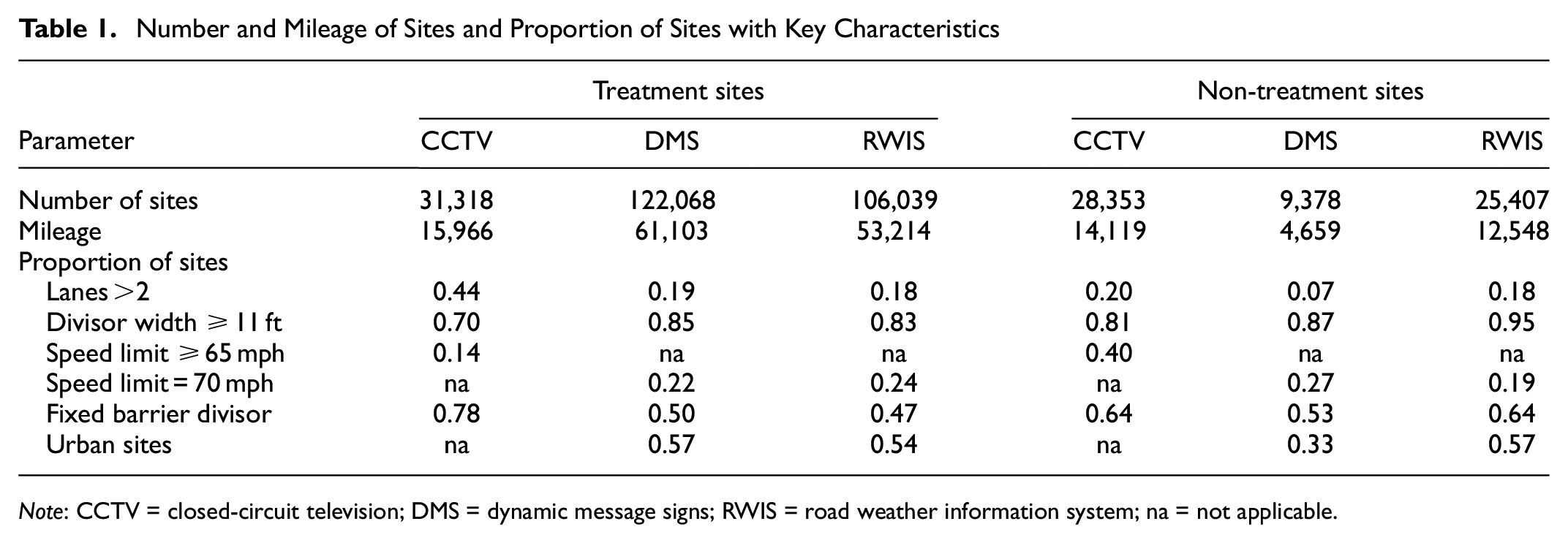
Note: CCTV = closed-circuit television; DMS = dynamic message signs; RWIS = road weather information system; na = not applicable.

Table 2.

Data ranges for AADT and Segment Length

Variable	CCTV		DMS		RWIS
Variable	Treatment	Reference	Treatment	Reference	Treatment	Reference
Min. AADT	3,500	3,500	127	44	127	3,948
Avg. AADT	34,813	23,270	25,152	16,979	23,317	19,075
Max. AADT	116,526	112,097	116,256	89,855	116,526	109,194
Min. Length (miles)	0.04	0.04	0.001	0.02	0.04	0.103
Avg. Length (miles)	0.5	0.4	0.5	0.525	0.5	0.49
Max. Length (miles)	1.2	1.2	1.2	1.09	1.2	0.733

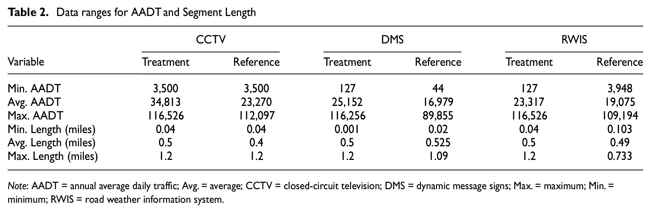
Note: AADT = annual average daily traffic; Avg. = average; CCTV = closed-circuit television; DMS = dynamic message signs; Max. = maximum; Min. = minimum; RWIS = road weather information system.

Safety Performance Functions (SPFS)

The following model form was used for estimating SPFs for treatment and non-treatment reference sites for each of the three treatments and for total and FI crashes:

Crashes / year = α L^{γ} {(AADT)}^{τ} e^{(β_{1} X_{1} + β_{2} X_{2} + β_{3} X_{3} + \dots .)}

where

L = segment length;

AADT = average annual daily traffic;

The Xs are segment characteristics.

α, τ, γ, and the βs are coefficients estimated from data in the regression analysis procedure.

Consistent with common practice, generalized linear modeling with a negative binomial (NB) error structure was used for model estimation, using the software R. An inverse overdispersion parameter of the NB distribution is also estimated in the model calibration process. As estimated with the R software, the larger the value of the inverse overdispersion parameter, the better the model is for the same estimation data.

Non-treatment reference sites were selected from similar locations where the given treatment had not been applied. The research team first used propensity score matching methods to better match the characteristics of treated and untreated sites, specifically in the case where there were fewer treatment sites than reference sites. This matching method first estimates propensity scores for each site, which is a probability between 0 or 1 that site will receive a treatment ( 17 ). For this study, propensity scores were calculated based on the following characteristics: AADT, segment length, total roadway width, divisor width, number of lanes, district, area type (e.g., urban or rural), speed limit, surface type, and if the site is on the National Highway System. After calculating propensity scores for each site, the treatment and non-treatment sites were matched based on a one-to-one nearest-neighbor approach, where each non-treatment site was match to a treatment site with the closest propensity score within 10% ( 17 ).

SPFs were then estimated for matched and unmatched data and the two sets of models compared. In the end, the SPFs with the unmatched data turned out to be superior based on goodness of fit measure and logic of the direction of effects for variables. This was likely because of the significantly reduced sample sizes for the matched data.

The estimated SPFs for the unmatched data summarized in Tables 1 and 2 are shown in Tables 3 –5. It should be stressed that these are predictive models and are not intended for inferring causation or for quantifying the safety effects of individual variables for the reasons outlined in the introduction. It is also important, as emphasized in the HSM ( 16 ), and as noted earlier, that the SPFs be calibrated for application in jurisdictions other than Pennsylvania using procedures documented in the HSM.

Table 3.

Parameter Estimates (and Standard Errors) for Safety Performance Functions for Sites with and without CCTV

Parameter	With CCTV		Without CCTV
Parameter	Total	FI	Total	FI
(Intercept)	−6.5088 (0.2658)	−8.694 (0.3047)	−8.2729 (0.2114)	−9.8788 (0.272)
log(AADT)	0.7296 (0.0255)	0.8456 (0.0292)	0.9019 (0.0205)	0.9637 (0.0262)
log(segment length in miles)	0.5382 (0.0515)	0.5514 (0.058)	0.5032 (0.0574)	0.4404 (0.0721)
Lanes >2	0.2176 (0.0245)	0.2655 (0.0272)	0.0737 (0.0235)	0.1592 (0.0286)
Plain reinforced concrete surface	−0.2528 (0.0301)	−0.2488 (0.0344)	−0.0544 (0.0225)	−0.088 (0.0284)
Divisor width ≥11 ft	−0.2367 (0.0258)	−0.2136 (0.0283)	−0.3472 (0.0246)	−0.3763 (0.0303)
Lane width >12 ft	0.1927 (0.0256)	0.2467 (0.028)	−0.1385 (0.0295)	−0.1321 (0.0362)
Fixed barrier	−0.1979 (0.0321)	−0.088 (0.0371)	−0.4946 (0.0206)	−0.4603 (0.0264)
Speed limit ≥65 mph	−0.3302 (0.0379)	−0.3915 (0.0458)	−0.1365 (0.0208)	−0.153 (0.027)
Inverse overdispersion	0.3608 (0.0049)	0.3628 0.0066)	0.4884 (0.0075)	0.4774 (0.012)

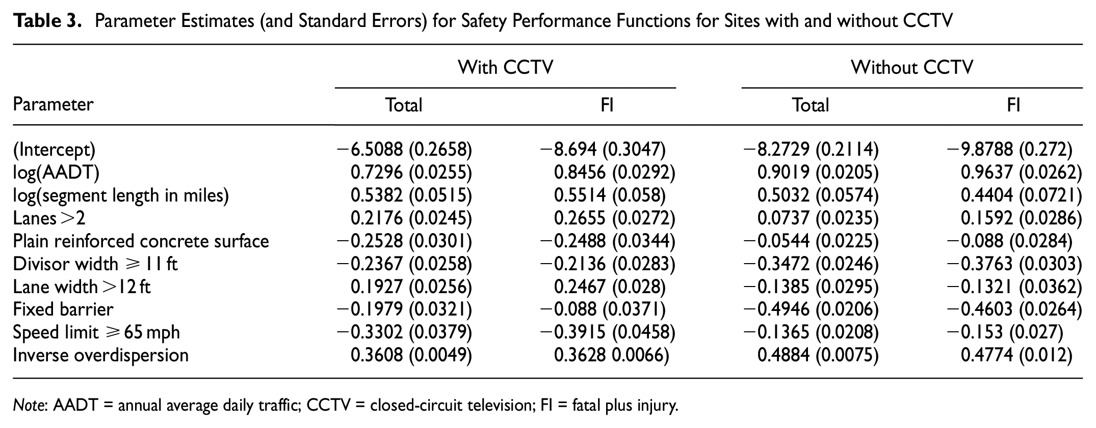
Note: AADT = annual average daily traffic; CCTV = closed-circuit television; FI = fatal plus injury.

Table 4.

Parameter Estimates (and Standard Errors) for Safety Performance Functions for Sites with and without DMS

Parameter	With DMS		Without DMS
Parameter	Total	FI	Total	FI
(Intercept)	−3.786 (0.2841)	−5.353 (0.3866)	−2.079 (0.4295)	−4.294 (0.5972)
Lanes >2	0.1364 (0.0155)	0.1987 (0.019)	na	na
Fixed barrier	−0.2168 (0.0148)	−0.17 (0.0192)	−0.285 (0.0199)	0.2676 (0.0276)
Divisor width ≥11 ft	−0.2198 (0.0165)	−0.218 (0.0202)
Non-bituminous surface	−0.0314 (0.0142)	−0.0604 (0.0182)	0.1347 (0.0273)	0.1735 (0.0379)
Bridge deck pavement	0.1775 (0.0302)	0.2419 (0.0359)	na	na
Speed limit = 70	0.0341 (0.0176)	na	0.1358 (0.0223)	na
Urban site	−4.644 (0.3582)	−4.318 (0.4799)	−1.807 (0.5043)	−2.248 (0.7393)
log(AADT) for rural sites	0.4451 (0.0299)	0.5024 (0.0405)	0.2205 (0.0477)	0.3504 (0.0664)
log(AADT) for urban sites	0.8884 (0.0377)	0.9098 (0.0485)	0.3738 (0.0731)	0.5483 (0.1052)
log(segment length in miles)for rural sites	0.8233 (0.082)	0.8602 (0.1184)	0.9013 (0.1018)	0.8155 (0.1494)
log(segment length in miles)for urban sites	0.5076 (0.0378)	0.5007 (0.0469)	0.6272 (0.1122)	0.5548 (0.1578)
Inverse overdispersion	0.5176 (0.0048)	0.4469 (0.0062)	0.8412 (0.0189)	0.6945 (0.0282)

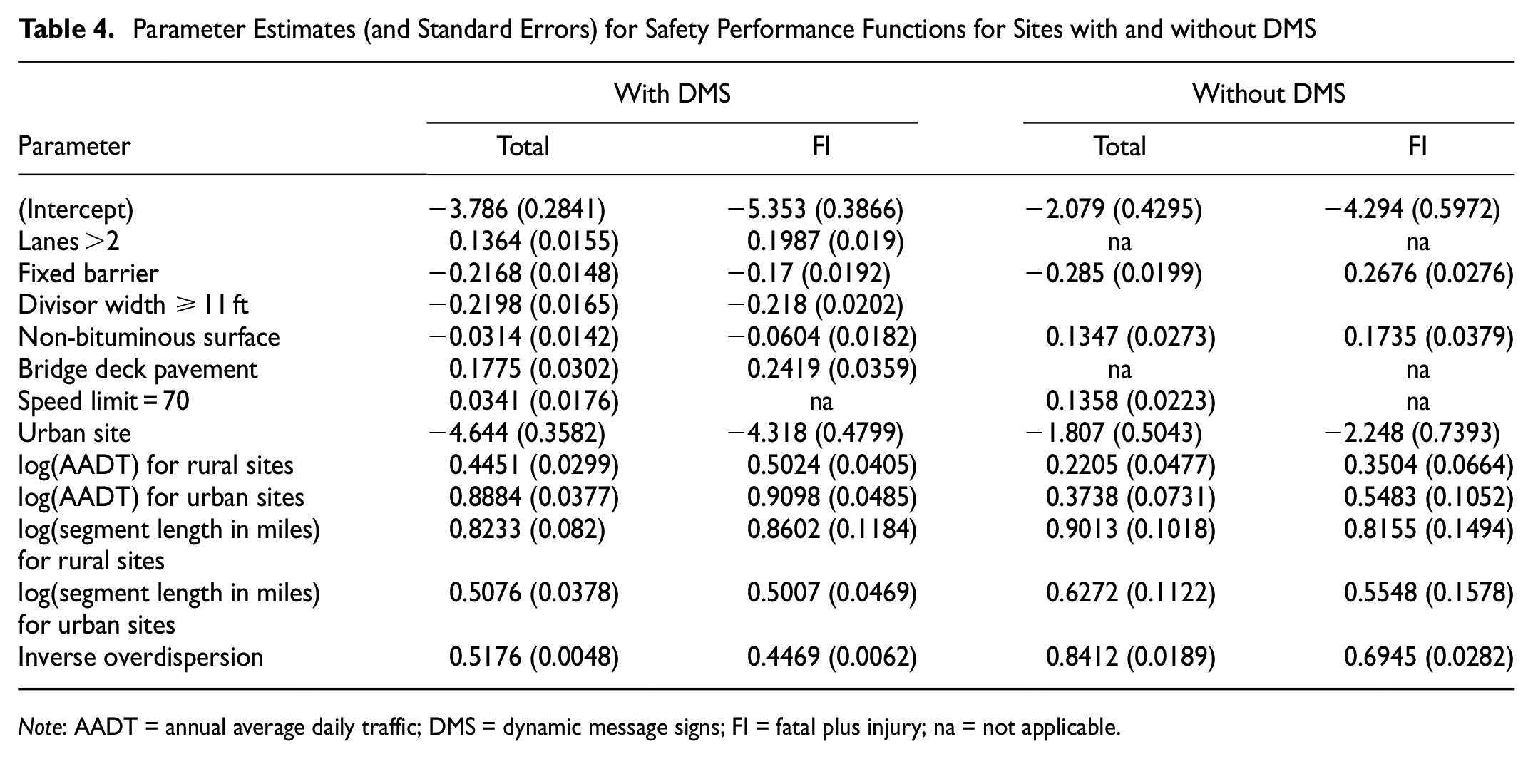
Note: AADT = annual average daily traffic; DMS = dynamic message signs; FI = fatal plus injury; na = not applicable.

Table 5.

Parameter Estimates (and Standard Errors) for Safety Performance Functions for Sites with and without RWIS

Parameter	With RWIS		Without RWIS
Parameter	Total	FI	Total	FI
(Intercept)	−4.118 (0.2363)	−5.8231 (0.3347)	−4.0437 (0.3903)	−6.8214 (0.5501)
Lanes > 2	0.1735 (0.0155)	0.2407 (0.0192)	na	na
Fixed barrier	−0.2089 (0.0141)	−0.155 (0.0186)	−0.2823 (0.0266)	−0.2701 (0.0361)
Divisor width ≥11 ft	−0.1676 (0.0156)	−0.1803 (0.0194)	−0.2035 (0.0545)	−0.1815 (0.0744)
Plain reinforced concrete surface	−0.0625 (0.0145)	−0.0857 (0.0191)	−0.1468 (0.0329)	−0.2286 (0.0431)
Speed limit = 70	0.0688 (0.0156)	0.0239 (0.0216)	0.171 (0.0317)	0.0819 (0.0445)
Urban site	−4.7854 (0.2708)	−5.0295 (0.3756)	−8.0525 (0.4669)	−8.9136 (0.6605)
log(AADT) for rural sites	0.4793 (0.0241)	0.5577 (0.0339)	0.4763 (0.0405)	0.6545 (0.0565)
log(AADT) for urban sites	0.9448 (0.014)	1.045 (0.0181)	1.2722 (0.0296)	1.5519 (0.0389)
log(segment length in miles)for rural sites	0.8984 (0.0787)	0.9463 (0.116)	na	0.6222 (0.1548)
log(segment length in miles)for urban sites	0.5655 (0.0364)	0.5832 (0.0454)	na	0.8704 (0.1579)
log(segment length in miles)	na	na	0.7477 (0.0783)	na
Inverse overdispersion	0.5418 (0.004)	0.454 (0.0063)	0.687 (0.0159)	0.6263 (0.0246)

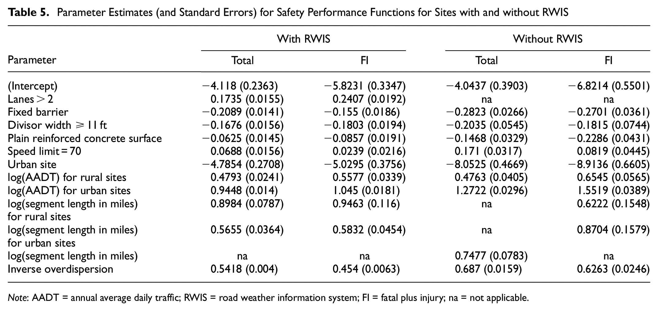
Note: AADT = annual average daily traffic; RWIS = road weather information system; FI = fatal plus injury; na = not applicable.

CMFs Derived from Illustrative Applications of the Proposed Procedure

For these illustrative applications, which are provided to demonstrate that the results from applying the procedure are reasonable, a freeway with three lanes in one direction (Lanes >2) is being considered for one of the three treatments. The following parameters pertain:

Segment length = 1.2 mi

Lane width = 12.5 ft

Speed limit = 70 mph

Fixed barrier; Divisor width = 15 ft

Surface type is plain Portland cement concrete base

Rural area

It is also assumed for convenience that the SPFs presented earlier may be applied without calibration. Table 6 shows the CMF derivation for two levels of AADT (medium and high) and assumed crash frequencies for 5 years before treatment that are assumed to be roughly proportional to those AADTs. AADTs are assumed to increase by 5% between the before and after period. The implied CMFs are estimated by dividing the crashes/year expected with treatment by the crashes/year expected without treatment.

Table 6.

CMFs Derived from Illustrative Applications of the Proposed Procedure

Treatment	AADT before	Crashes in most recent 5 years		Crashes/year expected without treatment		Crashes/year expected with treatment		Expected reductions in crashes per year with treatment		Implied CMF
Treatment	AADT before	Total	FI	PDO	FI	PDO	FI	PDO	FI	PDO	FI
CCTV	40,000	13	6	7.37	5.75	5.68	4.89	1.69	0.86	0.77	0.85
CCTV	90,000	25	11	14.61	11.11	9.39	9.71	5.22	1.40	0.64	0.87
DMS	40,000	13	6	7.07	5.51	6.65	4.54	0.42	0.98	0.94	0.82
DMS	90,000	25	11	13.78	10.11	9.23	6.82	4.55	3.29	0.67	0.67
RWIS	40,000	13	6	7.31	5.79	7.74	5.21	-0.44	0.59	1.06	0.90
RWIS	90,000	25	11	14.26	10.85	10.92	8.18	3.34	2.66	0.77	0.75

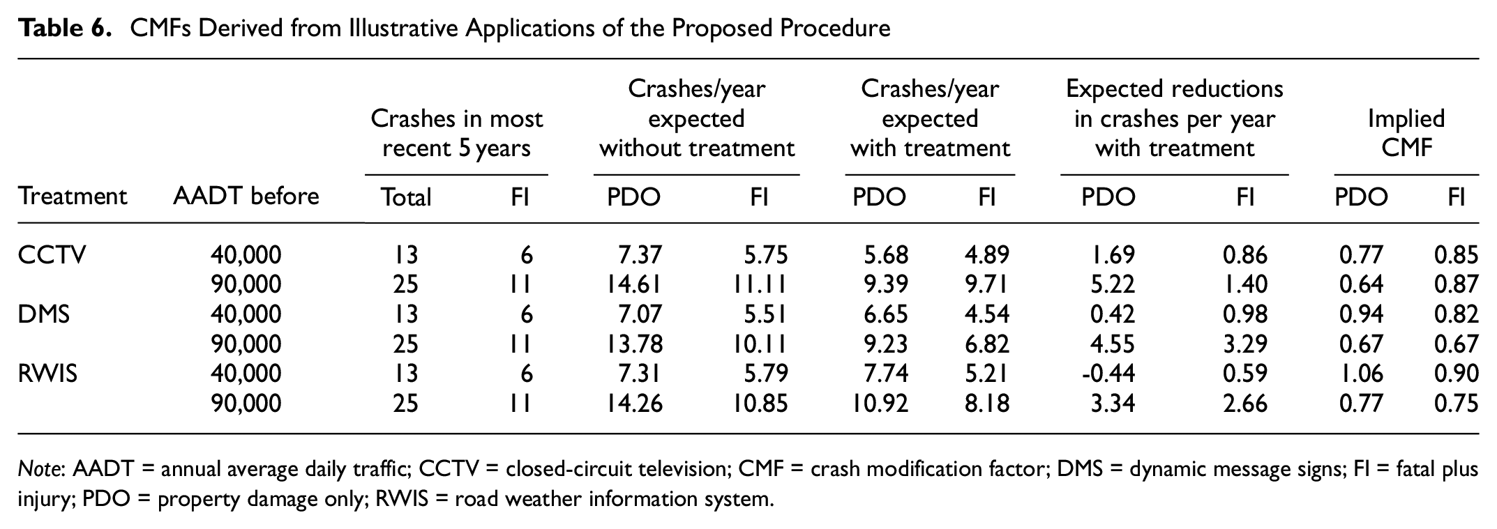
Note: AADT = annual average daily traffic; CCTV = closed-circuit television; CMF = crash modification factor; DMS = dynamic message signs; FI = fatal plus injury; PDO = property damage only; RWIS = road weather information system.

The following is an example calculation for CMFs in Table 6. It pertains to a three-lane site with AADT of 40,000 being considered for CCTV with an estimated AADT of 42,000 after implementation. The crash counts (x) in the past n = 5 years were: Total = 13; FI = 6.

For convenience of presentation, some steps from the methodological overview are combined, so the steps are given letters instead of numbers to avoid confusion. It is also assumed for convenience that the appropriate SPFs in Table 3 may be applied without calibration.

Step (a)

First, the SPFs for non-treatment sites are used to predict the number of crashes by severity based on the parameter estimates in Table 3 for the constant term, speed limit, surface type, lane count, lane width, presence of a fixed barrier, divisor width, AADT, and segment length.

Total crashes / year = P = e^{(- 8.2729 - 0.1365 - 0.0544 + 0.0737 - 0.1385 - 0.4946 - 0.3472)} \times 40, 000^{0.9019} \times 1 . 2^{0.5032} = 1.321

Inverse overdispersion parameter (ф) = 0.4884

FI crashes / year = P = e^{(- 9.87876 - 0.153 - 0.088 + 0.1592 - 0.1321 - 0.4603 - - 0.3763)} \times 40, 000^{0.9637} \times 1 . 2^{0.4404} = 0.529

Inverse overdispersion parameter (ф) = 0.4774

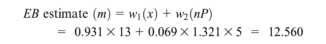
Next, the weights for the SPF prediction (P) and the crash counts (x) for the EB method, and the EB estimates are calculated. The SPF inverse overdispersion parameter (ф) is also used in these calculations.

Total crashes:

w_{1} = nP / (ȹ + nP) = 5 \times 1.321 / (0.4884 + 5 \times 1.321) = 0.931

w_{2} = ȹ / (ȹ + nP) = 0.4884 / (0.4884 + 5 \times 1.321) = 0.069

EB estimate (m) = w_{1} (x) + w_{2} (nP) = 0.931 \times 13 + 0.069 \times 1.321 \times 5 = 12.560

FI crashes:

w_{1} = nP / (ȹ + nP) = 5 * 0.529 / (0.4774 + 5 \times 0.529) = 0.847

w_{2} = ȹ / (ȹ + nP) = 0.4774 / (0.4774 + 5 \times 0.529) = 0.153

EB estimate (m) = w_{1} (x) + w_{2} (nP) = 0.847 \times 6 + 0.153 \times 0.529 \times 5 = 5.487

Because AADT is expected to increase in the after period, albeit only slightly, an adjustment is made to the EB estimate (m) to account for this change. This factor is calculated from the AADTs and their calibrated exponents as follows:

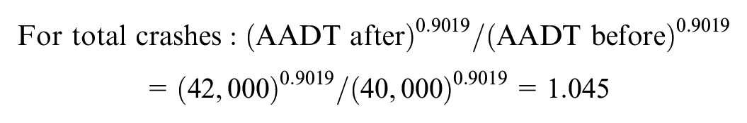
For total crashes : {(AADT after)}^{0.9019} / {(AADT before)}^{0.9019} = {(42, 000)}^{0.9019} / {(40, 000)}^{0.9019} = 1.045

The adjusted m is now equal to: 12.560 × 1.045 = 13.125 for total crashes.

For FI crashes:

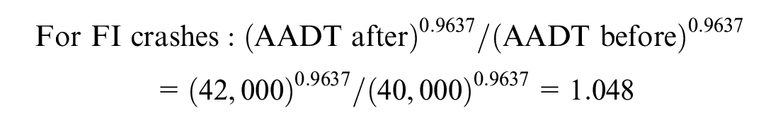
F o r F I c r a s h e s : {(A A D T a f t e r)}^{0.9637} / {(A A D T b e f o r e)}^{0.9637} = {(42, 000)}^{0.9637} / {(40, 000)}^{0.9637} = 1.048

The adjusted m is now equal to: 5.487 × 1.048 = 5.751 for FI crashes.

The expected number of crashes by severity at the site in future years if CCTV installation does not take place is estimated to be 13.125 total and 5.751 FI crashes, over a five-year period.

Step (b)

The treatment site SPF from Table 3 is used to predict the expected number of crashes should the CCTV be implemented. In this case, as noted, for convenience the SPF was deemed adequate and was not calibrated specifically for the jurisdiction. (Note: The future AADT is used in this calculation.)

Total crashes/year = e^{(-6.5088-0.3302-0.2528+0.2176+0.1927-0.1979-0.2367)} × 42,000^0.7296 × 1.2^0.5382 = 2.115. Over 5 years, this would be 2.115 × 5 = 10.574.

FI crashes/year = e^{(-8.6940-0.3915-0.2488+0.2655+0.2467-0.0880-0.2136)}\×42,000^0.8456×1.2^0.5514 = 0.979. Over 5 years, this would be 0.979×5 = 4.894.

The expected number of crashes by severity over 5 years at the site if CCTV were to be implemented is 10.574 total and 4.894 FI crashes.

Step (c)

The expected reduction in total crashes is equal to 13.125−10.574 = 2.551 crashes over 5 years.

The expected reduction in FI crashes is equal to 5.751−4.894 = 0.857 crashes over 5 years; the implied CMF is 4.894/5.751 = 0.85, shown in the first row of Table 6.

The expected reduction in PDO crashes is crashes 7.374−5.680 = 1.694 crashes over 5 years; the implied CMF is 5.680/7.374 = 0.77, shown in the first row of Table 6.

The CMFs in Table 6 illustrate the variability of CMFs with specific treatment application circumstances. One such CMF, for PDO crashes for RWIS for the lower AADT, indicates a potentially small increase in the minor crashes that is, in any case, compensated for by the larger decrease in the more severe FI crashes.

Conclusions

The research addressed a need identified in NCHRP Project 17-95 to develop CMFs for the various typically deployed ITS applications, DMS, CCTV, and RWIS. In so doing, the study provides an important contribution to the CMF knowledgebase by developing, documenting, and illustrating a procedure for estimating changes in crash frequency for specific application circumstances so that an agency can directly evaluate the change in safety that may be associated with a contemplated CCTV, DMS, or RWIS treatment. That procedure, which used an EB framework with SPFs for treatment and non-treatment reference sites, was developed and validated in previous research for evaluating the safety effects of traffic signal installation. Nevertheless, further validation for a wider range of site and treatment types would be useful and has been actually recommended as a research need by the TRB Safety Performance and Analysis Committee at the Transportation Research Board 2024 Annual Meeting.

Further research can also shore up the results from this project with the use of data from other jurisdictions to enhance the procedure developed for directly estimating the change in safety of a contemplated ITS treatment by testing its transferability and by increasing the robustness of the SPFs used in that procedure.

The procedure, as documented, is practice ready. However, potential users should be aware of caveats that result from some of its limitations. First, a fundamental assumption is that if a treatment that is evaluated with the procedure is implemented, then the site will have a safety experience with the treatment similar to equivalent ones used for the development of the treatment site SPFs. Second, the SPFs used in the procedure for treatment and non-treatment sites are intended for use in crash prediction with the EB methodology, so caution should be exercised in using them for comparison of the safety of the two site types. Finally, in accord with the HSM recommendations, the SPFs should desirably be calibrated for application in jurisdictions and time periods that are different from the ones for which there were developed.

Footnotes

Acknowledgements

Data for the research were provided by the Pennsylvania Department of Transportation. This research is part of the NCHRP Project 17-95, which is part of the National Cooperative Highway Research Program (NCHRP). NCHRP is administered by the Transportation Research Board (TRB) and funded by participating member states of the American Association of State Highway and Transportation Officials (AASHTO). NCHRP also receives critical technical support from the Federal Highway Administration (FHWA), United States Department of Transportation.

Author Contributions

The authors confirm contribution to the paper as follows: study conception and design: B. Persaud, R Srinivasan, V. Gayah; data collection: K. Kersavage, V. Gayah, R. Srinivasan; analysis and interpretation of results: V. Gayah, K. Kersavage, R. Srinivasan, B. Persaud, S. Hallmark, T. Saleem, C. Mohammadi; draft manuscript preparation: B. Persaud, R. Srinivasan, V. Gayah, K. Kersavage, S. Hallmark, T. Saleem, C. Mohammadi. All authors reviewed the results and approved the final version of the manuscript.

Declaration of Conflicting Interests

The author(s) declared no potential conflicts of interest with respect to the research, authorship, and/or publication of this article.

Funding

The author(s) disclosed receipt of the following financial support for the research, authorship, and/or publication of this article: Research funding was provided by the National Cooperative Highway Research Program (NCHRP) Project 17–95.

ORCID iDs

Bhagwant Persaud

Raghavan Srinivasan

Vikash Gayah

Kristin Kersavage

Taha Saleem

Shauna Hallmark

References

Balke

Chaudhary

Brydia

Songchitruksa

Pesti

Warrants and Criteria for Installing and Sunsetting TXDOT ITS Equipment. Report 0-6773-1. Texas Department of Transportation, Austin, 2014.

Federal Highway Administration. Manual on Uniform Traffic Control Devices for Streets and Highways. Department of Transportation, Washington, D.C., 2009.

Shealy

Kryschtal

Franczek

Katz

Driver Response to Dynamic Message Sign Safety Campaign Messages. Report No. FHWA/VTRC 20-R16. Virginia Department of Transportation and Federal Highway Administration, Richmond, 2020.

Tribbett

McGowen

Mounce

An Evaluation of Dynamic Curve Warning Systems in the Sacramento River Canyon. Western Transportation Institute, Bozeman, 2000. https://westerntransportationinstitute.org/wp-content/uploads/2016/08/429861_Final_Report.pdf.

Erke

Gottlieb

Psychologische Untersuchung der Wirksamkeitvon Wechselverkehrszeichenanlagen (Psychological Investigation of the Effectiveness of Traffic Sign Systems). Bundesministerium Fuer Verkehr, Bau und Wohnungswesen, 1980. https://trid.trb.org/view/1039066.

Cooper

Sawyer

Rutley

Analysis of Accidents Before and After Implementation of Improved Motorway Signalling. Transport Research Library, Wokingham, Berkshire, 1992. https://trid.trb.org/view/493301.

Persaud

Mucsi

Ugge

Safety Evaluation of Freeway Traffic Management System in Toronto, Canada. Transportation Research Record: Journal of the Transportation Research Board, 1996. 1553: 110–114.

Kopitch

Saphores

Assessing Effectiveness of Changeable Message Signs on Secondary Crashes. Presented at 90th Annual meeting of the Transportation Research Board, Washington, D.C., 2011.

Federal Highway Administration. Surveillance, Monitoring, and Prediction. Department of Transportation, Washington, D.C., 2017. https://ops.fhwa.dot.gov/weather/mitigating_impacts/surveillance.htm.

10.

Gopalakrishna

Gestwick

Road Weather Management and Performance Measures Update. Report FHWA-HOP-19-089. United States Federal Highway Administration, Washington, D.C., 2019.

11.

El Esawey

Walker

Sowers

Sengupta

Safety Assessment of the Integration of Road Weather Information Systems and Variable Message Signs in British Columbia. Transportation Research Record: Journal of the Transportation Research Board, 2019. 2673: 305–313.

12.

Hauer

Observational Before-After Studies in Road Safety: Estimating the Effect of Highway and Traffic Engineering Measures on Road Safety. Elsevier Science Incorporated, Tarrytown, NY, 1997.

13.

Gross

Persaud

Lyon

A Guide to Developing Quality Crash Modification Factors. Report FHWA-SA-10-032. Federal Highway Administration, Washington, D.C., 2010.

14.

Persaud

McGee

Lyon

Lord

Development of a Procedure for Estimating the Expected Safety Effects of a Contemplated Traffic Signal Installation. Transportation Research Record: Journal of the Transportation Research Board, 2003. 1840: 96–103.

15.

Rodegerdts

Bansen

Tiesler

Knudsen

Myers

Johnson

Moule

, et al. Roundabouts: An Informational Guide, 2nd ed. NCHRP Report 672. Transportation Research Board of the National Academies, Washington, D.C., 2010.

16.

AASHTO. Highway Safety Manual. American Association of State Highway and Transportation Officials, Washington, D.C., 2010.

17.

Gooch

Gayah

Donnell

Quantifying the Safety Effects of Horizontal Curves on Two-Way, Two-Lane Rural Roads. Accident Analysis and Prevention, Vol. 92, 2016, pp. 71–81.

Estimating the Expected Change in Safety for a Potential Application of Three Intelligent Transportation System Treatments

Abstract

Keywords

Methodology

Overview

Methodological Steps

Step 1

Step 2

Step 3

Step 4

Step 5

Data

Safety Performance Functions (SPFS)

CMFs Derived from Illustrative Applications of the Proposed Procedure

Step (a)

Step (b)

Step (c)

Conclusions

Footnotes

Acknowledgements

Author Contributions

Declaration of Conflicting Interests

Funding

ORCID iDs

References