Sage Journals: Discover world-class research

Abstract

A bridge weigh-in-motion (B-WIM) system utilizes an instrumented bridge to obtain the axle information (weights, number, and spacings) and weight information (axle and gross) of vehicles that cross the structure. Traditional B-WIM systems are based on strain measurements and utilize the Moses algorithm. A wide array of additional measurement types and algorithms have been explored by researchers. However, load cells have rarely been used for B-WIM systems. This paper proposes a B-WIM system using load cells to measure the reaction force at the supports. Full-scale field tests were conducted on a slab-beam bridge instrumented with load cells to evaluate the effectiveness and accuracy of the proposed B-WIM system. The second derivative of the load cell data was used to accurately find the axle information of the trucks. Two weight calculation methods, the reaction force method and the area method, were utilized with the field test data. The results were then quantitatively compared. Overall, load cells show promise for use in future B-WIM systems given the reasonable accuracies determined in this study.

Keywords

infrastructure structures testing and evaluation of transportation structures nondestructive evaluation or testing structural monitoring trucks

The overarching objective for weigh-in-motion (WIM) systems is to characterize the vehicles traversing a given corridor. This characterization should include the gross vehicle weight (GVW), axle information (weights, number, and spacings), vehicle classification, and vehicle speed. The data obtained from WIM systems provide important information for transportation planning, roadway design, design code updates, and detection of overloaded vehicles. In the past, WIM systems have been developed and used to collect truck data. However, the WIM systems usually have sensors to be installed directly on the pavement, which requires traffic control and cutting or excavating the existing pavement during the installation process. As an alternative, bridge weigh-in-motion (B-WIM) was developed.

The concept of B-WIM was first proposed in the 1970s ( 1 ). B-WIM is the process of instrumenting a bridge so it may be used to weigh and characterize the vehicles passing over the structure. In The Moses algorithm, flexural strain data measured at the midspan was used to predict the axle weights by minimizing the difference between the measured strain and the theoretical strain, which was calculated based on the influence line concept. However, tape switches were installed on the top surface of the bridge to determine the vehicle speed and axle spacing, which degraded within a short timeframe. To eliminate all actions on the pavement and to improve the durability of the B-WIM system, a free-of-axle detector (FAD) system was proposed by Žnidarič et al. ( 2 ). Multiple sets of strain transducers were installed underneath the bridge superstructure for axle detection and weight calculation. However, to obtain sharp peaks from the flexural strain response, there were limitations for the FAD system. For example, the ideal bridges should be either short or have secondary elements such as cross-beams or cross-stiffeners, the deck should be relatively thin, and the pavement surface should be smooth ( 3 ).

A traditional B-WIM system usually consists of a data acquisition system, a communication system, a power supply system, and sensors ( 4 ). Strain transducers are the most commonly used sensors for a B-WIM system, and they are installed underneath the bridge. The strain transducers can be divided into two main categories by their purposes: axle detection and weight detection.

Besides bridge flexural response-based B-WIM methods, researchers have developed other B-WIM systems with different types of sensors. O’Brien et al. ( 5 ) explored an axle detection system using shear strain sensors through finite element modeling. It was based on the assumption that there are sudden changes in the shear strain as a wheel crosses the bridge, but further analysis and field trials were needed to evaluate the feasibility of this method. Helmi et al. ( 6 ) developed a shear strain-based approach in acquiring the weight of moving trucks on bridges. Two sets of rosette sensors were installed in series on the webs of bridge girders near supports. It was found that the method was able to obtain accurate GVWs at crawl speed tests but had errors up to 25% at highway speed tests. Bao et al. ( 7 ) developed a B-WIM method based on the measurement of shear forces near the supports of the bridges. The method involved the use of shear strain influence lines for the detection of axle information as well as the GVW of the trucks. Kalhori et al. ( 8 ) conducted experimental laboratory tests and found that shear strains collected at the beginning of the bridge were able to accurately identify the number of axles, even for closely spaced axles. Aguilar and Christenson ( 9 ) proposed a simplified shear-strain-based B-WIM method based on the elemental mechanics of materials and Mohr’s circle theory. This method did not require the calculation of the bridge influence line and the speed of the truck; however, only GVWs could be calculated (not axle weights). Their GVW calculations were relatively good (up to 9.3%).

Other types of B-WIM systems have been developed. Sekiya et al. ( 10 ) developed a simplified portable B-WIM system that consists of only accelerometers through field measurements on an actual in-service bridge using three different test trucks. The GVWs for three test trucks estimated by the system were within ±15.3% of the static truck values. However, the accuracy of axle weight estimation was poor. Choo et al. ( 11 ) introduced a B-WIM system with a piezo bearing. This method uses the bearing to measure the reaction forces at the bridge supports resulting from the passing traffic. Numerical simulation showed high accuracy for the GVWs and axle weights. Ojio et al. ( 12 ) developed a contactless B-WIM system utilizing an off-the-shelf telescope and cameras through the image analysis process. It was able to identify vehicle axle information and weights. However, the accuracy of the axle weights was relatively low.

From the literature, it is shown that although the strain-based B-WIM system is very mature, it still has limitations with respect to the type of superstructure, the length of the span, and the requirement of calibration tests. In addition, the accuracy of calculating axle weights is usually relatively low compared to the calculation of GVWs ( 7 , 13 , 14 ). The novelty of the presented study is that it quantitatively addresses some of these drawbacks through the use of load cells within bridge bearings and the associated algorithms. Since the bearings are a natural part of a bridge structure, it is logical to use the bearings as scales to measure the reaction forces. This can be implemented during the initial construction of the bridge or during a bearing rehabilitation project ( 15 , 16 ). The result is a B-WIM system that allows for the weights of the crossing trucks to be calculated utilizing different algorithms such as the area method ( 17 ) and the reaction force method ( 18 ). Both of these methods are explained further below.

Research Objectives

The objectives of the research presented in this paper were to develop and quantitatively evaluate a B-WIM system utilizing load cells for the GVW, axle information (weights, number, and spacings), vehicle classification, and average vehicle speed. Full-scale field tests were conducted with different trucks on a slab-beam bridge instrumented with load cells at the bearing pad locations. Several algorithms were evaluated using the test data and were proceeded to obtain GVW and axle information. These algorithms included the area method and the reaction force method. A detailed quantitative assessment is provided in this study with conclusions and recommendations for utilizing load cells within B-WIM systems.

Methodology

The B-WIM methodology presented here quantitatively evaluates a load cell-based approach through full-scale experimentation. The critical component of this is the algorithms utilized to convert the measured loads (or reactions) to GVW and axle information. Therefore, this section presents the algorithms explored for B-WIM systems using load cells at the bearing locations. These algorithms are separated into two categories: (1) vehicle axle detection and (2) vehicle weight detection (each is discussed separately below).

The general scope of bridges considered for this research is conventional simple span steel or concrete girder bridges. There were several assumptions as part of the methodology. Firstly, the bridge bearings are all instrumented with load cells. Secondly, the bridge has a linear behavior. It is also assumed that the truck wheel loads can be modeled as a group of concentrated forces moving across the structure at a constant speed.

Vehicle Axle Detection

One of the critical aspects of B-WIM algorithms is accurately identifying the vehicle axles as they cross specific points along the bridge. Without accurate axle detection, the corresponding axle information (number of axles, axle spacing, and average vehicle speed) cannot be obtained. The methodology for axle detection, as part of this study, was initiated by converting the load cell data to reaction forces and then processing with a minimum-order low-pass filter with the cut-off frequency of 1.0 Hz. The filter was used to smooth the data for better peak detection results. To find the corresponding peaks (or spikes) of the passing axles, the second derivative of the reaction force data was used ( 19 – 21 ). This approach amplifies the relative peaks in the dataset, allowing for increased accuracy of axle detection. These peaks in the data are then counted (for the vehicle’s number of axles), and the time of each peak is utilized for average vehicle speed and then axle spacing. Note that the number of axles and spacing can also be utilized for vehicle classification.

The average speed of the truck, v, is determined as follows:

v = \frac{L}{Δ t_{1}}

(1)

where L is the distance between the load cells on both sides of the bridge supports (aka the span length) and Δt₁ is the time duration (seconds) of the first axle passing the two load cells. The time difference of each axle that passes over the load cells on both ends of the bridge is provided by the second derivative of the load cell data.

The product of the time difference and the calculated average speed provides the truck’s axle spacing, d_n, as given by the following:

d_{n} = v (t_{n + 1} - t_{n}), n = 1, 2, 3, \dots, n - 1

(2)

where t_n is the time at which the nth axle reaches the load cells.

Vehicle Weight Calculation

The other critical information from B-WIM systems is vehicle weight information, which includes GVWs and individual axle weights. The algorithms for calculating the weight information are described in the following section.

Area Method

The area method ( 17 ) was proposed to determine the GVW. This method is based on the principle that the area under the response curve can be expressed as the product of the GVW and the area under the influence line, that is, the influence area. The area under the response curve can be obtained by numerically integrating the response time history. Thus, with a calibration vehicle of known weight, the weight of another vehicle with an unknown weight can be obtained by the following general expression, assuming the same speed:

{G V W}_{u} = A_{u} \times \frac{{G V W}_{c}}{A_{c}}

(3)

where GVW_u is the GVW of the unknown vehicle; A_u is the area under the response curve for the vehicle with the unknown weight; A_c is the area under the response curve for the calibration truck; and GVW_c is the GVW of the calibration truck. Of course, vehicles likely travel at different speeds to that of the calibration truck. This is addressed below.

The area method has been used in previous strain-based B-WIM systems and had high accuracy for GVW estimation ( 19 , 22 , 23 ). The application of the area method for load cells is very similar. The GVW is determined by summing of the areas of the reaction forces from each load cell, the vehicle average speed, and the coefficient α (defined below):

α = \frac{{G V W}_{c}}{\sum_{i = 1}^{n} A_{c_{i}} v_{c}}

(4)

{G V W}_{u} = (\sum_{i = 1}^{n} A_{u_{i}}) v_{u} α

(5)

where GVW_u is the weight of the unknown truck; GVW_c is the weight of the calibration truck; A_ui is the measured reaction area of the ith load cell of the unknown truck; A_ci is the measured reaction area of the ith load cell in the calibration test; v_u is the average speed of the unknown truck; and v_c is the average speed of the calibration truck.

Reaction Force Method

The reaction force method ( 18 ) uses the measured reactions at the support to calculate the axle weights. This method uses the influence line of the reaction for a simply supported bridge. The axle weights can be calculated using this influence line. The GVW can then be calculated by summing the axle weights.

Take a truck with n axles passing a bridge from the left-hand end as an example. Each selected peak in the load cell time history plot is the time step when an axle of a vehicle passes the load cell. The reaction can be calculated by multiplying the axle weight with the influence ordinate (I) accordingly. It is obvious that the first axle weight equals the sum of the first peak found in the time history of all beams at the truck entering the side. The influence ordinates of the rest of the axles can be calculated using similar triangles with the axle spacing obtained previously. If the axle is not on the bridge, its related influence ordinate is 0.

The reaction force, R_n, can be calculated by summing the peak values of all the beams at the left-hand end of the nth peak:

R_{n} = \sum_{i = 1}^{N} r_{n i}

(6)

where n is the number of peaks; N is the number of beams; and r_ni is the nth reaction force of the ith beam at the left-hand end. It should be noted that since the bridge is assumed to have a linear behavior, it is not necessary to measure all the reactions from every support.

The scenario of the truck passing the bridge with a span length (L) can be divided into n stages. Stages are defined as the instances when an axle reaches the centerline of the bearing (load cell location). A demonstration is shown graphically in Figure 1. At stage 1, the first axle (Axle 1) reaches the centerline of the load cell at the left-hand end while the rest of the axles have not entered the bridge. The influence ordinate of Axle 1 equals the height of the influence line, which is 1.0; the rest of the axles have influence ordinates of 0. At stage 2, the second axle reaches the centerline of the load cell, and the first axle moves forward the distance between Axle 1 and Axle 2 (d₁). The influence ordinate of Axle 2 is 1.0, where the influence ordinate of Axle 1 can be calculated. This was done using similar triangles with the obtained d₁, which equals (L−d₁)/L. At stage 3, the truck moves forward another distance between Axle 2 and Axle 3 (d₂). Axle 3 has an influence ordinate of 1.0; the influence ordinates of Axle 2 and Axle 1 are calculated as (L−d₂)/L and (L−d₂−d₁)/L, respectively. At stage n, Axles 1 and 2 exit the bridge and therefore have influence ordinates of 0. Axle n−1 has influence ordinate of (L−d_n₋₁)/L. The influence ordinate of Axle n is 1.0.

Figure 1.

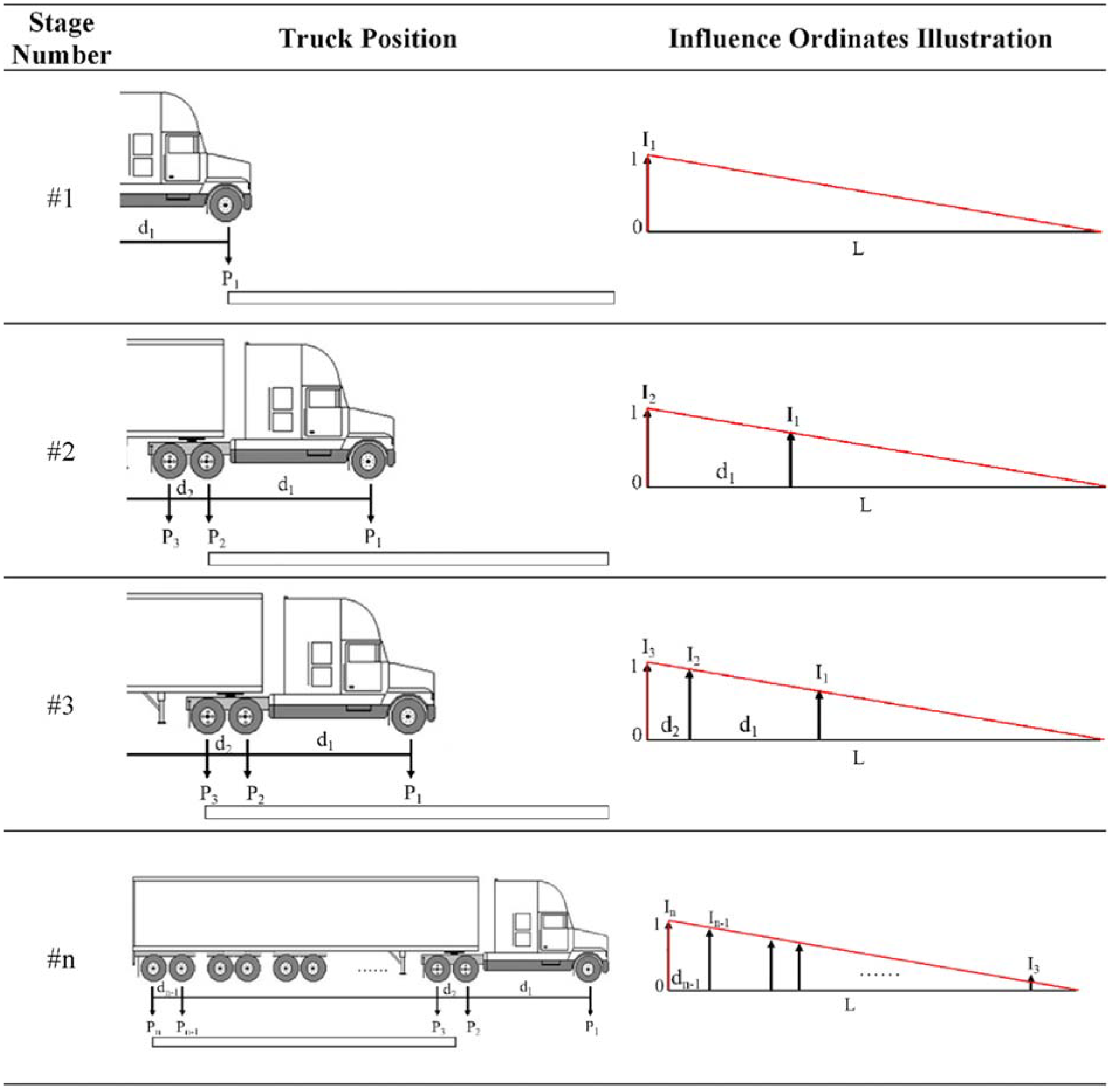
Truck position and influence ordinates.

Since the reaction force is equal to the summation of the product of axle weights and influence ordinates, n equations with n unknown axle weights can be constructed as follows.

Stage 1, Axle 1 arrives at the load cell: $P_{1} \cdot 1 + P_{2} \cdot 0 + P_{3} \cdot 0 + P_{4} \cdot 0 + P_{5} \cdot 0 = R_{1}$

Stage 2, Axle 2 arrives at the load cell: $P_{1} \cdot \frac{L - d_{1}}{L} + P_{2} \cdot 1 + P_{3} \cdot 0 + P_{4} \cdot 0 + P_{5} \cdot 0 = R_{2}$

Stage 3, Axle 3 arrives at the load cell: $P_{1} \cdot \frac{L - d_{2} - d_{1}}{L} + P_{2} \cdot \frac{L - d_{2}}{L} + P_{3} \cdot 1 + P_{4} \cdot 0 + P_{5} \cdot 0 = R_{3} \dots$

Stage n, Axle n arrives at the load cell: $P_{1} \cdot 0 + P_{2} \cdot 0 + \dots + P_{n - 1} \cdot \frac{L - d_{n - 1}}{L} + P_{n} \cdot 1 = R_{n}$

The axle weights can then be obtained by solving the n equations above. The GVW can be obtained by summing all the calculated axle weights. In general, for trucks with various numbers of axles, the influence ordinates can be constructed as an n-by-n matrix:

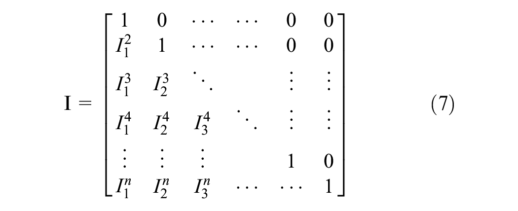
I = [\begin{matrix} 1 & 0 & \dots & \dots & 0 & 0 \\ I_{1}^{2} & 1 & \dots & \dots & 0 & 0 \\ I_{1}^{3} & I_{2}^{3} & ⋱ & ⋮ & ⋮ \\ I_{1}^{4} & I_{2}^{4} & I_{3}^{4} & ⋱ & ⋮ & ⋮ \\ ⋮ & ⋮ & ⋮ & 1 & 0 \\ I_{1}^{n} & I_{2}^{n} & I_{3}^{n} & \dots & \dots & 1 \end{matrix}]

(7)

where $I_{n}^{j}$ is the influence ordinate of the nth axle at the jth stage.

The axle weights (P) and reaction force (R) are both structured as n-by–1 matrices:

P = {[P_{1} P_{2} P_{3} \dots P_{n}]}^{T}

(8)

R = {[R_{1} R_{2} R_{3} \dots R_{n}]}^{T}

(9)

The final equation in matrix format is given by the following:

I \times P = R

(10)

The solutions of the axle weights are obtained by the following:

{P = R \times I}^{- 1}

(11)

The GVW is calculated as follows:

G V W = \sum_{1}^{n} P_{n}

(12)

Field Research Study

The proposed load cell-based B-WIM method was quantitively studied in the field using a slab-beam bridge located at Texas A&M University RELLIS Campus. Three trucks were used as test vehicles and traveled over the bridge at different speeds as well in different lanes. The recorded data was then processed to evaluate the accuracy of the methods. The following sections describe the bridge and the experimental tests.

Test Bridge Background

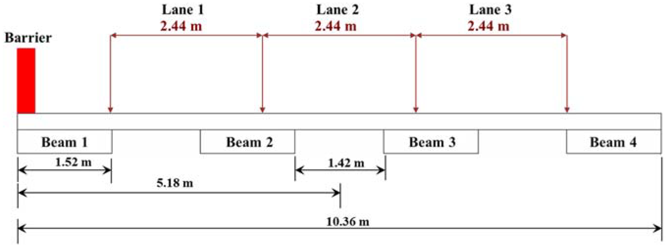
The test bridge is not in-service and is positioned at the edge of an old airport runway. This bridge was constructed for research purposes in 2015 ( 24 ) and is now utilized as a field laboratory. The structure is a prestressed concrete slab-beam bridge. The bridge has a 14.20 m (46.6 ft) span length (from center to center of the bearing pads) and an overall width of 10.36 m (34.0 ft). The bridge superstructure is comprised of four beams (TxDOT 5SB15) with prestressed concrete panel (PCP) stay-in-place forms. The 102 mm (4.0 in.) thick PCPs are 2.44 m (8.0 ft) long and have an overall width of 1.62 m (5.3 ft). To accommodate the camber of the prestressed slab beams, the cast-in-place (CIP) deck thickness varies slightly along the length. The minimum deck thickness (cast-in-place plus PCP) at the center of the bridge is 203 mm (8.0 in.). A typical section is shown in Figure 2.

Figure 2.

Bridge cross-section and vehicle paths (looking north).

A total of 16 load cells (two per bearing) were placed at both the north and south ends beneath each beam. The slab beams rest on top of elastomeric bearing pads (steel laminated). The load cell assemblies are between the bearing pads and the bridge abutment seat. Figure 3 shows a plan view of the bridge and the layout of the load cells. Note that the load cells were designed as part of the original bearing design for the bridge. Therefore, they were incorporated into the initial construction.

Figure 3.

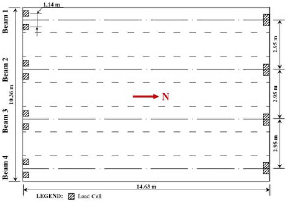
Bridge plan view and load cell layout.

Load Cells

There were two different load cell assemblies because of the different bearing configurations. At the south end of the bridge, there were two elastomeric bearing pads (229 mm × 229 mm) (9 in. × 9 in.) at the corners of the slab beams. At the north end of the bridge, the elastomeric bearing pads (229 mm × 457 mm) (9 in. × 18 in.) were at the center of the beam. The load cells were placed between a 25 mm (1.0 in.) thick bottom steel plate and a 38 mm (1.5 in.) thick top steel plate (see Figure 4).

Figure 4.

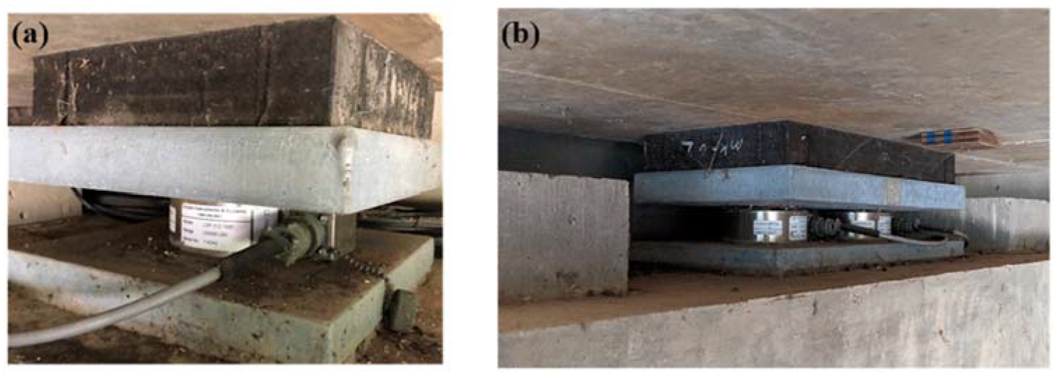
Bearing pads and load cells: (a) 229 mm × 229 mm bearing pad with one load cell and (b) 229 mm × 457 mm bearing pad with two load cells.

An array of commercially available load cells can be utilized for B-WIM. The load cells for this study (installed under a previous project) were Cooper LGP 312 100K compression-only pancake load cells with a 0–445 kN (100 kips) measurement range. These load cells provided a linearity of ±0.1% full scale and repeatability of ±0.03% full scale. The required load cell excitation was 10 Vdc with a bridge resistance of 350 ohms. The sampling rate of the load cells was set as 500 Hz. Figure 4a shows the 229 mm × 229 mm (9 in. × 9 in.) elastometric bearing pad with one load cell, while Figure 4b shows the 229 mm × 457 mm (9 in. × 18 in.) elastomeric bearing pad with two load cells.

Test Vehicles

Three vehicles with different weights and geometries were used for the B-WIM field study. For convenience, they are named Trucks A–C. The axle weights of the trucks were determined by calibrated static truck scales placed under each wheel. The resolution of the scales was 9 kg (20 lb). Then the GVWs were determined by summing the measured axle weights. Truck A is a tractor-trailer with five axles. The total weight of Truck A is 36,065 kg (79,510 lb). Trucks B and C are single-unit trucks (two axles) with static weights of 14,977 kg (33,020 lb) and 10,115 kg (22,300 lb), respectively. Figure 5, a–c, shows photos of each test truck and summarize the information of their axle weights and axle spacings. Note the axle spacing was obtained using a measuring tape. These dimensions were recorded to the nearest inch and then converted to the metric equivalent for reporting in this paper.

Figure 5.

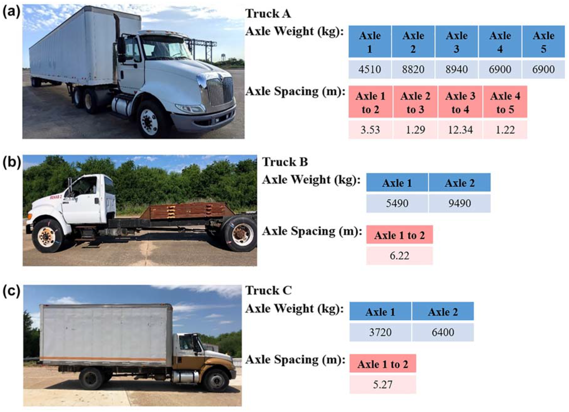
Test vehicles: (a) Truck A, gross vehicle weight (GVW) 36,070 kg, five axles, (b) Truck B, GVW 14,980 kg, two axles, and (c) Truck C, GVW 10,120 kg, two axles.

The bridge was divided into three (2.44 m [8 ft] wide) lanes to allow for more lateral vehicle configurations. These lanes are shown in Figure 2. For safety reasons, the first lane started 1.25 m (5 ft) away from the west edge of the bridge since the barrier impact capacity was minimal.

Full-Scale Tests

The load cells recorded a total of 50 single-vehicle tests (Truck A 15 tests, Truck B 14 tests, Truck C 21 tests) with speeds of approximately 16, 32, 48, 64, 80 km/h (10, 20, 30, 40, and 50 mi/h) on different lanes. Because of the safety concern, no trucks passed Lane 1 at 80 km/h (50 mi/h). Higher speeds were not possible because of the distance before and after the bridges. In addition, a total of four side-by-side tests were recorded with Trucks A and B traveling across Lanes 1 and 3 simultaneously.

Field Test Results

Axle Detection Results of Single-Truck Tests

The axle detection results were obtained by amplifying the change in load cell response through the second derivative of the signal. Figure 6 illustrates the measured data and the second derivative from the load cells underneath the south side of Beam 2, with Truck A passing the bridge from the south at 16 km/h (10 mi/h). In this particular test, the second derivative of the south side load cell data exhibits peaks when the truck enters the bridge. The negative peaks in the second derivative from the north side load cell data indicate the truck axles leaving the bridge. The number of axles can be obtained by counting the number of peaks, which can be automated using different peak picking algorithms.

Figure 6.

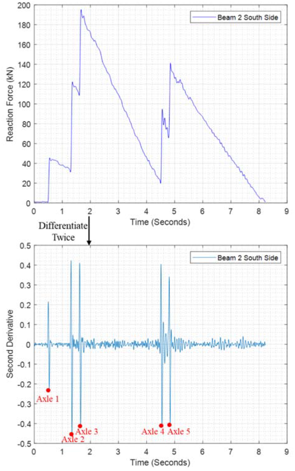
Measured load cell data and second derivative for Truck A in Lane 2 (16 km/h).

The truck average speed and axle spacing can be determined by implementing Equations 1 and 2, respectively. Figure 7 graphically demonstrates how the second derivative of the measured data (both ends shown) for a truck passage can be used to obtain the information needed to determine the truck average speed. Figure 8 illustrates how the second derivative information can be used for truck axle spacing.

Figure 7.

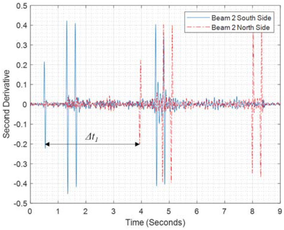
Second derivative data for Truck A in Lane 2 from the south at 16 km/h.

Figure 8.

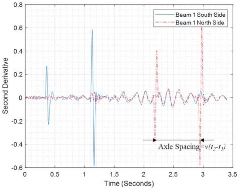
Second derivative data for Truck B in Lane 1 from the south at 32 km/h.

The accuracy of the results was evaluated using percent error. In this section, percent error was simply calculated as follows:

Error = \frac{C - M}{M} \times 100 %

(13)

where C is the calculated result and M is the measured (aka known) value from the radar gun, measuring tape, or static scales. Note that later in the paper, the results are summarized as percent accuracy since this is a standard WIM approach.

The average speed error of each truck test was analyzed and the histogram of the errors is shown in Figure 9a. The results have a mean value (µ) of 0.5% and a standard deviation (σ) of 4.5%. Figure 9b shows the empirical cumulative distribution function (CDF) of the errors with a lognormal fit. There are several factors that caused the relatively small errors. Firstly, the speed gun was held by an operator and there could be errors from the measuring angle as well as the speed gun itself. Secondly, the trucks were assumed to pass the bridge at a constant speed, but during the testing there could be minor acceleration or deceleration from the driver operations. Lastly, the noise in the measurements could be another cause of errors.

Figure 9.

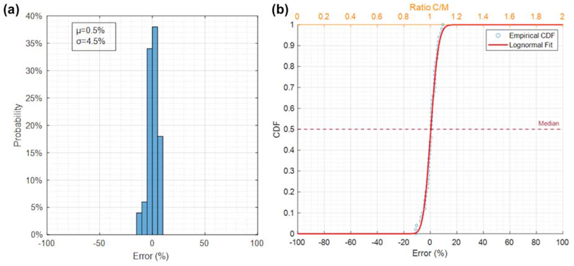
Average speed errors: (a) histogram and (b) cumulative distribution function (CDF).

The errors of axle spacing were calculated by comparing each obtained value with the axle spacing measured using a measuring tape. Figure 10 illustrates the histogram and CDF of errors of axle spacings, respectively. The mean of the errors is −0.9%, and the standard deviation is 5.1%. These results are considered acceptable because of the relatively low mean error and variability in the data. The primary source of the differences between the calculated and measured axle spacings were mainly from the average speed calculations (described above).

Figure 10.

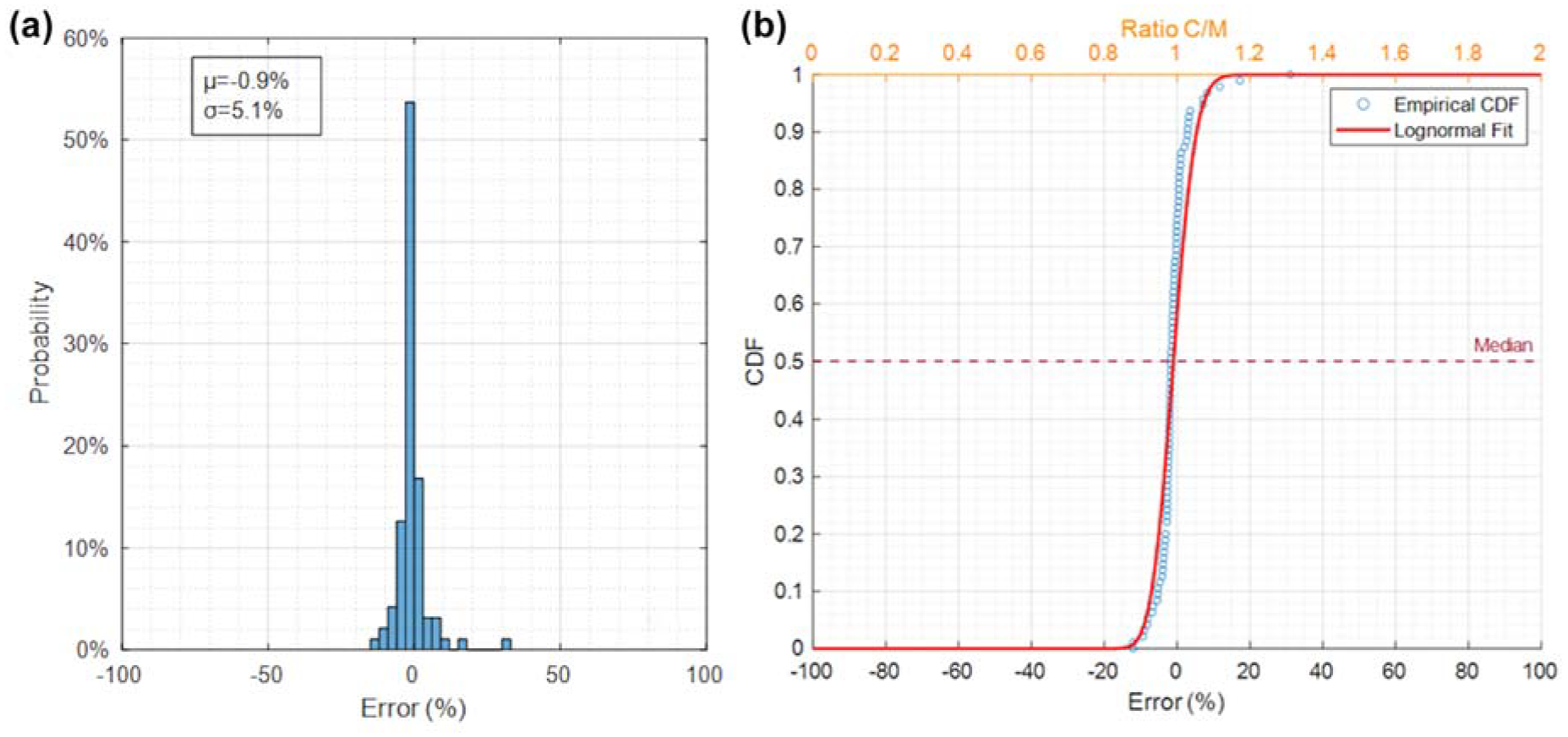
Axle spacing errors: (a) histogram and (b) cumulative distribution function (CDF).

The accuracy of the calculated axle spacings are important because these values are used in the reaction force method for weight calculations. Therefore, the higher accuracy of the axle spacing calculations reduces the cumulative error in the weight calculations.

Weight Calculation Results of Single-Truck Tests: Area Method

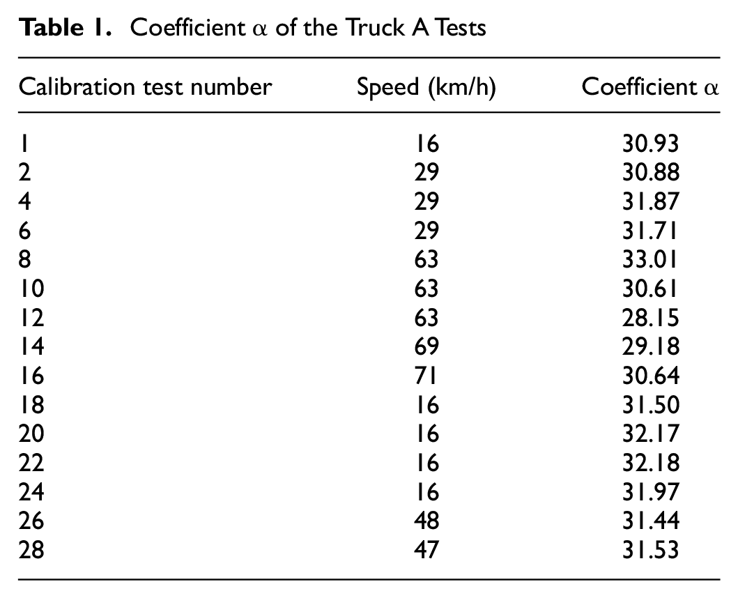
The GVW of each truck test was calculated based on calibration tests (Truck A tests) using the area method (explained earlier). The coefficient α was calculated by Equation 4. Table 1 shows the coefficient α values calculated from the 15 Truck A calibration tests, which illustrates the variability in results with respect to truck speed. The average value of α is 31.18. Equation 5 was then used to determine the GVWs of unknown vehicles (Trucks B and C). The mean value of the errors is −2.5%, with a standard deviation of 12.1%. Figure 11 shows the histogram and CDF of the GVW errors by the area method, respectively. These results are considered acceptable because of the relatively low mean error and variability but have room for improvement. The relative difference between the calculated GVWs and measured GVWs was caused by several factors. Firstly, only one truck was used as a calibration test truck and the α factor was taken as an average value. Secondly, the average speed calculation affects the area method. Thirdly, the static weight measurements were not repeated several times to minimize the measurement errors. Lastly, the varying dynamic effects induced by the passing trucks can influence the results.

Table 1.

Coefficient α of the Truck A Tests

Calibration test number	Speed (km/h)	Coefficient α
1	16	30.93
2	29	30.88
4	29	31.87
6	29	31.71
8	63	33.01
10	63	30.61
12	63	28.15
14	69	29.18
16	71	30.64
18	16	31.50
20	16	32.17
22	16	32.18
24	16	31.97
26	48	31.44
28	47	31.53

Figure 11.

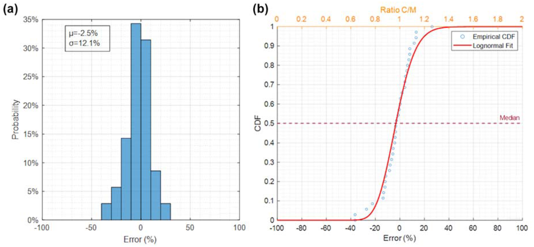
Gross vehicle weight errors: (a) histogram and (b) cumulative distribution function (CDF).

Weight Calculation Results of Single-Truck Tests: Reaction Force Method

The truck weight results were obtained from the reaction force method (explained earlier) and compared with the known weights (using static scales). The histogram and CDF of errors for GVWs is shown in Figure 12. The calculated GVW errors have a mean of −9.0% and a standard deviation of 7.0%. The calculated axle weights of each truck have errors with a mean of −8.2% and a standard deviation of 13.7%, as shown in Figure 13. The larger spread of results for axle weights compared to GVWs is consistent with prior studies, as stated earlier. It can be observed that the GVW and axle weight mean values are biased (or shifted). This was investigated, and the reason is because of using the second derivative method for identifying the specific time each axle crosses the load cells. As a result, there was a slight shift between the corresponding peak locations of the datasets. The exact time of the second derivative calculation does not precisely coincide with the point in time the axles are over the center of the load cells. This can be corrected (or calibrated) through offset of the data but was not presented here to show the true results. Note that this shift is consistent, so the calculations of the number of axles, axle spacing, and average speed are not affected since they are directly obtained from the second derivative data.

Figure 12.

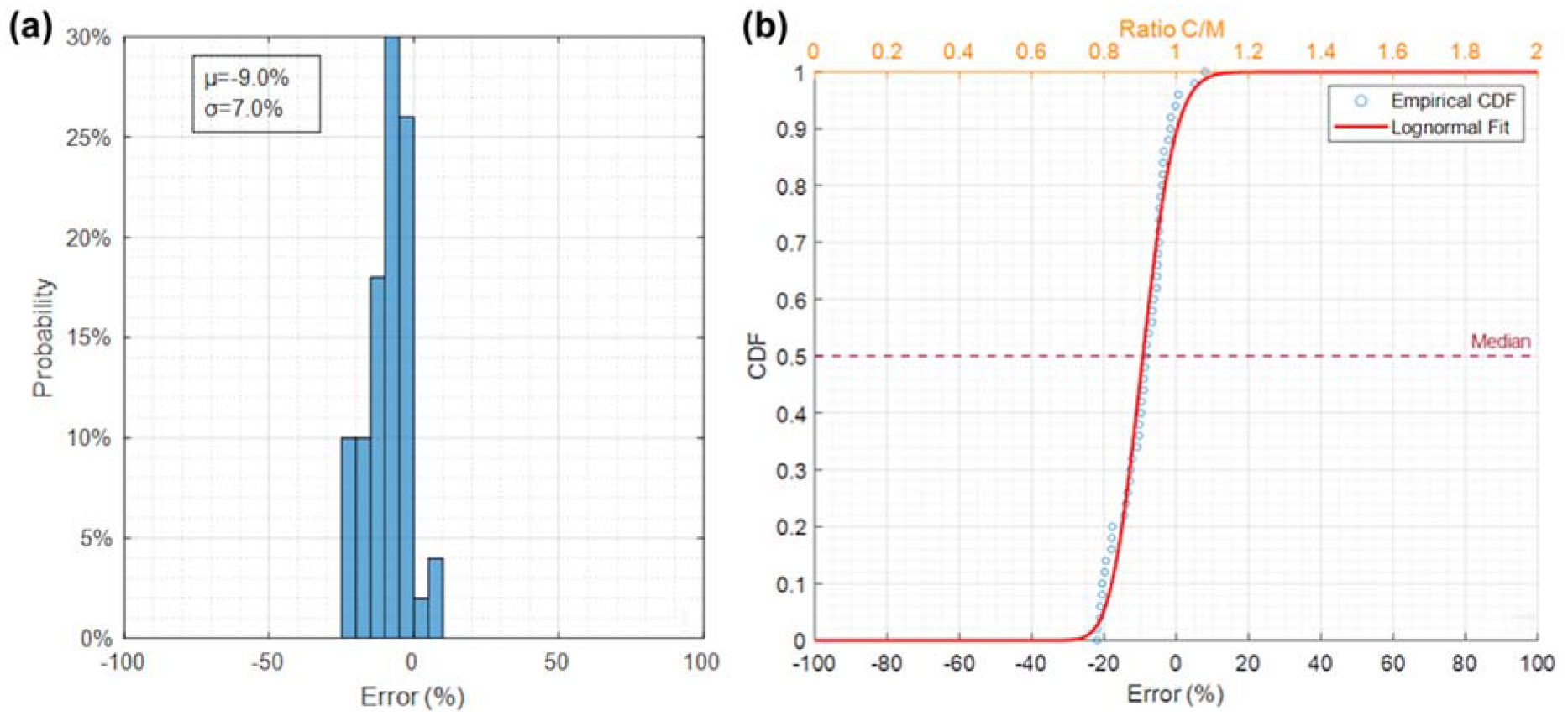
Gross vehicle weight errors by the reaction force method: (a) histogram and (b) cumulative distribution function (CDF).

Figure 13.

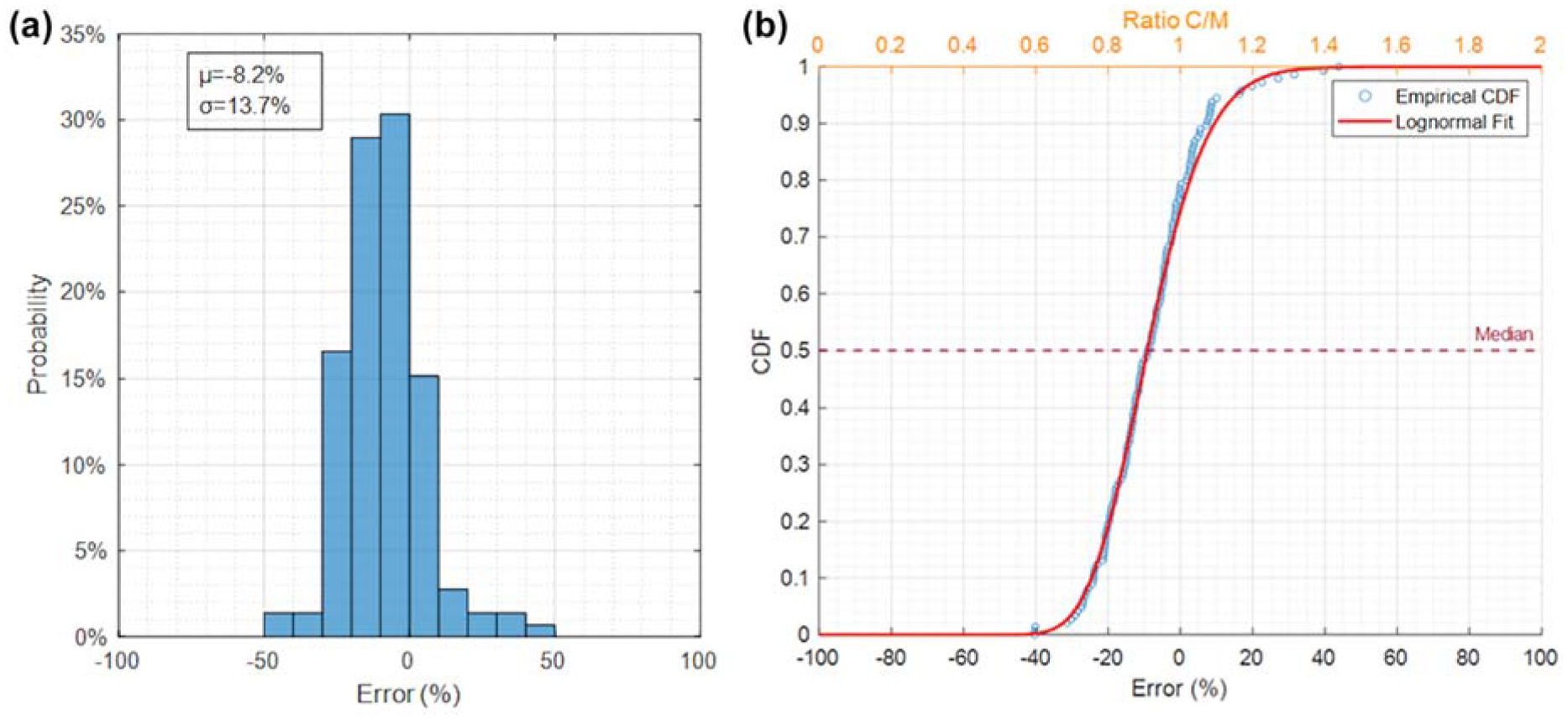
Axle weight errors by the reaction force method: (a) histogram and (b) cumulative distribution function (CDF).

Summary of the Single-Truck Test Results

To evaluate the performance of the proposed load cell-based B-WIM algorithms, the errors were converted to accuracies as follows:

Accuracy = \frac{\sum_{1}^{m} (1 - | Error |)}{m} \times 100 %

(14)

where m is the number of data points. The accuracy here represents the average accuracy of the calculated truck axle information or weight results.

Table 2 summarizes the average accuracy of the axle and weight information from the preliminary algorithms and sensors. Overall, the axle detection results were excellent, with at least 97% accuracy in all categories. The weight calculations were very good for GVW with 91% accuracy and axle weight with 87% accuracy (using Equation 14). For the B-WIM system, the axle weights are consistently the most difficult to identify. Only a 4% reduction in accuracy from GVW to axle weight is a significant improvement from that observed in the literature.

Table 2.

Average Accuracy of Axle and Weight Information Determination

Parameters	Axle information average accuracy
Number of axles	100%
Average speed	97%
Axle spacing	97%
	Weight information average accuracy
	Area method	Reaction force method
GVW	91%	91%
Axle weight	na	87%

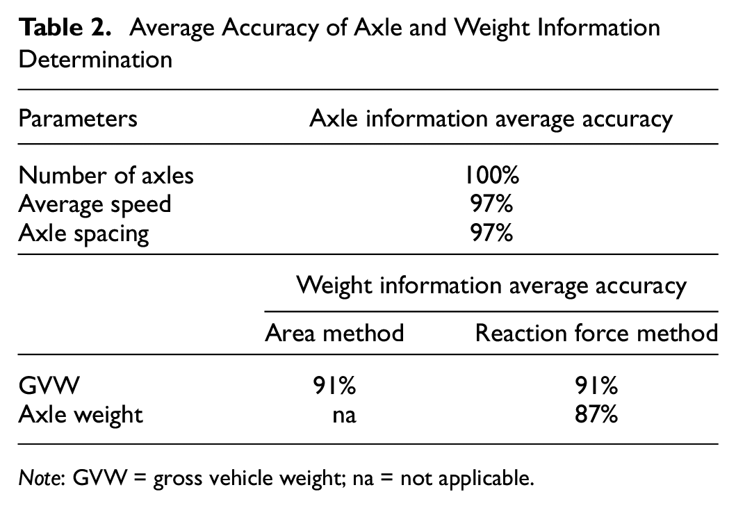
Note: GVW = gross vehicle weight; na = not applicable.

The research team recognizes that the accuracies shown are relatively high. These accuracies may be reduced for in-service bridges because of the limitations of the presented study. Firstly, only three test trucks were utilized because of resource limitations. In-service bridges will experience a wide array of vehicles passing the bridge. Another limitation of the research is the presence of side-by-side trucks. This is addressed in the following section.

Side-by-Side Cases: Discussion

The individual GVW of the side-by-side trucks can be relatively challenging for B-WIM systems. In this study these side-by-side GVWs were obtained by utilizing the area method and midspan distribution factors. For example, consider that Truck A travels on Lane 1 (left-hand lane), while Truck B travels on Lane 3 (right-hand lane). The combined GVW (GVW_total) of the two trucks can be obtained by the area method introduced previously (assume two trucks pass the bridge with the same speed). The load cell distribution factor for this truck passing event (DF_i) can be determined by the following:

{D F}_{i} = \frac{r_{i}}{\sum_{1}^{N} r_{i}}

(15)

where N is the number of beams and r_i is the reaction force of the ith beam. By calculating the DF of each test, the average distribution factors when one truck passes the left-hand lane (DFL_i) and the right-hand lane (DFR_i) can be obtained. Using the ith beam, two equations can be constructed as follows:

{G V W}_{A} + {G V W}_{B} = {G V W}_{t o t a l}

(16)

{D F L}_{i} \cdot {G V W}_{A} + {D F R}_{i} \cdot {G V W}_{B} = {D F}_{i} \cdot {G V W}_{t o t a l}

(17)

The gross weight of each truck (GVW_A and GVW_B) can be determined by solving the equations.

The distribution factors of each single-truck test were calculated and the results were averaged to get the DFL and DFR values. The DFL, DFR, and DF values of the four side-by-side tests (named S1–S4) are summarized in Table 3. It should be noted that in Tests S1–S3, Truck A (36,065 kg static weight) traveled on Lane 1 and Truck B (14,977 kg static weight) traveled on Lane 3. In Test S4, Truck A traveled on Lane 3 and Truck B traveled on Lane 1.

Table 3.

Load Cell Distribution Factor Summary

Configuration	Distribution factor
Configuration	Beam 1	Beam 2	Beam 3	Beam 4
DFL	0.35	0.56	0.08	0.01
DFR	0.01	0.05	0.57	0.37
DF
Test S1	0.29	0.36	0.23	0.12
Test S2	0.28	0.37	0.22	0.13
Test S3	0.27	0.35	0.21	0.16
Test S4	0.15	0.22	0.36	0.27

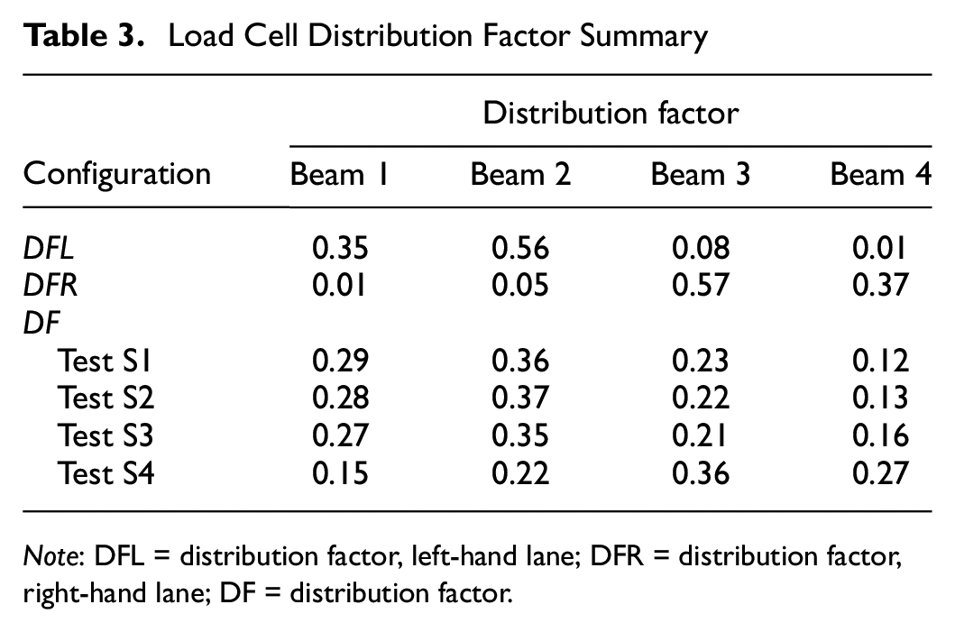
Note: DFL = distribution factor, left-hand lane; DFR = distribution factor, right-hand lane; DF = distribution factor.

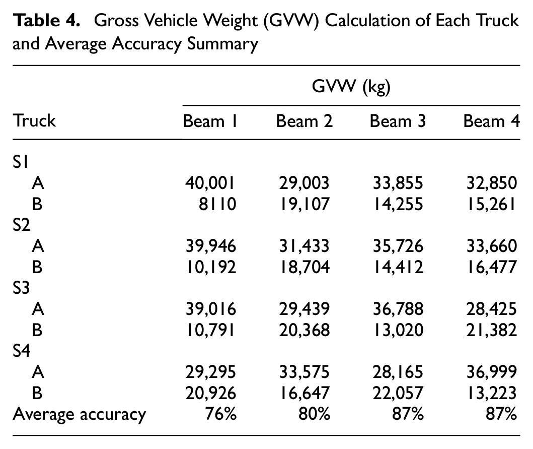
The weight of each truck of the side-by-side tests was calculated using the results for each beam. As summarized in Table 4, it was found that when using the distribution factor for calculating the weight of side-by-side trucks, the average accuracy ranged from 76% to 87%. Since the individual weight of each truck is distributed from the sum weight of the trucks using this method, the accuracy is significantly influenced by the accuracy of GVW_total calculation by area method.

Table 4.

Gross Vehicle Weight (GVW) Calculation of Each Truck and Average Accuracy Summary

Truck	GVW (kg)
Truck	Beam 1	Beam 2	Beam 3	Beam 4
S1
A	40,001	29,003	33,855	32,850
B	8110	19,107	14,255	15,261
S2
A	39,946	31,433	35,726	33,660
B	10,192	18,704	14,412	16,477
S3
A	39,016	29,439	36,788	28,425
B	10,791	20,368	13,020	21,382
S4
A	29,295	33,575	28,165	36,999
B	20,926	16,647	22,057	13,223
Average accuracy	76%	80%	87%	87%

Future Research

The research team has identified several areas of focus for future work. The research presented above was the findings from the first phase of a larger B-WIM study. Some of the primary future research areas include the following.

1) Exploration of improved data processing techniques: In the data processing, the central differences were used for obtaining the second derivatives. This method may not be the most accurate way to differentiate the data. Other methods, such as considering adaptive step size or a higher-order numerical differentiation scheme, will be explored.

2) Improvement of axle detection accuracy: In the peak detection process, there could be cases where noise in the measurement produces sharp changes as the peaks are similar to the passing axles. This can be improved through enhanced filtering methods or by adding the physical meaning to the data processing algorithm. For example, adding the minimum and maximum axle spacing limitation when picking peaks.

3) Improvement of axle weight calculation accuracy: The axle weight accuracies can be improved through enhanced data processing and axle detection methods (discussed in the prior two points). In addition, refinement of the methodology to consider nonlinear behavior could further improve the axle weight calculations.

4) Investigation of the multi-vehicle scenarios: The initial research focused on single-truck events within any lane and only a few side-by-side tests were conducted. Beam distribution factors were utilized to get the individual truck weights in a side-by-side event. More tests need to be conducted to further adjust the algorithms and improve the accuracy. Three-dimensional finite element method (3D FEM) can also be developed for a similar purpose.

Conclusions and Recommendations

This paper quantitatively evaluates B-WIM systems using load cells as an alternative to conventional strain-based B-WIM systems. Full-scale field tests were conducted to assess the performance. The second derivative approach was utilized for processing axle detection, and the area method and reaction force method were studied for GVW and axle weight calculation. Side-by-side cases were explored utilizing the beam distribution factors. The following general conclusions were drawn from the load cell-based B-WIM study.

1) The number and spacings of axles, along with vehicle speed, can be accurately obtained using the second derivative of the load cell data. The experimental test results produced average accuracies ranging from 97% to 100% in these areas.

2) The axle weights can be identified from load cell data using the reaction force method with a reasonable accuracy (average accuracy of 87%). The GVW can then be obtained by summing the axle weights (average accuracy of 91%). These results are without any calibration tests. Calibration can be performed to improve the accuracy.

3) The GVW may be accurately determined using the area method with load cell data. The results of this study indicate slightly better accuracy than the reaction force method (average accuracy of 91%). However, the area method can only obtain GVWs (not axle weights), and calibration tests are required.

4) The total weight of the two trucks in a side-by-side event can be determined using the area method. The approach to calculate individual truck weights was to utilize the beam distribution factors identified in the calibration tests, which produced reasonable GVW results (average accuracies ranging from 76% to 87%). However, to achieve this accuracy, the bridge span length should be relatively short to avoid back-to-back trucks on the structure at the same time.

The research team has shown the potential for the use of load cells in B-WIM systems by quantitively evaluating the performance on a full-scale structure. However, future research and long-term validation is recommended before application on in-service bridges. Logistically the use of load cells can be challenging for existing bridges. The best situation is to have load cells installed during the construction of a new bridge or during bearing replacement. With respect to algorithms, the processing of axle information using the second derivative of the data showed promising results in this study. The reaction force method is recommended for weight identification since it can determine axle and gross truck weights without calibration of the system. However, if calibration is possible, then including the area method can improve the robustness of the B-WIM system.

Footnotes

Acknowledgements

The authors want to thank the TxDOT program manager, Martin Dassi, along with the TxDOT research panel members, Bernie Carrasco, Biniam Aregawi, David Fish, David Freidenfeld, Drake Builta, and Mark Wallace. In addition, the authors would like to thank Mary Beth Hueste and Tevfik Terzioglu from Texas A&M University for their support with the RELLIS Bridge.

Author Contributions

The authors confirm contribution to the paper as follows: study conception and design: S. Shi, M. Yarnold, J. Mander; data collection: S. Shi, M. Yarnold, S. Hurlebaus; analysis and interpretation of results: S. Shi, M. Yarnold, J. Mander; draft manuscript preparation: S. Shi, M. Yarnold. All authors reviewed the results and approved the final version of the manuscript.

Declaration of Conflicting Interests

The author(s) declared no potential conflicts of interest with respect to the research, authorship, and/or publication of this article.

Funding

The author(s) disclosed receipt of the following financial support for the research, authorship, and/or publication of this article: This material is based on work supported by the Texas Department of Transportation (TxDOT) through Project 0-7038—“Develop Bridge Weigh-in-Motion Approach to Measure Live Loads on Texas Highways.”

ORCID iDs

Shengyi Shi

Matthew Yarnold

Stefan Hurlebaus

Any opinions, findings, and conclusions, or recommendations expressed in this material are those of the authors and do not necessarily reflect the views of the Texas Department of Transportation.

References

Moses

Weigh-in-Motion System Using Instrumented Bridges. Journal of Transportation Engineering, Vol. 105, 1979, pp. 233–249. https://doi.org/10.1061/TPEJAN.0000783.

Žnidaric

Lavric

Kalin

Free-of-Axle Detector Bridge WIM Measurements on Short Slab Bridges. Proc., 3rd International WIM Conference, Orlando, FL,Iowa State University located at Ames, IA, 2002, pp. 231–239.

Kalin

Žnidarič

Lavrič

Practical Implementation of Nothing-on-the-Road Bridge Weigh-in-Motion System. Proc., International Symposium on Heavy Vehicle Weights and Dimensions, State College, PA, 2006.

Kumar

Schultz

Hourdos

Enriched Sensor Data for Enhanced Bridge Weigh-in-Motion (eBWIM) Applications. Center for Transportation Studies, University of Minnesota, 2018.

O’Brien

Hajializadeh

Uddin

Robinson

Opitz

Strategies for Axle Detection in Bridge Weigh-in-Motion Systems. Proc., International Conference on Weigh-in-Motion (ICWIM 6), Dallas, TX, John Wiley & Sons, Hoboken, NJ, 2012, pp. 79–88.

Helmi

Taylor

Ansari

Shear Force–Based Method and Application for Real-Time Monitoring of Moving Vehicle Weights on Bridges. Journal of Intelligent Material Systems and Structures, Vol. 26, 2015, pp. 505–516. https://doi.org/10.1177/1045389X14529612.

Bao

Babanajad

S. K.

Taylor

Ansari

Generalized Method and Monitoring Technique for Shear-Strain-Based Bridge Weigh-in-Motion. Journal of Bridge Engineering, Vol. 21, 2016, p. 04015029. https://doi.org/10.1061/(ASCE)BE.1943-5592.0000782.

Kalhori

Alamdari

M. M.

Zhu

Samali

Mustapha

Non-intrusive Schemes for Speed and Axle Identification in Bridge-Weigh-in-Motion Systems. Measurement Science and Technology, Vol. 28, 2017, p. 025102. https://doi.org/10.1088/1361-6501/aa52ec.

Aguilar

S. L.

Christenson

R. E.

A Simplified Shear-Strain Based Bridge Weigh-in-Motion Method for In-Service Highway Bridges. Métodos y Materiales, Vol. 8, 2018, pp. 11–22. https://doi.org/10.15517/mym.v8i1.34551.

10.

Sekiya

Kubota

Miki

Simplified Portable Bridge Weigh-in-Motion System Using Accelerometers. Journal of Bridge Engineering, Vol. 23, 2018, p. 04017124. https://doi.org/10.1061/(ASCE)BE.1943-5592.0001174.

11.

Choo

J. F.

D.-H.

Chang

S.-G.

Lee

D.-H.

Cho

C.-B.

New Bridge Weigh-in-Motion System Using Piezo-Bearing. Shock and Vibration, Vol. 2018, 2018, p. 6185695. https://doi.org/10.1155/2018/6185695.

12.

Ojio

Carey

OBrien

E. J.

Doherty

Taylor

S. E.

Contactless Bridge Weigh-in-Motion. Journal of Bridge Engineering, Vol. 21, 2016, p. 04016032. https://doi.org/10.1061/(ASCE)BE.1943-5592.0000776.

13.

O’Brien

E. J.

Rowley

Gonzalez

A Regularised Solution to the Bridge Weigh in Motion Equations. International Journal of Heavy Vehicle Systems, Vol. 16, 2009, pp. 310–327.

14.

Lydon

Taylor

S. E.

Doherty

Robinson

O’Brien

E. J.

Žnidarič

Bridge Weigh-in-Motion Using Fibre Optic Sensors. Proceedings of the Institution of Civil Engineers-Bridge Engineering, Vol. 170, No. 3, 2017, pp. 219–231.

15.

Dubbs

N. C.

Design of Instrumented Bearings for Direct Measure of Bridge Live Loads. Proc., IABSE Symposium: Engineering the Future, Vancouver, Canada, IABSE, Zurich, Switzerland, September 21–23, 2017, pp. 1553–1560.

16.

Cho

J.-R.

Kim

Y. J.

Kwark

J.-W.

Park

S. Y.

Chin

W. J.

Kim

B.-S.

Load-Measuring Pot Bearing with Built-In Load Cell—Part I: Design and Performance. Engineering, Vol. 5, 2013, p. 856.

17.

Ojio

Yamada

Bridge Weigh-in-Motion Systems Using Stringers of Plate Girder Bridges. Proc., Third International Conference on Weigh-in-Motion (ICWIM3), Iowa State University, Ames, 2002.

18.

Ojio

Yamada

Bridge WIM by Reaction Force Method. Proc., 4th International Conference on Weigh-In-Motion, Taipei, Taiwan, 2005.

19.

Wang

Zhu

Mao

Zhao

Identification of Moving Train Loads on Railway Bridge Based on Strain Monitoring. Smart Structures and Systems, Vol. 23, 2019, pp. 263–278. https://doi.org/10.12989/sss.2019.23.3.263.

20.

Zhao

Cloud-Based Real-Time Continuous Bridge Monitoring: Bridge Weigh in Motion and Condition Assessment. Doctoral dissertation. Tufts University, Medford, MA, 2017.

21.

Christenson

Bakulski

McDonnell

A.-M. H.

Establishment of a Dual-Purpose Bridge Health Monitoring and Weigh-in-Motion System for a Steel Girder Bridge. Presented at 90th Annual Meeting of the Transportation Research Board, Washington, D.C., 2011, p. 16.

22.

Helmi

Bakht

Mufti

Accurate Measurements of Gross Vehicle Weight Through Bridge Weigh-in-Motion: A Case Study. Journal of Civil Structural Health Monitoring, Vol. 4, 2014, pp. 195–208. https://doi.org/10.1007/s13349-014-0076-5.

23.

Algohi

Mufti

Bakht

BWIM with Constant and Variable Velocity: Theoretical Derivation. Journal of Civil Structural Health Monitoring, Vol. 10, 2020, pp. 153–164. https://doi.org/10.1007/s13349-019-00377-0.

24.

Hueste

M. B. D.

Mander

J. B.

Terzioglu

Jiang

Petersen-Gauthier

Spread Prestressed Concrete Slab Beam Bridges. Texas A&M Transportation Institute, College Station, 2015.

Evaluation of a Load Cell-Based Bridge Weigh-in-Motion System

Abstract

Keywords

Research Objectives

Methodology

Vehicle Axle Detection

Vehicle Weight Calculation

Area Method

Reaction Force Method

Field Research Study

Test Bridge Background

Load Cells

Test Vehicles

Full-Scale Tests

Field Test Results

Axle Detection Results of Single-Truck Tests

Weight Calculation Results of Single-Truck Tests: Area Method

Weight Calculation Results of Single-Truck Tests: Reaction Force Method

Summary of the Single-Truck Test Results

Side-by-Side Cases: Discussion

Future Research

Conclusions and Recommendations

Footnotes

Acknowledgements

Author Contributions

Declaration of Conflicting Interests

Funding

ORCID iDs

References