
Abstract
Reliable geotechnical site characterization and geohazard assessment are critical for bridge foundation design and management. This paper explores existing and emerging artificial intelligence-machine learning methods (AI-ML) transforming geotechnical site characterization and scour assessment for bridge foundation design and maintenance. The prevalent ML techniques applied for subsurface characterization are reviewed, and step-by-step methodologies for stratigraphy classification, borehole interpretation, geomaterial characterization, and ground modeling are provided. The ML techniques for maximum scour depth prediction are reviewed, and a simple ML methodology is proposed to provide a more reliable tool for scour depth estimation for implementation in practice. Also, a novel deep learning approach, with a detailed implementation description, is recommended for real-time scour monitoring and assessment of existing bridges. The challenges with database design and data processing for ML modeling, model optimization, training and validation, and uncertainty assessments are discussed, and innovative techniques for addressing them are reviewed.
Keywords
Reliable geotechnical site characterization and geohazard assessment are critical elements in bridge infrastructure design and management. Scour, a major geohazard affecting bridges over waterways, is the main cause of failure in the United States and worldwide ( 1 – 3 ). In this paper, we review emerging artificial intelligence (AI) and machine learning (ML) technologies that are transforming geotechnical site characterization and scour assessments for bridge foundation design and maintenance.
AI, a versatile field encompassing ML, data analytics, and computational modeling, has catalyzed transformative change across various industries. Geotechnical engineering is no exception, benefiting from AI’s capabilities to extract valuable insights, enhance predictive accuracy, and optimize decision-making processes, considering geohazards. This fusion of geotechnical engineering and AI has far-reaching implications, promising safer and more reliable infrastructure, cost savings, and minimized environmental impact.
There are state of the art reviews on ML/deep learning (DL) applications in geotechnical engineering, including Yousefpour and Fallah’s ( 4 ) on ML applications in geotechnics, Zhang et al.’s ( 5 ) on DL applications in geotechnical engineering and ML modeling of soil properties ( 6 ), Dikshit et al.’s ( 7 ) on geohazard modeling, Tehrani et al.’s ( 8 ) landslide studies and recently Phoon and Zhang’s ( 9 ) review on the future of ML in geotechnics.
The objective of this discussion is to highlight the recent advances and underscore the importance of continued research and innovation in harnessing the full potential of AI-ML for safer, more resilient, and cost-effective bridge foundations. The paper is organized as follows. The next section introduces the synopsis on AI and ML. We then present subsurface characterization and scour assessment using ML. We also provide recommendations with step-by-step implementation methods for applications in practice. We end the paper with a conclusion section.
Synopsis on Artificial Intelligence and Machine Learning
AI and ML represent two dynamic and interrelated fields at the forefront of modern technology. AI is a broader concept, encompassing the development of intelligent systems capable of tasks traditionally requiring human intelligence, such as problem solving, language understanding, and decision making. ML, on the other hand, is a subset of AI focused on the development of algorithms that enable computers to learn from and make predictions or decisions based on data.
AI and ML have seen unprecedented growth and application across various industries. In the domain of AI, natural language processing (NLP) has enabled conversational AI and language translation ( 10 ). Computer vision has transformed image and video analysis ( 11 ), while reinforcement learning has empowered robots and autonomous systems ( 12 ). Meanwhile, ML techniques, including supervised learning, unsupervised learning, and reinforcement learning, have revolutionized data-driven decision-making processes in fields ranging from health care and finance to engineering applications ( 13 , 14 ). The synergy between AI and ML is evident in their iterative and data-centric approach. ML algorithms learn patterns from data and improve their performance over time, aligning with the AI goal of creating intelligent, adaptive systems. Additionally, the availability of vast data sets and increased computing power has fueled the advancement of AI and ML applications.
Deep learning employs artificial neural networks inspired by the human brain to solve complex problems ( 15 ). DL has revolutionized AI by enabling breakthroughs in computer vision, natural language processing, and speech recognition ( 16 ). Convolutional neural networks (CNNs) ( 17 ) have enhanced image recognition, while recurrent neural networks (RNNs) ( 18 ) and transformer models ( 19 ) have elevated language understanding and generation to unprecedented levels. Generative AI is the most recent advancement in this field, creating systems capable of generating content, such as images, text, music, and more, often with remarkable creativity. At its core, generative AI seeks to enable machines to produce novel, human-like output. The driving force behind many generative AI models is the use of neural networks, particularly generative adversarial networks (GANs) ( 20 ).
In civil engineering, AI-ML has been used mostly in structural health and performance monitoring ( 21 – 23 ), design optimization ( 24 ), predictive maintenance ( 25 ), construction automation and management ( 11 , 26 ), transport planning ( 27 ), and in various aspects of geotechnical engineering ( 4 , 5 ).
Subsurface Characterization Using ML
Subsurface characterization, including stratigraphic configuration and the associated geotechnical properties, has long been a challenge in geotechnical practice. Because of the geological processes leading to the compounded deposition and subsequent changes of geomaterials, including layering, each stratum exhibits variation from point to point within a volume ( 28 ). Nevertheless, the identification of subsurface stratification and the characterization of spatially varying soil and rock properties with the limited availability of site investigation information are indispensable for site characterization and following design analyses.
The TC309 (International Society for Soil Mechanics and Geotechnical Engineering [ISSMGE]’s Technical Committee for Machine Learning and Big Data) carried out an online survey in 2019, receiving 114 responses. The survey highlighted that machine learning is expected to have a significant impact on geotechnical site characterization among others. Site characterization is one of the leading areas where machine learning can transform practice over the next 10 years (Figure 1).
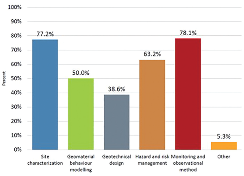
Machine learning survey: What are the machine learning applications that can transform value for our industry in the next 10 years? (Select all that apply).
Stratigraphy Classification
Stratigraphy classification is essential in site investigation, as it provides the necessary knowledge on the geological body ( 29 ). For example, the significance of the stratigraphy classification might be observed in the failure of a slope consisting of multiple strata, in which the failure is often dominated by the spatial distribution of the weak stratum ( 30 ). However, the subsurface stratigraphic configuration at a site is hard to characterize accurately because of the complexity and inherent spatial variability of the strata and the limited availability of exploration data.
The essence of stratigraphic modeling is a process of interpolating and predicting strata of the whole area of interest from a limited amount of known data ( 31 ). It generally treats geological units as discrete variables, such as stratigraphic classes or rock classes, and thus formulates the modeling task as a classification problem corresponding to discrete variables. DL and ML are the methods that learn a model with statistical characteristics from known data and use the model to make judgments and predictions about new scenarios. In this way, the principles of stratigraphic modeling fit with DL and ML ( 32 ).
In recent years, there has been a boom in research on the stratigraphy classification based on DL or ML. As listed in Table 1 ( 33 ), the possibility of various machine learning algorithms in handling stratigraphy classification tasks has been verified, from shallow classification algorithms, such as convolutional neural networks (CNN), eXtreme gradient boosting (XGBoost), support vector machines (SVM), decision tree (DT), random forest (RF), and maximum likelihood, to variants of neural networks, such deep feed-forward neural networks (DFNN), RNNs, graph neural networks (GNN), and GAN. The modeling ideas of these methods may be divided into stratigraphy classification methods based on the image analysis and those based on the borehole interpretation.
Summary of DL and ML Algorithms Used in Stratigraphy Classification
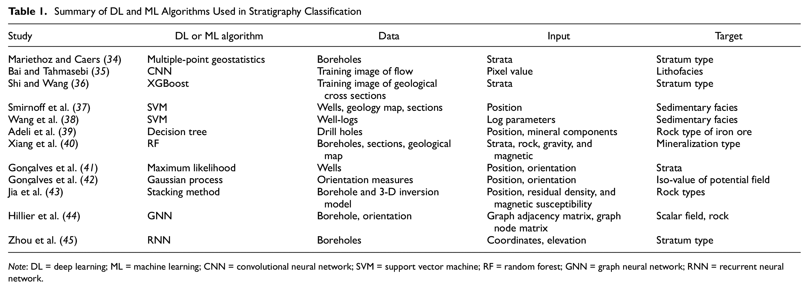
Note: DL = deep learning; ML = machine learning; CNN = convolutional neural network; SVM = support vector machine; RF = random forest; GNN = graph neural network; RNN = recurrent neural network.
The above studies have established the foundation for the application of machine learning to stratigraphy classification. In addition, they also reveal the characteristics of different approaches. Traditional machine learning classifiers are suitable for learning tasks with small samples, while DL algorithms dominated by neural networks generally require large amounts of training data to obtain better learning results. However, it is always troublesome to acquire and label geological data. The samples are too sparse to represent the feature space effectively, thus limiting to some extent the performance of DL models in geological reconstruction tasks.
Image Analysis
The depositional stratigraphic relationships can be quantitatively reflected in a training image (TI), which can be defined as a conceptual representation of the expected subsurface heterogeneities in the area of interest. Stochastic conditional simulation methods using TIs, for example, multiple-point statistics ( 34 – 46 ) and iterative convolution XGBoost ( 47 ), have been developed to depict stratigraphic connectivity between soil deposits. These image-based stochastic simulation algorithms have been successfully applied to tackle practical geotechnical problems, for example, reclamation and slope stability ( 48 ).
A TI is an ensemble of prior geological knowledge, which enables quantitative incorporation of subjective geological interpretation of a studied domain, and it can be directly obtained from a nearby site or previous projects with similar geological settings. The idea of TI is appealing to geological and geotechnical practitioners as it can effectively leverage on prior geological knowledge in a quantitative manner and combat the problem of scarce geological data often encountered in the development of subsurface geological cross sections. It should be noted that the performance of stochastic simulation methods for subsurface geological modeling can be greatly influenced by TI particularly when site-specific measurements are limited, and an improper TI may lead to geological realizations incompatible with observed data or even false interpretation of geological processes ( 49 , 50 ). This underscores the importance of selecting a proper TI for stochastic simulation methods.
Image-based stochastic simulations learn stratigraphic features from a single training image and leverage on the extracted patterns to yield an alternative representation of subsurface stratigraphy while conditioning on available site-specific data (e.g., slope outcrops or borehole logs). A training image can be viewed as a prior ensemble of local geological knowledge and experience (e.g., inter-relationships between soil types and orientations of soil layer boundaries) with the required spatial scale at the site of interest. More specifically, a qualified training image is a numerical representation of believed stratigraphic heterogeneities. Although it does not necessarily enclose all the detailed stratigraphic features at a target site, it should exhaust major repetitive stratigraphic relationships and structures ( 34 ). Training images essentially serve as effective supplements to overcome challenges associated with data sparsity, which is an intrinsic issue in geotechnical site investigation and geological modeling.
Shi and Wang ( 36 ) proposed a framework for the conditional simulation of subsurface stratigraphy, based on the typical cross sections for weathered granite and tuff slopes in Hong Kong. Subsequently, the proposed framework was applied to delineate subsurface stratigraphy and quantify associated stratigraphic uncertainty using real slope cross sections in Hong Kong. In the context of this framework, the inputs are the images of the geological cross sections. The geological cross section predicted by this framework is dependent on both the training image adopted (i.e., a prior geological model) and site-specific measurements (i.e., likelihood information). There is a balance between the prior geological model and site-specific measurements. Prior geological knowledge governs the posterior subsurface system when available measurements are limited. However, the influence of a training image weakens as the number of site-specific measurements increases (or likelihood information strengthens), and the final predicted geological cross section will be mainly dominated by site-specific data when many measurements are taken from a specific site. The basic structure of this proposed framework can be summarized with the following steps.
Step 1. Collecting Training Images
The first step for establishing a training image database is to collect many geological cross sections from different sources and digitalize them using a consistent format. The potential training images can be obtained from four different sources: 1) the delineation of subsurface geological cross sections is a must for every geotechnical project, and it is, therefore, natural to collect geological cross sections developed from previous projects and use them as training images; 2) conceptual geological models developed by engineering practitioners, or even hand drawn by experienced geologists, can also be used as training images; 3) a training image can also be simulated using different generative models such as object-based, process-based, and process-mimicking models, for example, Mariethoz and Caers ( 34 ); and 4) training images can snapshots taken directly from experiments using small-scale models.
Step 2. Categorizing Training Images
To facilitate the subsequent selection of training images for subsurface stratigraphy, all the collected training images may be further classified into different categories in accordance with their geological origin, location, and application scenarios. After determining the appropriate mode of origin or deposit type, a collected training image can be further categorized to different subgroups based on locations. Training images nearby are deemed to share similar local depositional environments. Finally, training images collected from similar application scenarios (e.g., slope stability analysis) should be grouped together as different application scenarios might focus on the accurate delineation of different stratigraphic patterns.
Step 3. Selecting Training Images
In the absence of training image databases, a candidate training image to be obtained from nearby sites or projects with similar geological settings can be adopted, which has achieved preliminary success in site planning and the appraisal of subsurface stratigraphy ( 47 ). However, the procedure for identifying a qualified training image can be greatly simplified when a suitable training image database is available. For a specific site with only slope outcrops available, a potential training image may be obtained directly from a training image category, which shares a similar geological origin, location, and application scenario with the concerned slope. Therefore, a compatible training image category can readily be set up by incorporating cross sections that are collected from nearby sites. Note that geological processes are invaluable when attempting to compile a database of training images and the geological process has been included in geological origins.
Step 4. Ensemble Learning Subsurface Stratigraphy Using Training Image Database
Each candidate training image can be viewed as an eigen-pattern set of the subsurface system and only represents a specific geological configuration under a given geological origin and application scenario. The combination of multiple training images can be considered an “orthogonal decomposition” of the subsurface system and enables a comprehensive appraisal of subsurface geological patterns and stratigraphic uncertainty. Ensemble learning bypasses the selection of a single best prior geological model or training image for subsurface stratigraphy but combines diverse stratigraphic patterns from multiple prior geological models for a unit characterization of stratigraphic uncertainty. This is particularly important for developing subsurface geological cross sections when only limited site-specific data are available, and it further emphasizes the necessity of establishing a training image database for subsurface stratigraphy.
Step 5. Simulating Subsurface Stratigraphy and Quantifying Stratigraphic Uncertainty
The subsurface stratigraphic configuration can be simulated using the image-based stochastic conditional methods, such as the multiple-point statistics ( 34 ) and iterative convolutional XGBoost algorithm ( 47 ). Essentially, the image-based stochastic conditional method relies on a flexible data event template to retrieve compatible stratigraphic patterns from a limited set of training images for establishing cumulative distribution function (CDF) curves, which are subsequently used for sampling and determination of soil types at unsampled locations. Then, a geological cross section or realization is completed. Based on the simulated stratigraphic configurations, the stratigraphic uncertainty can be quantified using the information entropy.
Borehole Interpretation
The subsurface stratigraphic configuration at a project site is usually obtained through spatial interpolation of the site-specific measurements (e.g., boreholes or cone penetration tests), coupled with local geological experience ( 51 ). Although linear interpolation may be conventionally used to develop subsurface geological cross sections from limited scattered data, a follow-up design or analysis based on this deterministic interpretation method might be considered a poor decision (e.g., Scheidt et al. [ 52 ]), particularly when the stratigraphic uncertainty is prevailing. To overcome the shortcomings of the linear interpolation, many techniques and methods have been developed to describe, simulate, and model strata, such as the octree model ( 53 ), B-rep model ( 54 ), geochron concepts ( 55 ), and tri-prism model ( 56 ). However, these methods rely on the guidance of expert knowledge and experience in the selection of assumptions, parameters, and data interpolation methods, which are subjective and limited ( 57 ). Assumptions about the borehole data distribution must be made, and it is difficult to evaluate the stratum simulation results effectively.
The recent advance in emerging machine learning methods provides a fresh perspective on the development of subsurface geological cross sections. For example, Porwal et al. ( 58 ) used radial function and neural network to evaluate potential maps in mineral exploration. Zhang et al. ( 59 ) predicted karst collapse based on the Gaussian process. Rodriguez-Galiano et al. ( 60 ) conducted a study on mineral exploration based on a decision tree. Gaurav ( 61 ) combined machine learning, pattern recognition, and multivariate geostatistics to estimate the final recoverable shale gas volume. Sha et al. ( 62 ) used a convolutional neural network to characterize unfavorable geological bodies and surface issues. It is noted that although the spatial distribution of strata can be characterized effectively with these approaches, the stratigraphic uncertainty is often ignored.
To this end, various machine learning methods, such as the Bayesian compressive sampling ( 63 ), the artificial neural network ( 64 ) and the multilayer perceptron neural network ( 65 ), have been advanced. These machine learning methods are appealing to practical engineers as they can effectively combine limited site-specific measurements and prior geological knowledge. Note that the stratigraphy’s interpolation accuracy mainly depends on the number of measurements collected. In addition, to characterize the stratigraphic configuration and associated uncertainty, the geostatistical methods, Markov-based simulation methods (e.g., Markov random field and coupled Markov chain) ( 66 – 69 ) and conditional random field-based simulation methods ( 29 , 70 ), have been developed to derive probabilistic stratigraphic relationships between observed data for spatial interpolation of soil boundaries. The successful applications of those methods rely heavily on the accurate estimation of transition probabilities or spatial correlation. Directly estimating transition probabilities or spatial correlation from site-specific measurements can be complex as measurements are usually sparse and limited.
Note that the stratigraphic modeling with multi-source data fusion is expected to reduce the influence of the measurement error and then improve the simulation accuracy of the stratigraphy. Xiao et al. ( 71 ) proposed a coupled machine learning method to integrate the borehole and CPTU data under a rigorous Bayesian framework and to identify and separate the noisy CPTU data without subjective judgment, which contributes to more reliable soil classification and property evaluation.
Wei and Wang ( 72 ) developed a novel stratigraphic uncertainty quantification approach by integrating the Markov random field theory and the discriminant adaptive nearest neighbor–based k-harmonic mean distance classifier into a Bayesian framework. The inputs of this approach are the stratigraphies collected at borehole locations. And the number of the required boreholes may be dependent on the stratigraphic structure. For example, more boreholes may be required for the stratigraphic modeling at the site with the complicated stratigraphic structure (e.g., the fold stratigraphic structure) than that with the simple stratigraphic structure (e.g., the horizontally layered stratigraphic structure). This new approach has the following advantages: 1) inferring stratigraphic profile and associated uncertainty in an automatic and fully unsupervised manner; 2) reasonable initial stratigraphic configurations can be sampled and therefore lower the computational cost; 3) both stratigraphic uncertainty and model uncertainty are taken into consideration throughout the inferential process; 4) relying on no training stratigraphy images. The main procedures of the proposed method may be summarized as follows (this method has been implemented in Python 3.7.) Interested audiences may contact the corresponding author of Wei and Wang ( 72 ) for the in-house developed Python package “PyMRF.”
Step 1. Collecting Borehole Data and Classifying the Stratigraphy
The first step is to collect the stratum information, which can be revealed through borehole exploration or directly observable from the ground surface, outcrops, or both. Then, the borehole stratigraphy should be classified based on the borehole data collected.
Step 2. Sampling an Initial Field Using the DANN-KHMD Classifier
For generating reasonable initial fields, the discriminant adaptive nearest neighbor–based k-harmonic mean distance (DANN-KHMD) classifier is developed to label the unknown (non-borehole) elements using long-range spatial patterns learned from known (borehole) elements. It is essentially an approach to roughly “guess” possible labels of the unknown elements given known elements in a probabilistic manner. Accordingly, the initial fields can be sampled independently on each element solely via the DANN-KHMD classifier.
Step 3. Conducting Gibbs Sampling and Updating Model Parameters
1) Define a prior distribution of model parameters (i.e., the contextual constraint, β) via a multivariate Gaussian distribution with a mean vector and a diagonal covariate matrix. 2) Provide an initial guess of model parameters β, and an initial stratigraphic configuration. 3) Given the current model parameters β and the current stratigraphic configuration, calculate the conditional probability of all unknown elements. 4) Generate an updated stratigraphic configuration via the chromatic sampler according to the conditional probability acquired. 5) Update the model parameters β using prior distribution of β and the likelihood function. 6) Iterate 3) to 5) until the specific convergence criterion is met. This is a single simulation of the stratigraphic configuration.
Step 4. Quantifying Stratigraphic Uncertainty
Generate multiple initial stratigraphic configurations from Step 2 and execute Step 3. Based on the simulated stratigraphic configurations, the stratigraphic uncertainty can be quantified using the information entropy.
Characterization of Geomaterials
Many parameters characterizing the properties of geomaterials, for example, index and strength parameters of soils, are intercorrelated. Many correlations of geomaterials were established in the early decades of soil and rock mechanics. They had been verified by sufficient researchers with wide practical geotechnical and rock engineering applications. Geomaterials are rarely homogeneous by nature and may vary spatially because of complex geological processes, which motivates geotechnical and rock engineers to update empirical correlations once more data are collected. An example is the CPTU correlations for Norwegian clays established by Karlsrud et al. ( 73 ) which have been updated by Paniagua et al. ( 74 ) using more advanced multiple regression methods based on a database of 61 block sample data points and CPTU measurements. There is, therefore, always a need for better understanding of the behavior of soils and rocks to improve geotechnical design.
Unlike statistical analyses, ML algorithms are able to learn the association between geotechnical design parameters (e.g., undrained shear strength) and index parameters without necessarily assuming a structural model in the data. Given that a large quantity of data has been collected and stored by the rapid advancement in digital technology over recent years, ML has been widely used to characterize complex behaviors of geomaterials because of its strong nonlinear fitting capability.
A recent overview of the application of ML algorithms to the prediction of soil properties in the past 10 years was presented by Zhang et al. ( 75 ). The implementation of ML techniques has shown exponential growth since 2018. Six classical ML algorithms were compared in their study, namely genetic programming (GP), evoloutionary polynomial regression (EPR), support vector regression (SVR), RF, feed-forward neural network (FFNN) and Monte Carlo dropout-based artificial neural network (ANN_MCD). However, important challenges still remain, such as site uniqueness, sparse and incomplete site-specific data, lack of a benchmark data set, and the generalization of ML models.
Site- and Region-Specific Data
A literature review is presented in this section, mainly discussing the most recent studies, within which a comparison among different ML techniques has been performed. Table 2 shows, for each article referenced, the list of ML algorithms adopted, the predicted parameters, and the location and area of the case studies. Pham et al. ( 76 ) compared the performance of four machine learning methods: particle swarm optimization—adaptive network based fuzzy inference system (PANFIS), genetic algorithm—adaptive network based fuzzy inference system (GANFIS), SVR, and artificial neural networks (ANN) for predicting the undrained shear strength of soft soils, collected from two bridge projects in Vietnam. Nguyen et al. ( 77 ) developed a backpropagation neural network (BPNN) machine learning model to predict the internal friction angle of the soil based on 145 soil samples collected from Da Nang-Quang Ngai expressway project in Vietnam. With soil samples from another region in Vietnam, Mittal et al. ( 78 ) developed ML models, that is, multiple linear regression (MLR), ANN, SVR, and adaptive network based fuzzy inference system (ANFIS), to predict the coefficient of consolidation in the soil. Saedi and Mohammadi ( 79 ) investigated the relation between UCS (Unconfined Compression Strength) and E (Stiffness) of migmatites and microstructural characteristics using image processing and ANN techniques. Li et al. ( 80 ) developed a database containing both saturated and unsaturated hydraulic and mechanical soil properties in Singapore to predict unknown parameters, for example, permeability and soil-water characteristic curve (SWCC), using RF and ANN. Lin et al. ( 81 ) developed an ANN model to map the shear strength and compressibility of soft soils based on a database consisting of over 2,000 sets of physical and mechanical properties for soft soils in Zhuhai city, China. Liu et al. ( 28 ) developed three ML models—ANN, RF, and SVM—to map the two compressibility indices based on a database consisting of 743 sets of physical properties and corresponding compression indices for soft soils in Shenzhen, China. Niyogi et al. ( 82 ) assessed three machine learning–based approaches, namely SVM, RF, and deep neural network (DNN), for predicting the performance of lateritic soil shear strength based on soil samples collected along the Ratnagiri–Sangameshwar section of National Highway 66 in Maharashtra, India. They concluded that the DNN model has the highest prediction accuracy for the residual soil shear strength among the three distinct proposed ML models.
Case Studies Recently Published by Some of the Most Prolific Authors Adopting ML for Site- or Region-Specific Analyses, Comparing the Performance of Different ML Algorithms
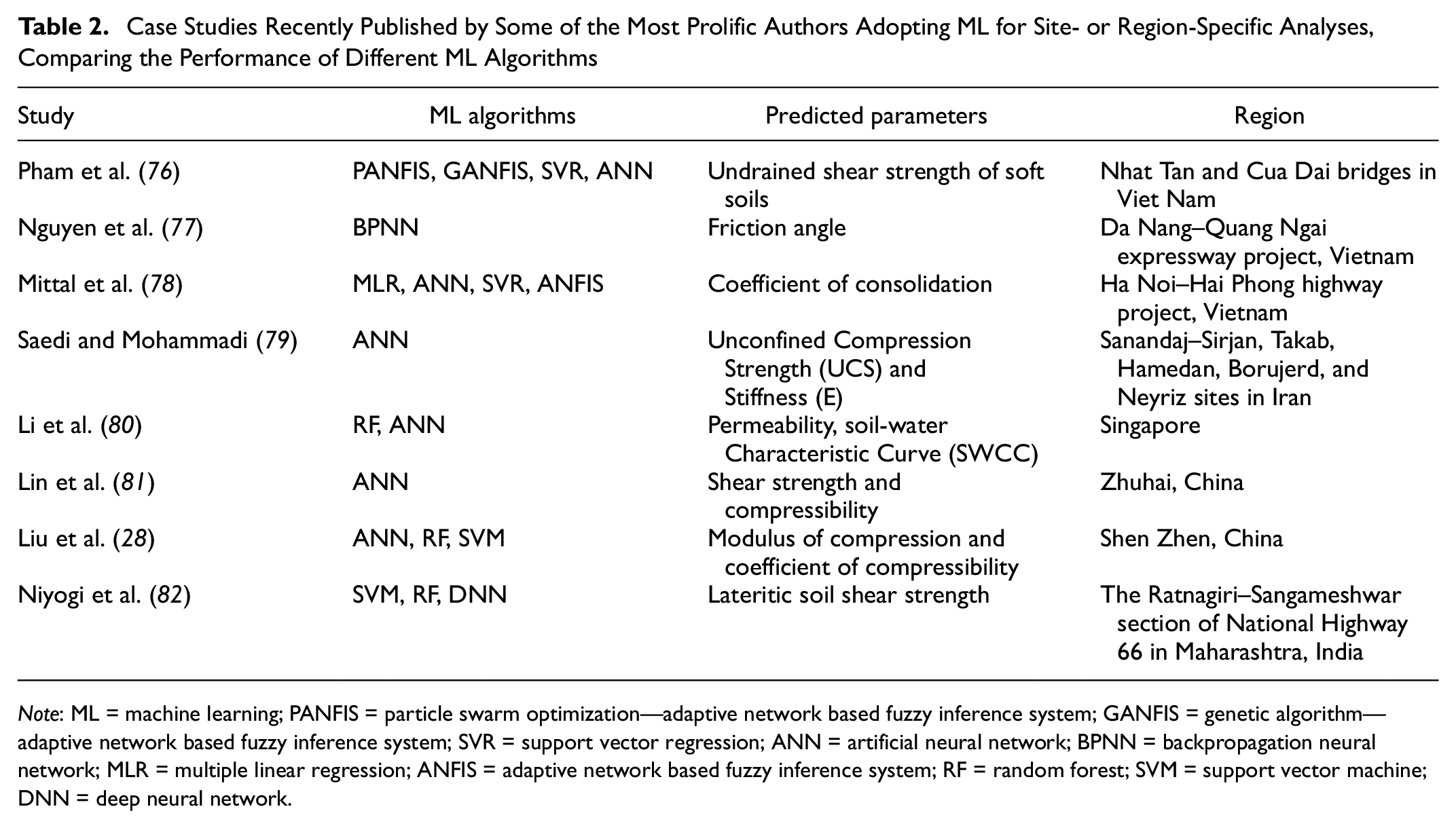
Note: ML = machine learning; PANFIS = particle swarm optimization—adaptive network based fuzzy inference system; GANFIS = genetic algorithm—adaptive network based fuzzy inference system; SVR = support vector regression; ANN = artificial neural network; BPNN = backpropagation neural network; MLR = multiple linear regression; ANFIS = adaptive network based fuzzy inference system; RF = random forest; SVM = support vector machine; DNN = deep neural network.
Different authors have employed different operational procedures to move from the construction of the database needed to feed the ML algorithms, to the prediction of the properties of geomaterials, and to the performance evaluation of the computational model. Three main common phases of analysis may be recognized in each procedure: 1) data preprocessing; 2) model building and validation; and 3) testing.
Step 1. Data Preprocessing
Data preprocessing facilitates the training process by appropriately transforming the entire training data set to remove outliers, produce the optimal set of input variables (features), and normalize different features to an equivalent range, which can be used to build an ML model. It is not surprising that outlier detection is not very often carried out as only a limited number of data points are available in most of the studies. Moreover, outliers can be hard to define for geo-properties. Among the few studies, Li and Misra ( 83 ) used isolation forest to remove outliers of compressional and shear travel time logs (DTC and DTS) acquired using sonic logging tools. Correlation analysis and feature selection is another important step in data preprocessing. It is vital to remove highly correlated input features and irrelevant features for the prediction of physical and mechanical properties. Correlation coefficients are widely used to measure the correlation between features, for example, the Pearson correlation coefficient and Spearman correlation coefficient. Various feature selection techniques can be used for removing irrelevant features, such as least absolute shrinkage and selection operator algorithm (LASSO), random forests—recursive feature elimination (RF-RFE), and mutual information have been applied by Mittal et al. ( 78 ). SHapley Additive exPlanations (SHAP) ( 84 ) was used by Li et al. ( 80 ) to investigate the impact of each input variable on different output soil properties. These indices could be used to validate the results, enabling researchers to explore the algorithm’s logic and verify its reliability.
Step 2. Model Building and Validation
As indicated in Table 2, most studies used conventional ML techniques, for example, ANN, SVM and tree-based methods. There is no consensus on a specific “optimal” ML algorithm for predicting physical properties of geomaterials. Pham et al. ( 76 ) concluded that out of four models the PANFIS emerges as a promising technique for prediction of the strength of soft soils. The ANN was the best model in Liu et al. ( 28 ), as it provided a simple analytical form with no hidden dependency between the bias and predicted indices. While building and testing the ML models, the entire data set is usually split into training and testing data sets. The training data set could be divided further into training and validating data sets, or the cross-validation techniques could be applied to a limited data sample, without further splitting of the training data set.
Step 3. Testing
The ML models established in Step 2 need further evaluation of their performance against unseen data sets. The common performance metrics that are typically adopted in the literature include:
expressions quantifying the error of the analysis by means of an objective function (OF), the coefficient of determination (R 2 ), the mean absolute error (MAE), and the root mean square error (RMSE);
the model bias method using bias mean, bias coefficient of variation (COV), and bias probability distribution ( 81 ).
Generic and Benchmark Data Sets
Site-specific data in geotechnical engineering are generally limited (from several hundred to a thousand at most). Therefore, data samples collected from various sources or places were used to develop ML models. It is worth mentioning that the database compilation by ISSMGE TC304 (304 dB) (http://140.112.12.21/issmge/tc304.htm) could be a suitable platform for using open data sets. Asghari et al. ( 85 ) and Zhang et al. ( 6 ) used the 304 dB to investigate the application of ML methods for the prediction of the undrained shear strength of soft soils and other complex correlations in engineering metrics. Ma et al. ( 86 ) developed hybrid GA-SVM and PSO-SVM models for the prediction of permeability of cracked rock based on a database developed from existing literature. Zhang et al. ( 87 ) investigated the performance of five commonly used ML algorithms, that is, backpropagation neural network (BPNN), extreme learning machine (ELM), SVM, RF, and evolutionary polynomial regression (EPR) in predicting compression index Cc based on a global database consisting of 311 data points of initial void ratio e0, liquid limit water content wL, and plasticity index Ip. Chen and Xue ( 88 ) collected a total of 151 data sets from the literature that were used to construct the ML models.
Uncertainty Quantification
Uncertainties associated with geomaterials (soils, rocks), geologic processes, and possible subsequent treatments are usually large and complex. Current ML modeling is always deterministic. As such, only high-quality data can be used because there is no capacity to address uncertainties. Zhang et al. ( 89 ) pointed out that applying the predicted result without any reliability evaluation using ML-based models may induce high risk. A Bayesian neural network (BNN) integrated with variational inference (VI) and Monte Carlo dropout (MCD) was used in their study to predict the compression index Cc and undrained shear strength su of clays and to evaluate the reliability of the ML model. An ANN-based model that takes into account uncertainty estimates was developed in ( 90 ). The database of CPTU and triaxial tests used contained 241 laboratory triaxial tests. All test specimens were of high quality, including 180 undisturbed specimens taken with a 72-mm diameter fixed piston sampler and 61 undisturbed specimens taken with 40-cm diameter block samples. The ANN model requires the water pressure and effective stresses in addition to the CPTU data. The standard deviation estimate was performed based on the “dropout method” described in Gal ( 91 ). The predicted and measured undrained shear strength in triaxial compression are compared in Figure 2. An estimated standard deviation of the predicted undrained shear strength is also shown.
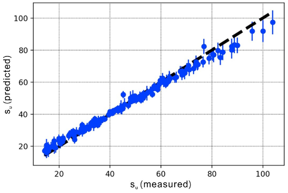
Predicted versus measured cone penetration test (CPT) undrained shear strength (in kPa) over the test data set. The vertical line shows the estimated standard deviation. The black dashed line is the 1:1 line.
3-D Integrated Ground Model
For large geotechnical projects on land and offshore developments, it is current practice to conduct both geophysical and geotechnical investigations. Ground models integrate the geotechnical and geophysical data collected from a site and provide a three-dimensional map of the stratigraphy and the geo-properties.
In geotechnical projects, the quantitative integrated ground model is a requirement for cost-optimal site characterization. The ground model refers mainly to the stratigraphic configuration and the associated geotechnical properties in this study. Extensive studies focusing on the stratigraphy classification or the geomechanical characterization have been reported in the geotechnical literature (e.g., Mariethoz and Caers [ 34 ], Shi and Wang [ 47 ], and Wei and Wang [ 72 ]). However, relatively limited studies dealt with both the stratigraphic configuration and the geomechanical parameters in a specific model ( 92 ). Note that both the strata and the geo-properties at a site are a product of the same deposit histories, tectonic, and human activities; their spatial distributions are expected to share similar features. Thus, the study on the site characterization that considers both the stratigraphy classification and the geomechanical characterization, especially the spatial variabilities of the stratigraphic configuration and the associated geotechnical properties, is warranted.
In the conventional engineering approach, the subsurface stratigraphic configuration at a site is usually constructed through spatial interpolation of the stratigraphy collected at borehole locations, coupled with local experience ( 51 ). The geo-properties of each stratum are taken as fixed values (e.g., the mean of the geo-properties derived at borehole locations) ( 93 ). The ground model constructed with the conventional approach simplifies the actual geological body. Although this conventional approach has been widely adopted in practice, no scientific rationale is available to support this simplification ( 92 ).
Geotechnical analyses and interpretations often rely on isolated 1-D boreholes. On the other hand, geophysical data are collected in 2-D lines and 3-D volumes. Geophysical data therefore provide the natural link to repopulate geotechnical properties found in the 1-D boreholes onto a larger area and thereby build a consistent and robust ground model ( 94 ). Thus, it is current practice to conduct both geophysical and geotechnical investigations for large geotechnical projects on land and offshore developments. Ground models integrate the geotechnical and geophysical data collected from a site and provide a 3-D map of the stratigraphy and the geo-properties. Many approaches, such as the geometrical approach ( 94 ), the geostatistical approach ( 95 ), and the ANNs ( 96 ) have been reported to map the dynamic properties from the seismic data (stratigraphic information, P-wave velocities, amplitudes, and their attributes) into the geotechnical or geomechanical properties. Sauvin et al. ( 94 ) showed that the machine learning approach provides the most accurate prediction of the ground model from the geophysical data, over the geometrical geostatistical approach and the geostatistical approach.
The implementation procedures of the machine learning approach presented in Mittal et al. ( 78 ) can be summarized as follows.
Step 1. Derive a range of quantitative attributes from the seismic reflection data, particularly acoustic impedance using a genetic algorithm for optimization.
Step 2. Convert the seismic attributes from the time domain into the depth domain.
Step 3. Down-sample the piezocone penetration test (CPTU) tip resistance (qc) to a sample interval matching that of the depth-converted seismic attributes.
Step 4. Use an ANN to perform multi-attribute regression between the range of quantitative seismic attributes and CPTU qc by training at several calibration sites.
It is worth noting that above approaches focused on deriving the most-probable ground model; however, the spatial variabilities of the stratigraphic configuration and the associated geotechnical properties were generally ignored. To overcome this obstacle, Shi and Wang ( 97 ) proposed a stochastic framework for modeling the stratigraphic uncertainty and spatial variability of soil properties by machine learning and random field simulation from limited site investigation data. This framework could effectively generate multiple realizations of geological cross-section and random field samples of geotechnical properties from limited measurements (obtained from the CPT), through which the uncertainties associated with the ground model can be characterized. We recommend the proposed framework for characterizing the ground model and associated uncertainties.
Step 1. CPT-Based Soil Classification and Interpretation of Consolidation Parameters
The cone penetration test (CPT) is a commonly used in situ testing method for soil classification and characterization of subsurface geotechnical property profiles. CPT provides direct continuous vertical line measurements of cone pressure, sleeve friction, and pore pressure. Apart from soil classification, CPT data can also be used to estimate the soil properties of fine-grained materials via empirical correlations established in the literature (e.g., Robertson and Cabal [ 98 ]).
Step 2. Stratigraphic Uncertainty Modeling by IC-XGBoost2D
The iterative convolution extreme gradient boosting (IC-XGBoost2D) is a stochastic simulation algorithm for developing 2-D subsurface geological cross sections from training images and limited site-specific measurements. A training image reflects prior geological knowledge at the area of interest and serves as an effective supplement to limited site-specific data ( 99 ).
Step 3. Modeling Soil Property Spatial Variability from Limited Measurements
Bayesian compressive sampling (BCS) is a non-parametric machine learning method developed for interpolating spatially varying geo-properties (e.g., cone pressure) from sparse measurements. Under compressive sensing/sampling, a complete signal (e.g., 2-D spatially varying soil property profiles) can be approximated as a weighted summation of a limited number of pre-specified basis functions (e.g., discrete cosine basis functions).
Step 4. Sequential Modeling of Soil Property Spatial Variability for Each Soil Type
Once subsurface geological cross sections or realizations are developed using IC-XGBoost2D, the best estimate of cone pressure, sleeve friction, and pore pressure within the 2-D cross section with high spatial resolution can be obtained using BCS and CPT measurements.
Scour Assessment Using ML
Various recent studies have looked into applications of AI-ML in geohazard assessment and management for geotechnical systems ( 100 , 101 ). In this paper, we focus on scour as one of the most critical mechanisms affecting bridge foundations and how ML techniques can be implemented step by step to provide more reliable bridge scour estimation and real-time risk assessment for design and maintenance purposes, respectively.
In the past two decades, numerous studies have explored local scour prediction around bridge piers using ML. SVM, genetic algorithms ( 102 , 103 ), and artificial neural networks (ANNs), particularly FFNN or multilayer perceptrons (MLP) ( 104 – 107 ) are among the most commonly used techniques. These ML methods have shown superior performance over traditional empirical equations in the accuracy of maximum scour depth predictions for a given training data set; however, the generalization ability of these types of predictive models decays significantly outside the convex hull of the training data set, which can lead to poor generalization to unseen data ( 108 ). Therefore, to use these models for maximum scour depth prediction, the bridge characteristics must be within the training database range. A good review of the literature can be found in Sharafati et al. ( 109 ).
Given the limitations of the current scour prediction models, the complexity of scour phenomenon, uncertainty in flow (flood levels), riverbed and geomorphological conditions, real-time monitoring, and forecast to manage the scour risk is evolving as a promising tool. Yousefpour et al. ( 107 , 108 ) have pioneered this approach by using historical monitoring data from bridge piers, including timeseries of scour depth and river flow depth variation. In their approach, they have used both DL and Bayesian inference methods that have shown reasonable accuracy in providing real-time assessment of scour depth. In their most recent study, they have developed long short-term memory (LSTM) models that can provide estimates of scour depth a week in advance for case study bridges in Alaska ( 108 ).
Based on a critical review of the existing methods, the following techniques are recommended for maximum (design) and real-time scour depth prediction (maintenance).
Maximum Scour Depth Prediction Using Feed-Forward Neural Networks
Fully connected FFNNs or MLPs are powerful in representing nonlinear high dimensional processes influenced by multiple physical factors. MLPs are universal approximators theoretically capable of approximating any function, even with only one hidden layer with enough nonlinear computational units (neurons) ( 110 , 111 ).
The application of FFNNs in developing scour prediction models has been explored by numerous studies, as referenced in the previous section. Many used the US National Scour Study database developed by the US Geological Survey (USGS) in collaboration with the Federal Highway Administration (FHWA) ( 1 , 2 ). However, these models can hardly be used in mainstream scour design. The major obstacles in upscaling such ML models to practice are:
1) Poor generalization/extrapolation capacity: This is a result of the dependency of ML models on the range of training data, meaning ML models need to be trained with a database that is statistically representative of a particular bridge.
2) Database deficiencies and poor statistical design: Databases are built with stitching scattered data sets without much statistical design, involving many variables that show sparse range across the various data sets.
3) Errors and subjectivity in measurements: This issue with scour depth measurement requires a judgment on the reference surface. Different judgments/assumptions on reference levels such as ambient bathymetric, as-built, or maximum bed levels can result in different reported scour depth in field measurement data. For more information, refer to Landers and Mueller ( 1 ).
4) ML knowledge and implementation complexities: Lack of ML (and coding) knowledge and experience in practice engineers, along with a lack of guidelines, hinder AI-ML application for bridge scour design.
The following methodology is proposed to develop a simple ML model to estimate the maximum scour depth with a confidence bound for a new bridge. For more details on the approach, readers are referred to Yousefpour et al. ( 107 ). Engineering due diligence and quality control checks must be taken when applying this method for design:
Step 1. Database Compilation
Using the USGS National Bridge Scour Database, a “global” ML model can be trained first. This model needs to be later retrained (transfer learning as explained in step 2) using a “local” or site-specific database with a well-designed statistical distribution. The local database should include data from several bridges with relatively similar riverbeds, flow, and structural characteristics. The key input/target parameters for the scour ML model are listed below, as identified in many earlier studies. These parameters for the new bridge should lie in the convex hull of the local database for a reliable scour prediction:
Input parameters (features)
Sediment transport (scour type): This can be divided into live-bed or clear-bed. In clear-water conditions, there is limited transport of bed material into the channel from upstream, whereas, in live-bed conditions, materials are transported through upstream flow and deposited downstream (filling after scour). For more details on the definition, refer to Landers and Mueller ( 1 ) and Mueller and Wagner ( 2 ).
Flow depth: This should be measured using gauges, stage sensors, or other techniques. For best practice in the measurement of such parameters, readers are referred to Mueller and Wagner ( 2 ).
Flow velocity: Acoustic doppler velocimeters (ADV) can measure average velocity around piers. For best practice in velocity measurements, readers are referred to Landers and Mueller ( 1 ).
Pier/pile geometry (shape, skew, width, and length): This is available in national databases (US National Bridge Inventory [NBI]) and can be measured on site or extracted from bridge plans/drawings.
Bed condition: This determines the cohesive or non-cohesive nature of sediments around the bridge.
Sediment size: Median grain size (D50) can be measured from sampling at the site or from bridge design site investigation reports. The common sampling methods are explained in Landers and Mueller ( 1 ).
Target parameter (output)
Scour depth: This should be measured after a flood event—within 24 to 48 h in a live-bed scour situation (mostly observed in non-cohesive river beds); this allows reaching to equilibrium scour depth. For clear-bed scour the time-dependency of scour needs to be established to determine the suitable time of scour depth measurements.
The key point in this step is to develop a statistically well-designed database that can be representative of the population of bridges in a region of interest. The importance of the statistical design of databases is seemingly overlooked in the current literature, especially given the surge of featureless DL approaches. By referring to core statistical knowledge, we know that the skewness of a database (especially for smaller data sets) can lead to the model favoring specific parameters and trends in the data (bias), which results in unreliable predictions. To have a well-designed database, the statistical distribution of all parameters in the database should be analyzed to ensure that there is a relatively uniform distribution across the range of variability. The data should be normalized before training the ML model.
Step 2. Developing a “Simple Enough” ML Model
A simple MLP (FFNN) network is shown in Figure 3. A three-layer architecture, with one hidden layer applying a sigmoid activation function such as the ones explained in Yousefpour et al. ( 112 ) can be followed. For regression problems, using more than one layer and too many units often does not lead to more accurate predictions. For theoretical details of MLP algorithms, readers are encouraged to refer to Hornik ( 110 ). Training in MLPs means adjusting the weights and biases to reach the universal minimum of a loss function, which is usually defined as the mean of squared prediction errors (MSE) across the training database. However, more often than not, optimization techniques find a local minimum instead of the global minimum. Several techniques can be implemented to avoid being trapped in a local minimum, such as regularization, cross-validation, and early stopping, among others. A practical method is early stopping based on a “patience number,” which is the maximum consecutive number of times to allow the error to increase over a validation data set during training ( 113 , 114 ).
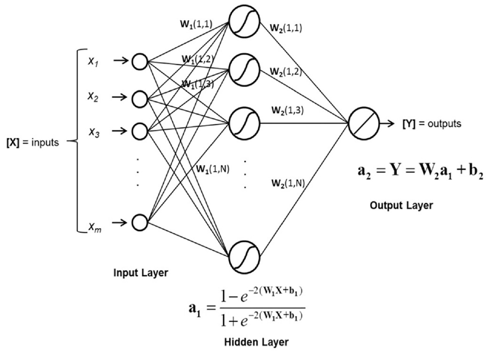
Simple architecture for MLP/FNN ( 3 ).
The generalization of ML models is assessed based on a test data set, which represents the model performance on unseen data. Several metrics can be used for this purpose, including RMSE, coefficient of determination (R 2 ), MSE, and MAE. MAE and RMSE allow error measurement in the same unit as the target parameter.
Transfer learning has been proven to improve the performance of ML models significantly ( 115 ). In this method, instead of training an ML model from scratch, that is, starting from a random point in the space of weights and biases, the model is initialized using a set of parameters from a previously trained model. In the context of image data and pattern recognition, this can have a tremendous effect; therefore, using pre-trained models is a must. In the context of scour prediction, this can mean “transferring the learning” from a model trained using a global database of scour to a site-specific ML model that needs to be trained with a local database.
For this purpose, first a “global ML” model can be trained according to the recommendations in step 1, then a “local ML” can be trained, initializing from the set of weights and biases of the trained global model.
Step 3. Validation and Fine-Tuning
Using an ensemble of models provides more accuracy in predictions and enables uncertainty assessment. An ensemble of FFNN can be generated by repeating (random initiation of network weights and biases) the training over many times (+50) to find a group (ensemble) of best models. The ensemble’s performance can be reported by using first-order statistics of the resulting distributions. Readers are referred to Yousefpour ( 3 ), Bateni et al. ( 104 ), and Sagi and Rokach ( 116 ) for more details on ensemble methods.
One of the most effective cross-validation techniques that also can be integrated with the ensemble method, is to use K-fold or Monte Carlo cross-validation ( 117 ) (as opposed to the hold-out method) to enable making the most out of a small database. In this technique, the networks in the ensemble use various parts of the data for training, validation, and testing, as shown in Figure 4.
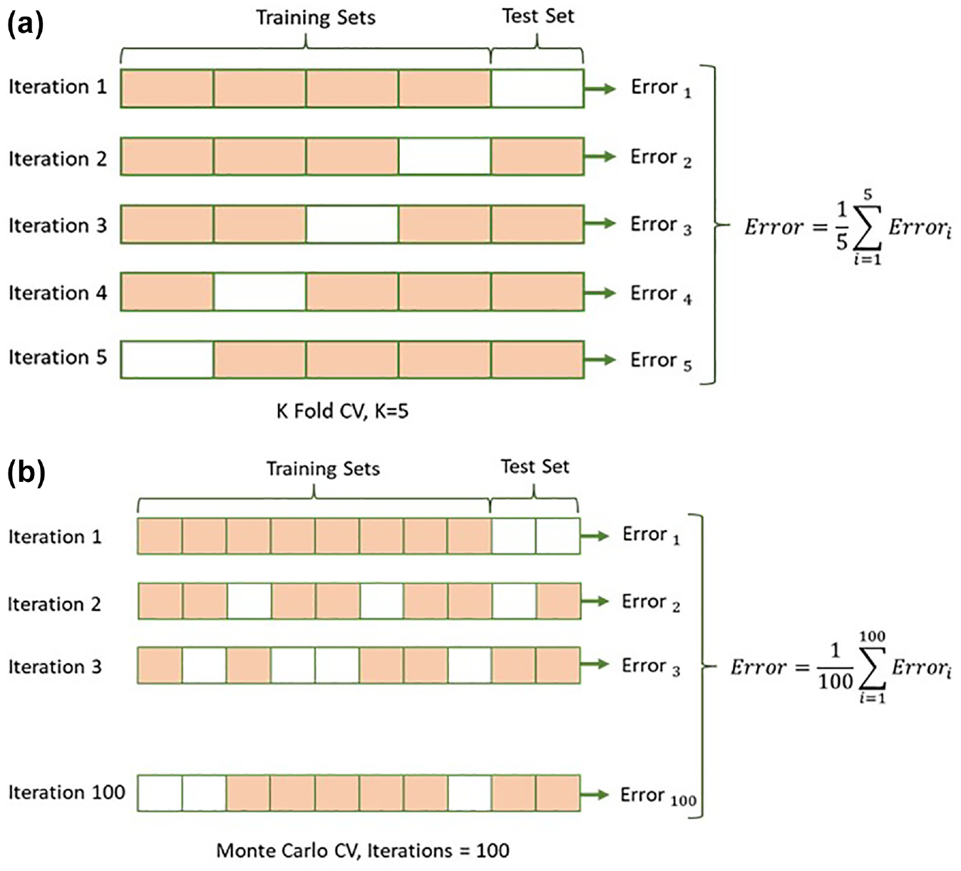
Cross-validation methods: (a) K-Fold; and (b) Monte Carlo.
Fine-tuning and hyperparameter optimization can lead to superior network configurations. The main hyperparameters for an FFNN model include the number of hidden layers, the number of units in each hidden layer, the type of activation function in units, input feature selection/combination, optimization, and training parameters such as learning rate, maximum number of epochs, and early stopping criteria (patience number, minimum error, etc.). The most commonly used hyperparameter search techniques are grid-search and random search, which can be applied to speed up the optimization process ( 108 , 118 ). Several available codes and libraries in Python can be readily applied, such as Optuna and Talos ( 119 ).
Step 4. Assessment of ML Predictions
The ensemble of the best FFNNs generates a distribution of predictions on scour depth for a given bridge. Having a larger ensemble ensures the uncertainty is better captured. Mean, standard deviation, and 95% confidence bound can be reported from the generated distribution. We recommend scatter-plotting the scour depth versus velocity and flow depth for all the records in the local database and locating where the ML prediction lies within the local and global database. The ultimate judgment on the scour depth estimates for a given bridge at a target flood level (e.g., 200-year return period), needs to be based on both the ML prediction and the historic local trends observed from past flood events.
Real-Time Scour Assessment Using Deep Learning
Regular inspection and monitoring of the scour in existing bridges has been mandatory in the United States and some other countries because of frequent catastrophic events in the past few decades caused by scour failure of bridges. Scour is the most common cause of failure for bridges, with approximately 260,000 scour critical bridges across the country ( 120 ).
Given the shortcomings in scour depth estimation with existing methods, many bridges are highly vulnerable to scour. The US NBI has identified the scour risk of all bridges in the United States with a “scour-vulnerability” index ( 121 ). This index is assessed based on regular scour inspection and monitoring mandated by FHWA.
Real-time monitoring for bridges exposed to a higher risk of scour can enable reliable risk management and a data-driven understanding of scour process. Several US Departments of Transportation (DOT) in partnership with USGS have started rigorous scour monitoring programs for their most vulnerable bridges. States such as Alaska, with most bridges exposed to seasonal flooding, started this program in the early 2000s (available at Alaska Science Center). Other states such as Idaho, Colorado, and Oregon, have followed similar approaches. This monitoring program allows for real-time measurement of bed elevation and flow level at a bridge pier using sonic/echosounder devices (see Figure 5) that measure the distance based on the sonic wave travel time within a specific material (water or air). For more details, readers are referred to USGS published reports for each state ( 122 ).
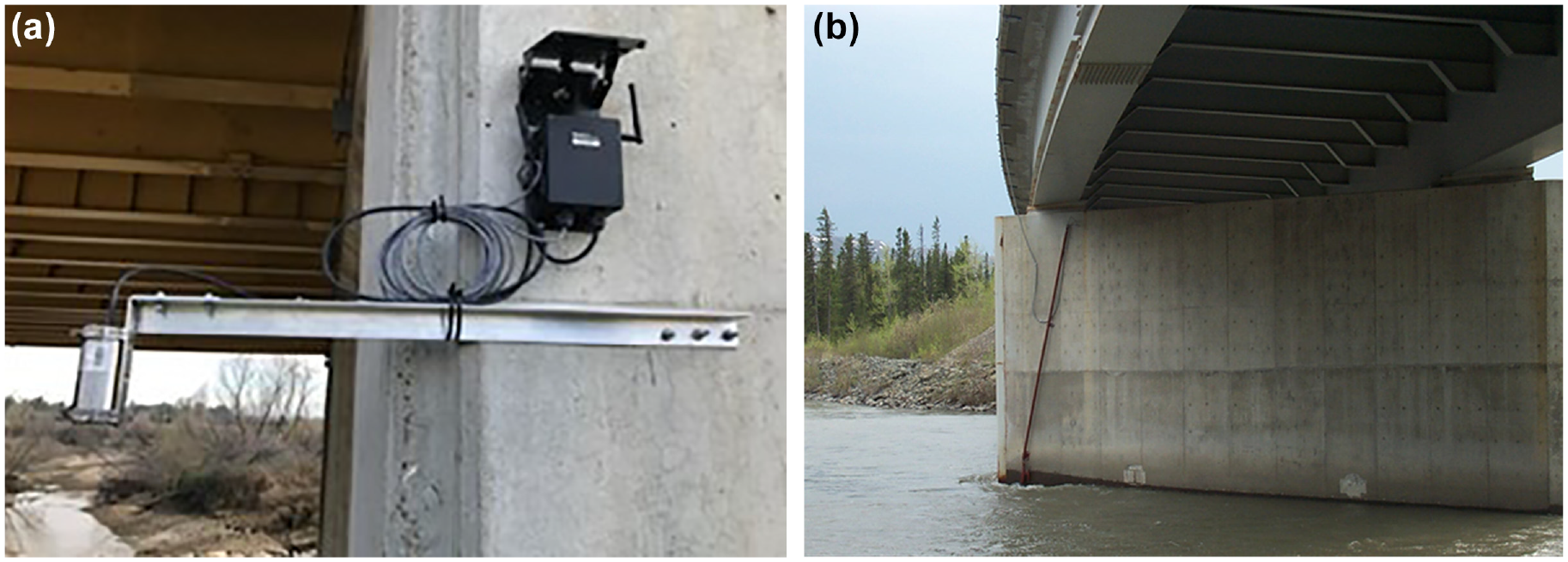
Sensors mounted on bridge piers in California and Alaska for continuous measurement of river water and bed elevation: (a) solar-powered stage; and (b) sonar.
Yousefpour et al. ( 107 , 108 ) studied the historic Alaska monitoring data in their recent research to develop scour forecast and early warning models using DL methods. They have proposed an AI-based methodology for real-time scour assessment to enable more reliable risk assessment for critical bridges. The DL models can also provide insights into estimating the maximum scour depth for new bridges within the same region with similar flow, structure, and characteristics. The proposed methodology can be implemented for the assessment of scour in existing bridges as per the following steps:
Step 1. Collecting Site-Specific Historic Scour Data: Continuous Measurement of Bed and Flow Level (and Velocity) Variation
A review of existing scour field monitoring data can be found in Hunt ( 123 ). Despite the challenges of sensor readings, which may result in missing data across a year, such as sensor damage resulting from flooding, accumulation of trash and debris, and vandalism, they can provide valuable information about the scour process for a particular bridge. The generated timeseries data of flow depth and scour depth enable site-specific scour assessment, which can be powerful in addressing the “extrapolation” problem of ML models discussed in the previous section.
Any type of sensor that can continuously measure flow and bed levels can be instrumental. The measurement of bed elevation measurement using sonar sensors is well explained in Henneberg ( 124 ). Current methods for measurement of flow level or stage are explained in Sauer and Turnipseed ( 125 ). Flow velocity measurements are also recommended, which can be measured by acoustic doppler and velocimeters as described in Sauer and Turnipseed ( 126 ).
Step 2. Data Processing
Data processing is a vital step before ML development. Although DL models have been proven to be powerful in addressing noise and outliers in training data ( 108 , 118 , 127 ), performing the following processing can enable faster learning and more reliable performance:
1) Basic cleaning and synchronization of timeseries: For scour sensor data, that could mean ensuring random errors in data are removed and ensuring a reasonable resolution (reading intervals) for all timeseries data and synchronizing the readings among various sensors, such as bed elevation, flow elevation, and velocity. Down-sampling and up-sampling can be performed to ensure the data are captured with reliable resolution. For scour, half-hourly or hourly readings are recommended as scour and flooding can develop within a few hours.
2) Outlier detection: Detecting outliers is essential as it can mislead the model with seemingly correct but erroneous readings. Figure 6 shows an example of how accurate outlier detection can affect identifying the true trend of the scour data. One of the common methods for outlier rejection is the median absolute deviation (MAD) method. Data is first normalized (standard normal) and points with absolute values greater than 3.5 are defined as outliers within a selected time window. The length of this window is critical and needs to be adjusted depending on reading intervals and expected time variations in the data. For instance, variation in scour depth (in case of live-bed scour) can happen within a few hours to a few days. MAD is more robust than traditional standard deviation methods and less sensitive to outliers and extremes.
3) Missing data imputation: This is very common for scour data resulting from blockage of sensors by debris accumulation or flood-related disturbance, among other reasons. Therefore, applying emerging imputation techniques in cases where the available data is sparse but nevertheless valuable in understanding the scour trend is essential. Moritz and Bartz-Beyerstein ( 128 ) provide an overview of univariate timeseries imputation techniques. One of the simplest methods is linear interpolation and more advanced methods, such as the Gaussian process can enable more realistic data representations ( 129 ).
4) Smoothing and filtering: Moving average and other auto-regressive methods can be quite powerful for timeseries smoothing and denoising ( 130 , 131 ). They have specifically been found useful for sonar and stage sensor data (171). Signal processing methods such as the low-pass filtering technique can enable removing extreme frequency ranges from the data. Figure 7 shows how these different methods compare for sonar data from a bridge in Alaska.
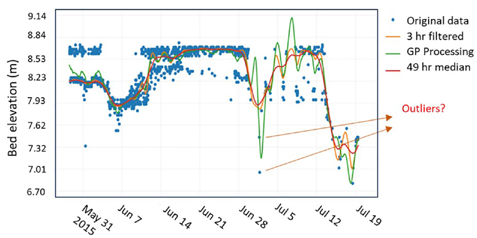
Outlier detection in sonar (scour) data, comparing various denoising and filtering techniques.
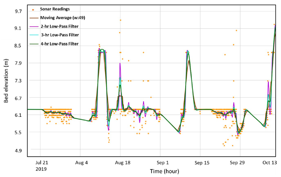
Comparing various filtering/smoothing methods for sonar timeseries data.
Step 3. Developing DL Models: LSTMs and CNNs
In RNNs, the output of each neuron goes back to itself, and the units in the subsequent layer at each time step. This enables these algorithms to keep a “memory” of past “activations.” LSTM networks are particular types of RNN that use special “gates”—input, forget, and output gates—to update the memory state at each step, as shown in Figure 8 ( 132 ). This enables LSTMs to maintain a short and long-term memory of temporal patterns within timeseries data and incorporate them into future predictions. LSTMs have shown superiority compared with other RNNs for timeseries forecasting in various fields, owing this success to their ability to overcome the problem of vanishing gradients ( 133 ).
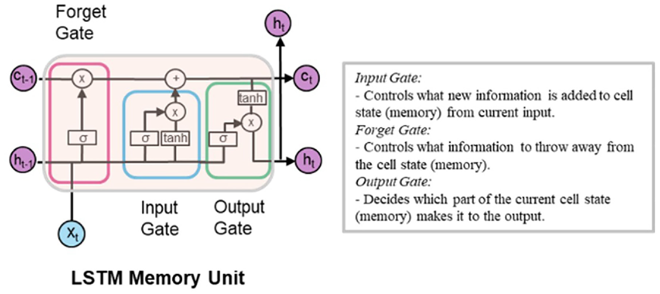
Long short-term memory (LSTM) unit-showing details of input, output, and forget gates; x t = input feature at time step t; c t = cell memory state; h t = hidden state or output at time step t; σ = sigmoid activation function; tanh = hyperbolic tangent function ( 108 ).
For scour forecasting, Yousefpour and Correa ( 108 ) showed that LSTM can provide far more accurate predictions of scour compared with empirical equations. In their case studies on Alaskan bridges, they developed three variants of LSTM algorithms that can provide scour prediction seven days in advance with an average error of 0.2 to 0.35m. In a more recent study, they explored applying CNNs as a more computationally efficient DL algorithm for real-time forecast of scour, and compared CNN and LSTM performance on data from Alaskan bridges ( 118 ). Results showed competitive performance by temporal CNNs with significantly lower computational cost. Figure 9 shows the LSTM and CNN architectures used in these studies for sonar timeseries prediction.
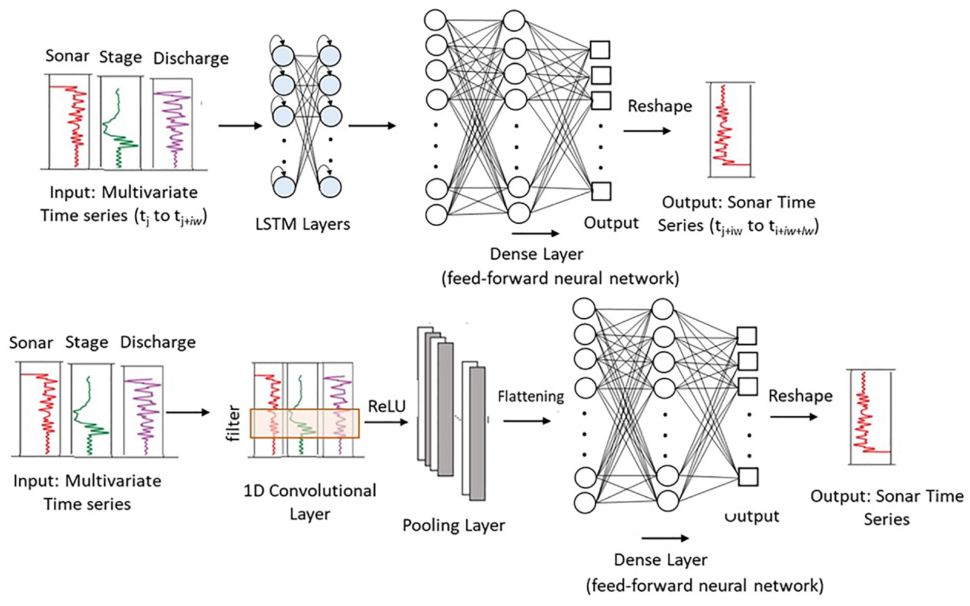
Architectures of networks for scour forecast: (a) LSTM; and (b) CNN: iw = input width; lw = label (output) width of a data slice ( 118 ).
The training of DL models is done by timeseries sequences generated by slicing the whole timeseries data into smaller sequences (data slices) using a sliding window. This process is explained in detail in Yousefpour and Correa ( 108 ). The sliding window moves over the database one timestep at a time. Each sequence (data slice) has an “input” and a “target” or “label” segment, as shown in Figure 10. The training is done in batches containing several data slices. The network’s weights and biases are adjusted like MLPs by minimizing the error of prediction over the label length of data slices.
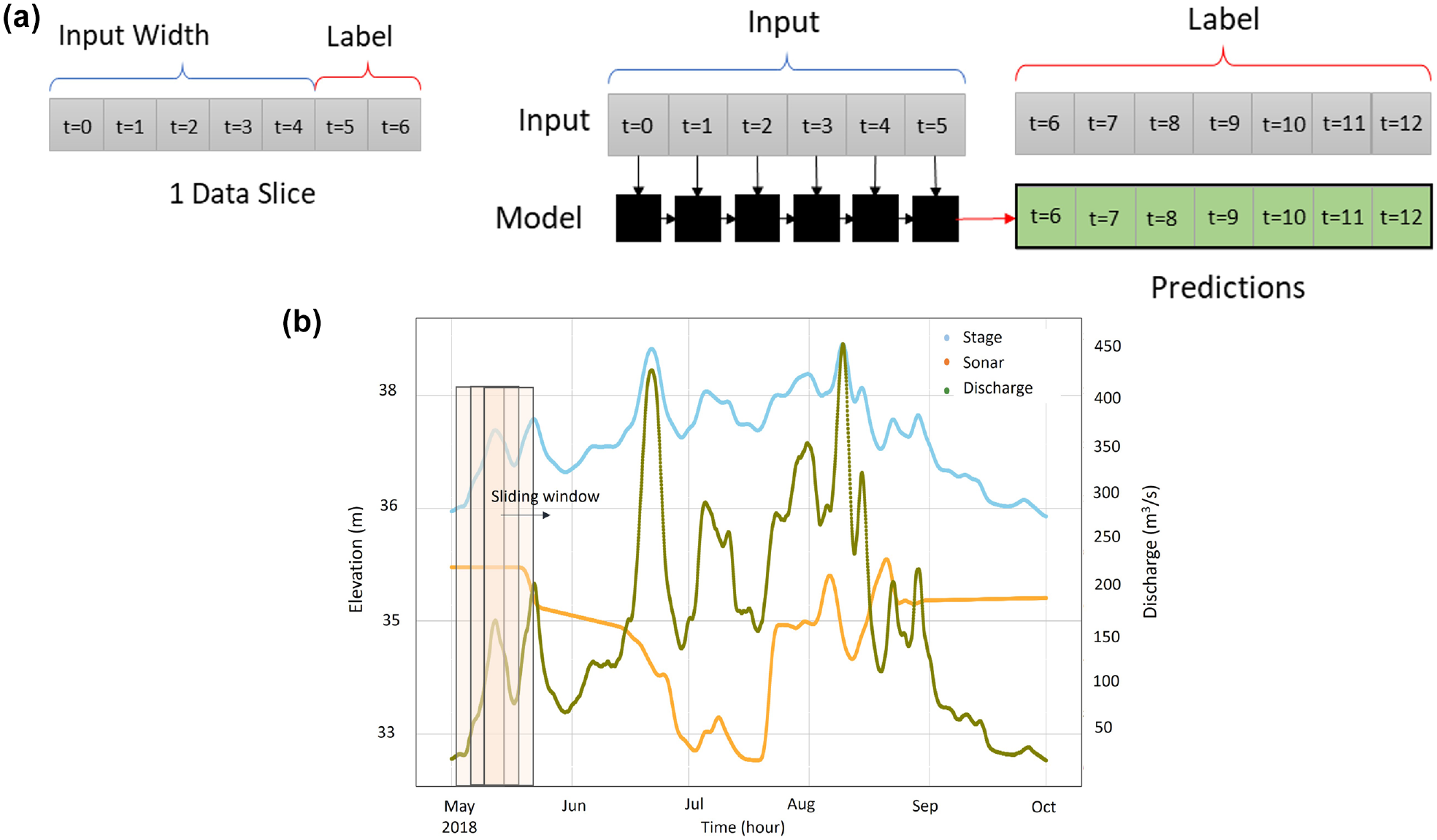
Data slicing for scour timeseries forecasting with deep learning (DL): (a) example of a data slice (sequence) and how it is fed into a DL model; and (b) slicing the timeseries data using a sliding window, including input plus label sequence.
Step 4. Fine-Tuning and Validation of DL
To obtain the optimal configuration of these DL algorithms, hyperparameter tuning must be performed, similar to what was recommended for FFNNs in the previous sections. One important hyperparameter in timeseries forecasting is the input and label width and their ratio. The impact of selecting the most optimal sequence length to ensure the temporal variations in the data are well explained in Yousefpour and Correa ( 108 ) and Yousefpour and Pouragha ( 134 ). The label width is the length of forecast window and should be selected to provide enough time for implementing proper risk countermeasures. In case of bridge scour, a minimum of seven days was deemed necessary.
Cross-validation methods similar to FFNNs can be implemented to improve the performance of the DL models and reduce the chances of overfitting. One crucial difference is the temporal dependencies in timeseries data, which can make data division for training a bit absurd. We recommend ensuring that training, validation, and testing are consecutive unless time is introduced as an additional feature to the models. Methods such as K-fold cross-validation can be implemented sequentially, as shown in Figure 11. In this method, the model is retrained at each step using transfer learning; the test data set in each step needs to be free of overlaps with the previous step data to avoid evaluating the model over “seen” data. A hold-out test data set can be kept aside to evaluate the final model at the end of sequential training. This metric can be compared and reported with the average performance of models over test data sets across the sequential training steps.
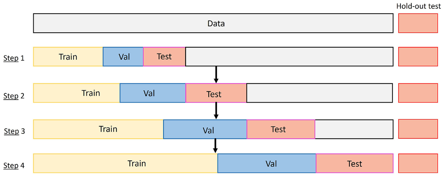
Sequential K-fold cross-validation with transfer learning: the arrow shows transfer learning between training steps.
The prediction of the DL model over data slices that have continuous overlaps results in overlap in predictions which will provide an uncertainty assessment opportunity. In addition, repeating the training several times provides a range of predictions that can be included in the set of predictions. Based on that, confidence intervals and the meaning of predictions can be established. Figure 12 shows an example of an LSTM and CNN model prediction over a test subset for an Alaskan bridge ( 118 ).
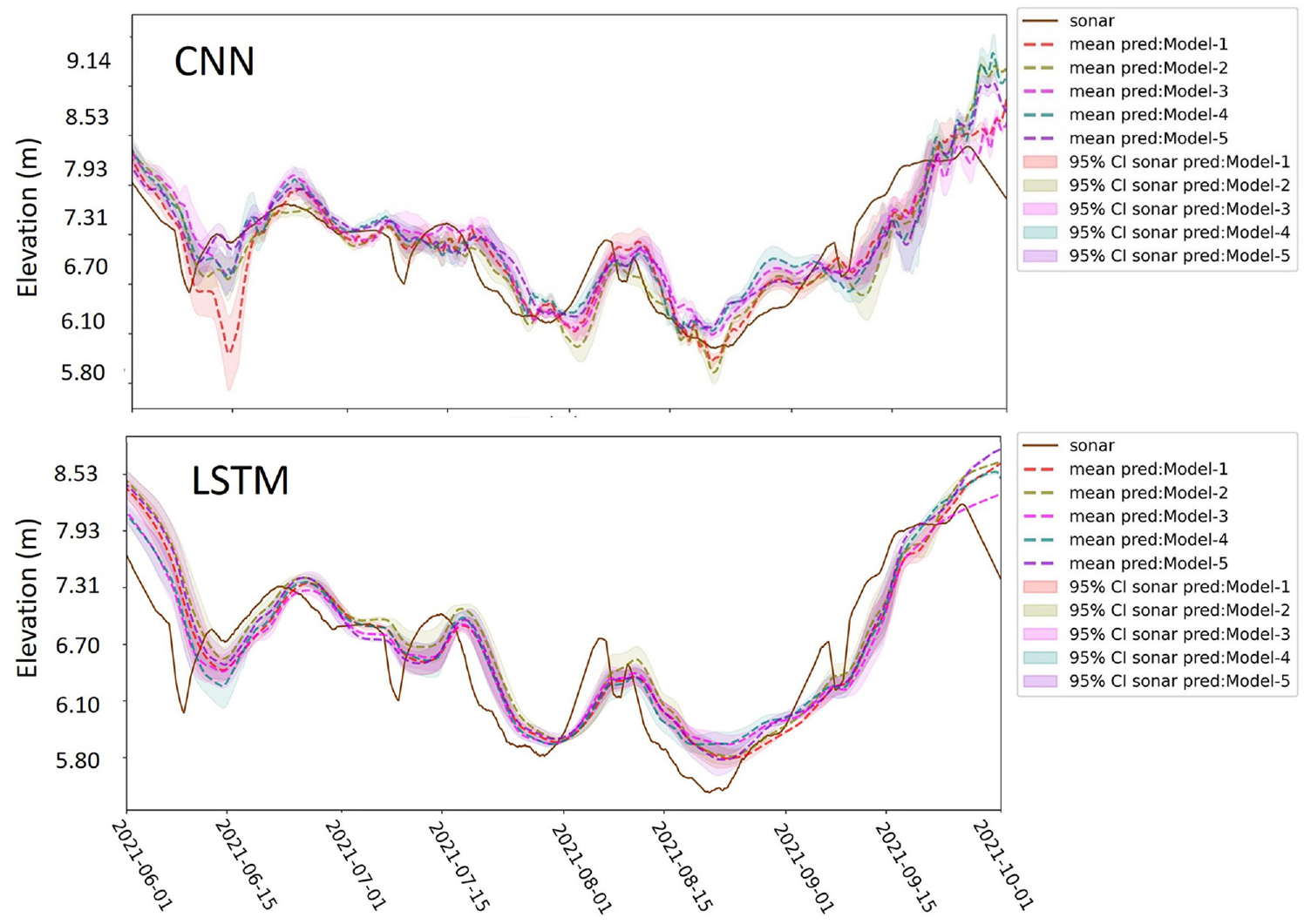
Scour forecast (seven days in advance) over a test subset of data (June to Oct, 2021) from the top five best LSTM and CNN models ( 118 ).
In addition to metrics of average error (MSE, MAE, or RMSE), the DL model predictions should be evaluated for trend detection, that is, peaks and troughs through fill and scour episodes. The error in prediction of peaks and troughs can provide another performance metric for the scour forecast model performance (read more in Yousefpour and Correa [ 108 ]).
Step5. Assessment of Upcoming Scour
The proposed real-time DL forecast models can provide a tool for risk assessments of an upcoming scour event. The uncertainty and reliability of the forecast must be assessed using engineering judgment by also evaluating meteorological and flood forecasts and the available historical trends for a particular bridge and/or similar bridges in a region. Lower bounds of scour depth predictions are recommended to minimize risk in detected major scours. Using real-time cameras or aerial photography (e.g., drones) can provide further inputs for more reliable decision making and taking the most appropriate plans of action to manage scour failure risks.
Conclusions
This paper discussed emerging AI-ML techniques for subsurface site characterization and geohazard assessments. Our review revealed that ML can be a promising solution for characterizing subsurface conditions and geomaterials. ML algorithms make more accurate predictions than traditional empirical correlations, while the interpretation and explanation of ML models need to be regarded as a secondary objective. There is no consensus on an “optimal” ML/DL algorithm for subsurface site characterization, even when looking at the results of the most recent comparative studies in the prediction of physical and mechanical properties of geomaterials. The choice between adopting conventional ML (ANN, RF, SVM, etc.) or DL algorithms primarily depends on the type and quantity of available data and if explicit expressions are preferred. The uncertainty associated with subsurface features (layer boundaries, discontinuities, voids, anomalies, etc.), spatial variability of geo-properties and ML modeling is another issue that needs further exploration. In the assessment of geohazards, bridge scour was the focus of this paper; nevertheless, the reviewed and recommended techniques can be applied to other types of geohazards. A step-by-step methodology for implementing both traditional ML and emerging DL methods was discussed in application to prediction and real-time forecasting of scour for bridge foundations. The guidelines and provided references can pave the way for implementing similar ML methods in practice. Some of the obstacles and challenges of applying these methods were also highlighted.
Footnotes
Acknowledgements
We acknowledge the contribution of Fatemeh Safari Honar in preparing the figures for this paper.
Author Contributions
The authors confirm contribution to the paper as follows: study conception and design: Negin Yousefpour, Zhongqiang Liu; data collection: Negin Yousefpour, Zhongqiang Liu, Chao Zhao; analysis and interpretation of results: Negin Yousefpour, Zhongqiang Liu, Chao Zhao; draft manuscript preparation: Negin Yousefpour, Zhongqiang Liu, Chao Zhao. All authors reviewed the results and approved the final version of the manuscript.
Declaration of Conflicting Interests
The author(s) declared no potential conflicts of interest with respect to the research, authorship, and/or publication of this article.
Funding
The author(s) disclosed receipt of the following financial support for the research, authorship, and/or publication of this article: Funding for this publication is provided by the Norwegian Geotechnical Institute, Oslo and the University of Melbourne.