Sage Journals: Discover world-class research

Abstract

This work aims to assess the occlusion of traffic signs for autonomous vehicles (AVs) using point cloud data, while addressing the limitations and recommendations of previous studies. Dense point cloud data are used to create a digital twin of existing roads and simulate a set of AV sensors within this environment. Convex polyhedrons or hulls with an octree data structure and semantic segmentation were used to assess traffic sign occlusion. Using the developed method, several case studies are presented to identify locations with occluded traffic signs for AVs. This work can help infrastructure operators and AV professionals make data-driven decisions about smart physical infrastructure investments for AVs.

Keywords

highway maintenance roadside maintenance operations roadway design geospatial data acquisition technologies lidar traffic control devices traffic signs

Significant progress has been made in autonomous vehicle (AV) development over recent years ( 1 , 2 ). While there is a lot of interest in, and research on, such technologies in the AV market, government bodies have been slow to assess the ability of current road infrastructure to accommodate these vehicles. In the United States, the Department of Transportation has conducted assessments of highways to prepare for the mass deployment of AVs ( 3 ). Similarly, Transport Canada has funded research on the effect of driverless vehicles on road infrastructure ( 4 ). The complete deployment of AVs will be gradual over the years. A classification of automation levels was created ( 5 ) to identify the transition from no driving automation (Level 0) to full driving automation (Level 5). Given that current roads are designed based on human driver constraints, it might be necessary to adjust them for vehicles with different automation levels as technology evolves ( 6 – 8 ). During the transition to Level 5, standard designs must be revised to consider adequate parameters for different types of driver ( 6 – 8 ).

From the literature, it is possible to identify highway features, such as horizontal curves, vertical curves, intersections, and traffic signs, that are designed based on the capabilities of human drivers ( 6 , 7 , 9 –12). Traffic signs, which represent a means of communication between traffic flow engineers and road users ( 13 , 14 ), present a challenge of potential poor visibility ( 15 , 16 ). However, current studies on the topic do not consider the parameters of AVs when defining the visibility of a traffic sign. Therefore, it is crucial to investigate whether the current placement of traffic signs is adequate for an AV to process and react to highway sign information ( 17 , 18 ). The importance of traffic sign visibility becomes more evident when considering AV sensors, as they differ from the human eye in operation, range, and resolution. AV sensors usually consist of some combination of radar, cameras, and lidar ( 1 ).

Lawson ( 19 ) discussed the importance of traffic signs in avoiding collisions during the transition period to fully AVs. Such activities as speed limit compliance, lane-keeping, and hazard warning will be dependent on traffic signs until technology provides complete support for that information. Also, even in a time when such a resource is supported, a road with well-placed visible signs can help mitigate the risk of an accident if access to the information platform is lost ( 8 , 19 ).

Lawson ( 19 ) also emphasized that both human beings and AVs can only properly read a traffic sign when it is correctly placed, oriented, and unobstructed by vegetation. In addition, Zhang et al. ( 15 ) considered occlusions by road facilities and buildings when defining elements that might cause visibility problems to traffic signs. As the verification for possible occluded traffic signs still depends on manual efforts made by traffic departments ( 15 ), an automated method capable of identifying traffic sign occlusions in complex situations is imperative to enhance the highway infrastructure for AVs.

Transportation agencies follow the Manual on Uniform Traffic Control Devices for Streets and Highways for the design and placement of traffic signs ( 20 ). This manual is designed based on human constraints. Severe weather conditions, changes in the surrounding environment, accidents, and maintenance, among other reasons, lead to changes in traffic sign placement. Therefore, traditional surveying methods are performed to build traffic sign inventories (TSIs) to maintain traffic signs. Traditional methods are time-consuming, labor-intensive, inaccurate, and limited, compared with the large size of existing transportation networks.

This paper presents a simulation-based method to assess the occlusion of highway traffic sign placement considering parameters related to AV sensors using dense point cloud data. The proposed methodology seeks to extract occluded traffic signs using lidar data. Lidar utilizes laser scanning, the Global Positioning System (GPS), and navigation technologies to provide positional and intensity information that can be used to create virtual high-density 3D point cloud representations of the scanned environment ( 21 ). As an automated method, it replaces the tedious and time-consuming process of manually creating and analyzing TSIs using traditional methods and manual surveying ( 13 ). Recent research and practice has gravitated toward the use of lidar data for infrastructure asset management and maintenance applications ( 9 , 21 –26).

Literature Review

Much of the existing research on AV sign detection has been focused on image processing algorithms rather than the optimal positioning of the signs themselves. This literature review, therefore, focuses on existing research on traditional detection methods to better understand potential difficulties faced by these algorithms with respect to sign positioning. In addition, state-of-the-art research on traffic sign occlusion detection is presented.

Shladover and Bishop ( 27 ) presented a paper addressing predicted future issues related to the introduction of AVs. One topic mentioned was the importance of traffic signs for connected AVs (CAVs). Shladover and Bishop ( 27 ) explained how traffic sign recognition is necessary for vehicles in areas with a high sign density, such as construction zones, or while they are disconnected from the CAV network and cannot receive road information digitally, such as during times of poor connectivity, owing to hacking, adverse weather conditions, and so forth. In these cases, sign recognition is essential as a reliable source of real-time information. Sign data from individual vehicles can then also be uploaded to the network and aggregated to update digital sign inventories in real time. Shladover and Bishop ( 27 ) concluded that accurate AV sign recognition is critical for CAV deployment as the vehicles, by design or circumstance, might not always be connected to a network and, therefore, will rely on vehicle sensors for information.

Wahyono et al. ( 28 ) investigated a method of traffic sign recognition by AVs from visual data using cascade support vector machines (SVMs). Signs were identified by segmenting images by color, isolating known sign shapes, and identifying differentiating patterns on the faces of signs. Segmentation was primarily handled using a histogram of oriented gradients. The completed program was run on a database of 300 images, with sign recognition and detection rates of 90.82% and 89.12%, respectively. Wahyono et al. ( 28 ) also noted how rotation and occlusion of traffic signs complicated the image processing techniques used.

Walters et al. ( 29 ) reviewed the difficulties faced by CAVs in rural areas. They noted how, in these areas, CAVs are prone to disconnection from the vehicle-to-infrastructure (V2I) network and are entirely reliant on onboard sensor systems and global navigation satellite systems (GNSSs) for navigation. In these cases, the identification of road signs allows CAVs to collect road regulatory information and make positional adjustments during so-called blind time, when GNSS signals are temporarily interrupted. Walters et al. ( 29 ) pointed out how the development of robust sign detection programs is required to ensure safety during times of extreme weather conditions, which generally reduce the accuracy of existing sign identification techniques. Walters et al. ( 29 ) recommended regular inspection and cleaning of rural road signs to improve their visibility and identification by CAVs.

Chen et al. ( 30 ) investigated multi-sensor system design for AV environmental perception. They noted how sensors with high contrast improve sign recognition, as most existing detection algorithms rely heavily on color matching. This was tested by constructing a multi-sensor array of visual and laser scanners on a sports utility vehicle, then processing the sign data using a detector and descriptor for speeded-up robust features (SURF). Their algorithm operated by identifying regions of interest (ROIs) in the images (ROI locking), and then segmenting out the individual colors. Detection rates for signs were 94.3%, taking 50 ms per frame.

Geese et al. ( 31 ) investigated sensor performance in AVs and advanced driver assistance systems. Their study focused on a comparison between human observers and visual sensors. They recognized that the human eye has much better contrast detection abilities than existing image processing techniques and can better adapt to non-ideal conditions. The paper found that digital sensors and image processing algorithms struggled to find which parts of an image should be denoised, especially when analyzing dark images.

Wali et al. ( 32 ) investigated current difficulties with vision-based sign detection systems. They demonstrated that the traditional analysis methods of detection, tracking, and classification could be improved by merging steps and allowing, for instance, the classification of a sign to be used to update the detected shape of a sign. They also examined environmental effects on sign detection. Inconsistent lighting, sign clustering, and sign rotation, among other factors, generally decreased the accuracy of detection algorithms. It was also identified that color and shape remain the most common metrics used by detection algorithms and that convolutional neural networks appear to produce the most accurate results.

Wu et al. ( 16 ) investigated traffic sign visibility using retro-reflectivity and ground plane proximity. Signs were ranked based on vertical driver view angle, planarity with respect to the travel direction, and view distance, among other factors. Rankings were awarded based on sign visibility. Test sign data were collected using a mobile laser scanning (MLS) system utilizing laser scanners, digital cameras, and a wheel-mounted distance measurement indicator. A sample of 100 sign images was tested by both the proposed algorithm and a human reviewer. Signs were categorized by visibility rankings; the discrepancy between human and computer rankings observed was less than 5%

Hirt et al. ( 33 ) investigated detection using lidar data and 3D city models of occlusion of traffic lights and signs caused by vegetation. Their models included the location and orientation of streets, traffic lights, and traffic signs. They used ray-tracing in an occupancy grid generated by the voxelization of the lidar data to identify occluded traffic signs. Hirt et al. ( 33 ) found that their method is feasible for the detection of occlusion by vegetation in an urban street scenario. Kilani et al. ( 10 ) and Gouda et al. ( 24 , 25 ) used voxel-based raycasting for sight distance analysis and obstruction detection on urban and rural roads. Huang et al. ( 34 ) detected occluded traffic signs using 3D point clouds and trajectory data acquired by MLS. Sign extraction was based on both the reflectance and geometric features of signs. A hidden point removal algorithm was adopted to detect occlusion using the trajectory and traffic sign data.

In conclusion, sign recognition is important for the safe deployment and operation of AVs. Additionally, several factors, including obstruction, rotation, color condition, shape consistency, lighting, and weather conditions, affect the performance of sign detection. The placement of signs influences occlusion and rotation and is relatively independent of the detection systems and algorithms used by AVs. There is a lack of prior research on physical sign visibility that considers AV sensor characteristics, despite the recommendations of previous studies. The aim in this study is to develop a simulation-based method to assess the occlusion of existing traffic sign infrastructure for AV deployment using lidar data. In addition, our proposed method is compared with a redesigned state-of-the-art voxel-based raycasting approach to account for AV sensors.

Methodology

Two different methodologies were used in this study to analyze the visibility of the signs along several road segments. The methodologies were validated and compared, to determine the more accurate method. The first method involved using a voxelization and raycasting technique, whereas the second method utilized an octree organization and convex hull view frustum to determine visibility. The following subsections describe the shared and varying processes that each of these methods uses. Figure 1 is a high-level flowchart of the methodologies.

Figure 1.

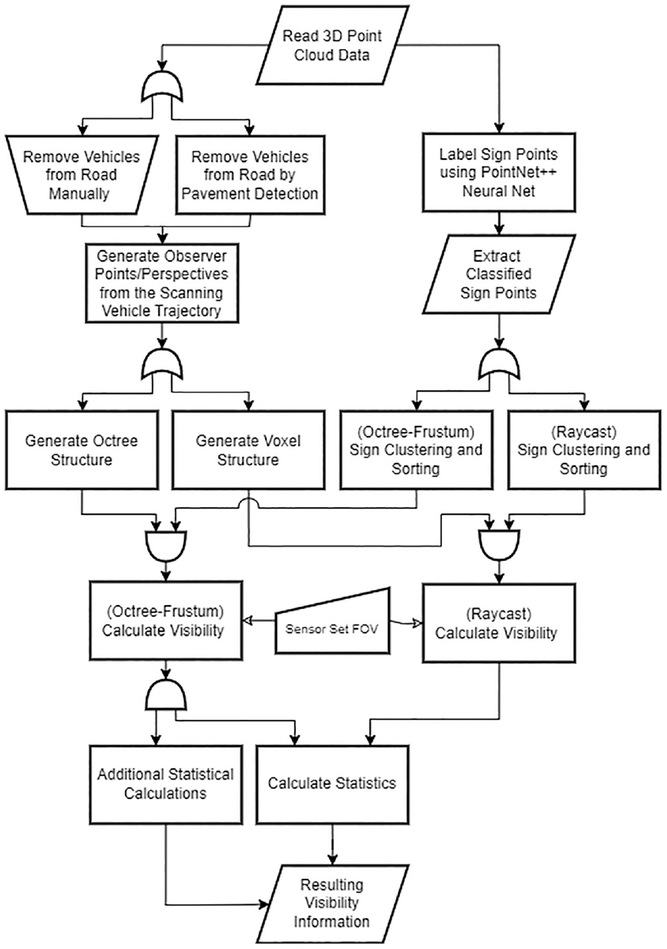
Methodology flowchart (comparing both methods).

Preprocessing

Before using the proposed method, the input point cloud ( $L$ ) must have all sign points labeled. The method described in Gouda et al. ( 13 ) was used to segment the point cloud data into sign, pavement, and non-sign-pavement points. Details on segmentation details are not given in this paper; there are several other methods to perform this task. In our previous work ( 13 ), we tackled several challenges arising in previous methods. These include the variation in point cloud density, low performance for large metric scale scenes, and a loss of geometric information about the point clouds in down-sampling. The next preprocessing step was to remove vehicles on the road. Vehicles were found by searching above the pavement for point clusters. Objects up to 2 m above the pavement, identified as vehicles, were excluded from the input point cloud $L$ . It is important to note that this study focuses on physical infrastructure occlusions; dynamic occlusions caused by other road users are not considered. A manual review was conducted to ensure that the removed points belonged to vehicles.

Defining Observers

In this work, an observer is defined as a set of points following a vehicle’s trajectory that simulates the visibility positions for an AV. First, the car’s trajectory was extracted from lidar data by taking points with zero scan angle and sorting them by GPS time. All selected points were then smoothed using a window to create a curve describing the car’s trajectory. Along the curve, points were sampled every 1 m and shifted up by 1.2 m, leading to a set of observers ( $O$ ).

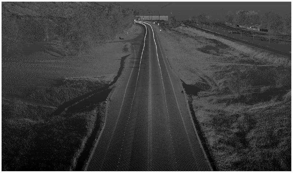
To explore the full potential of a point cloud, a second set of observers ( $O_{opp}$ ) was defined to consider a car driving in the opposite direction to the first set. This was done by simply shifting each observer in the original observer set, $O$ , 4 m to its left and flipping its orientations and order. This works on standard, non-separated, two-way, two-lane highways because of the simple geometry of the road surface. In other cases, a manual method was used by selecting control points in the opposite lane. Observer points were then generated by interpolating them 1 m apart between the control points and translating them upwards by 1.2 m (Figure 2).

Figure 2.

Observer points in both directions along a two-way two-lane road.

Data Structures

Raycast Method: Voxelated Point Cloud

The raycast method involved using a voxelated point cloud to determine obstructions and reduce processing time. The input point cloud $L$ was grouped into coordinate axis aligned cubes of 0.15 m agglomeration points. To store voxels, a 3D Adelson-Velsky–Landis tree was used. Additionally, the voxels are larger than points and more effectively block near raycasts. Without voxelating the point cloud, raycasts could sometimes fit between points that should otherwise be considered an obstruction, surface, and so forth. Therefore, voxels essentially densify the point cloud for raycast analysis while also decreasing processing time.

Octree-Frustum Method: Octrees and Half-Spaces

The convex hull method uses an octree, which is a space-portioning data structure effective in storing 3D data. Octrees, like their 2D counterpart, binary trees, enable spatial searching and queries in logarithmic time. This is done by dividing space into eight octants or cuboidal nodes and grouping points in each octant according to their position, up to a maximum number of points. Beyond this maximum, any arbitrary node is recursively subdivided into eight smaller child octants until none of the child nodes of the octree contains more than the maximum number of points per node. Queries into the octree search for points in a volume bounded by a set of constraints. Such constraints are represented by the intersection of half-spaces, given as

\begin{matrix} H = h_{1} \cap h_{2} \cap \dots \cap h_{n} \end{matrix}

(1)

A half-space is either of the two subspaces obtained when a hyperplane divides affine space. In three dimensions, this refers to the two volumes on either side of an infinite plane. A half-space is given by

\begin{matrix} h_{i} = (x, y, z) \in R^{3} | a_{i} x + b_{i} y + c_{i} z \geq d_{i} \end{matrix}

(2)

with constants $a_{i}, b_{i}, c_{i}, d_{i}$ . This is similar to the plane equation in three dimensions, which is an equality. The half-space equation is different as it defines any point on or greater than the plane to be a part of the half-space (the other half-space being less than the plane). In this case, points on the plane, that is, the boundary of the volume, will be considered a part of the volume; therefore the half-space is defined as inclusive.

The intersection of a set of half-spaces in three dimensions forms a convex polyhedron. If the volume of the intersection is finite, or bounded, the constraints may be used as an input into the octree for query or search purposes. Figure 3 shows what this may look like in three dimensions.

Figure 3.

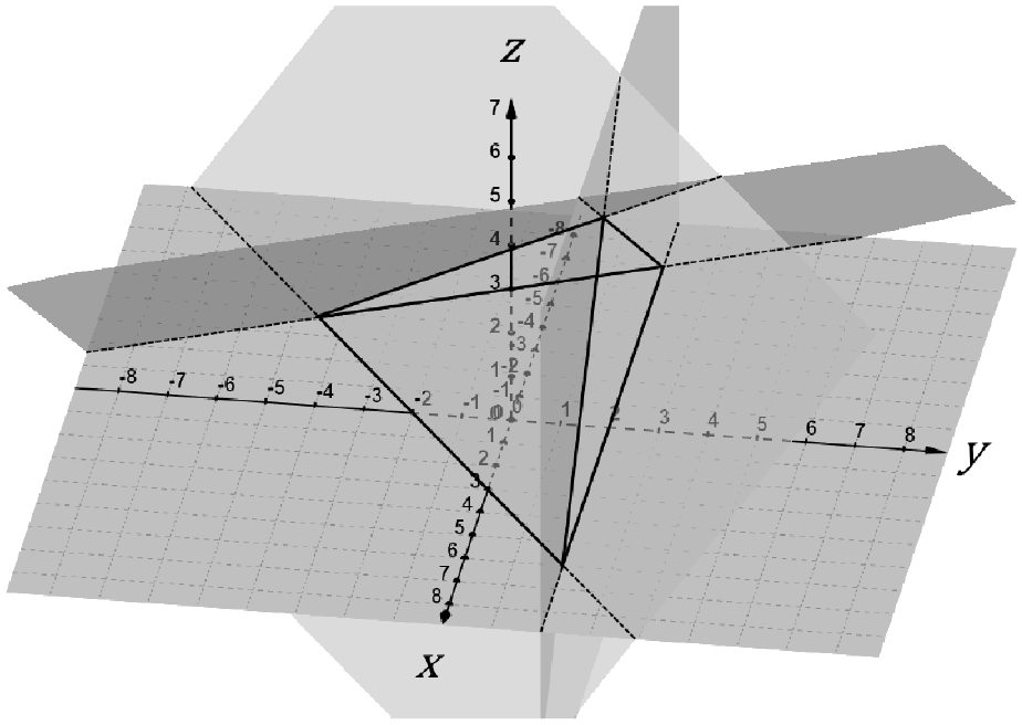
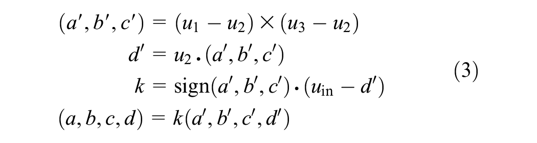
Example intersection of four half-spaces forming bounded volume: $H_{Figure 3} = (2, 3, - 2, - 6) \cap (- 2, - 1, 3, 12) \cap (0, 0, 1, 0) \cap (0, 1, 0, 2)$

The equation of a half-space can be found with three non-colinear points ( $u_{1}, u_{2}, u_{3}$ ) on the plane or boundary, and a point inside the half-space ( $u_{in}$ ) for confirmation of the correct side of the plane. This is possible as the normal to the plane corresponds to the coefficients a_i, b_i, and c_i, which can be found from the three non-colinear points on the plane that are then also used to find d_i, as

\begin{matrix} (a', b', c' \end{matrix}) = (u_{1} - u_{2}) \times (u_{3} - u_{2}) d' = u_{2} • (a', b', c') k = sign (a', b', c') • (u_{in} - d') \begin{matrix} (a, b, c, d) = k (a', b', c', d') \end{matrix}

(3)

Sign Clustering and Sorting

Raycast Method

In the raycast method, signs were clustered based strictly on proximity to each other. Points were clustered such that no two clusters were within 0.5 m of each other. After defining these separate clusters as individual signs, their mean center points were calculated. Using the center points of these sign clusters, the closest observer to the sign was calculated and used to determine the sign’s distance from the road. Signs beyond 20 m from the road were not considered, and such clusters were removed from the sign set. The remaining sign center points formed the set $C_{all}$ .

A set of signs $S \subset C_{all}$ was created by sorting signs according to a given set of observers $O$ or $O_{opp}$ to obtain an ascending sign set according to the closest observer. First, the trajectory vector ( $\vec{t}$ ) for each observer point $o_{i}$ was calculated as $\vec{t} = o_{i + 1} - o_{i}$ . Afterwards, the relative position vector ( $\vec{r}$ ) between a sign $s_{j} \in S$ and $o_{i}$ was calculated as $\vec{r} = s_{j} - o_{i}$ .

Then, the observer’s index that led to the minimum value of the dot product $\vec{t} . \vec{r}$ for a selected sign $s_{j}$ was recorded. The procedure described was repeated for all signs, leading to a relation for each sign and the index of the observer that was the closest projection of $s_{j}$ along the vehicle’s trajectory. This relation made it possible to sort $S$ according to ascending observers’ index.

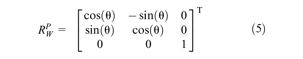
To consider observers driving in both directions for the same point cloud, $C_{all}$ was divided into two disjoint sets, $C$ and $C_{opp}$ , containing only the signs that were related to each set of observers. First, $C_{all}$ was sorted according to $O$ to give a global index for each sign. Afterwards, for the projection $p$ of each sign $c \in C_{all}$ in $O$ calculated to sort signs, the coordinates of $c$ in the coordinate system centered in $p$ and oriented following $O$ were computed.

The orientation angle $(θ)$ of the observer $o_{i} \in O$ located in $p$ was calculated by taking the vector between the next observer $o_{i + 1}$ and $o_{i}$ and calculating its angle with respect to the $xy$ plane. Therefore, for $\vec{w} = (x_{w}, y_{w}, z_{w}) = o_{i + 1} - o_{i}$ , the angle $θ$ was described as

\begin{matrix} θ = atan 2 (\frac{y_{w}}{x_{w}}) \end{matrix}

(4)

Next, the homogeneous transformation matrix ( $H_{W}^{P}$ ) from the coordinate system ( $P$ ) centered in $p$ to the global coordinate system ( $W$ ) was calculated. First, using $θ$ , the rotation matrix from $P$ to $W$ along the $z$ axis ( $R_{W}^{P}$ ) was described, as

\begin{matrix} R_{W}^{P} = {[\begin{matrix} \cos (θ) - \sin (θ) 0 \\ \sin (θ) \cos (θ) 0 \\ 001 \end{matrix}]}^{T} \end{matrix}

(5)

Defining $d_{P}^{W}$ as the vector from the origin of $W$ to the origin of $P$ , it follows that $d_{P}^{W} = p$ . The matrix $H_{W}^{P}$ can be written as a function of $R_{W}^{P}$ and $d_{P}^{W}$ :

\begin{matrix} H_{W}^{P} = [\begin{matrix} R_{W}^{P} - R_{W}^{P} \cdot d_{P}^{W} \\ 01 \end{matrix}] \end{matrix}

(6)

The matrix $H_{W}^{P}$ was calculated and applied in sign $c$ to find the coordinates of $c$ from the perspective of $p$ ( $c'$ ). If $c'$ had a negative $y$ coordinate, it was placed on the right side of $p$ and, therefore, $c \in C$ . Otherwise, $c \in C_{opp}$ . At this point, signs were separated into $C$ and $C_{opp}$ , but the order of signs in each set and their indexes were relative to the first sort. Thus, $C$ was sorted according to $O$ and $C_{opp}$ according to $O_{opp}$ , to adjust the indexes and order of the signs.

Octree-Frustum Method

In the octree-frustum method, signs were obtained by clustering points in $S_{new}$ using the DBSCAN (density-based spatial clustering of applications with noise) algorithm, such that each point in the cluster (or sign) was located at least 0.5 m away from all points in another cluster. Utilizing an orthogonal-least-squares fit (affine-fit), a plane and four corners can be assigned to these arbitrary point clusters so that they represent the sign structure and area. The orthogonal fit returns three vectors of importance, the normal vector ( $n$ ) to the sign plane and two tangential vectors ( $t_{1}, t_{2})$ corresponding to the principal directions of the shape. Also returned is the mean point ( $p_{mean}$ ) of all sign points $p \in P_{sign}$ . With this information, the corner points ( $c_{1}, c_{2}, c_{3}, c_{4}$ ) and the center of the sign ( $c_{mean}$ ) can be calculated, as

\begin{matrix} A_{\min} = min_{p \in P_{sign}} t_{1} • (p - p_{mean}) \\ A_{\max} = max_{p \in P_{sign}} t_{1} • (p - p_{mean}) \\ B_{\min} = min_{p \in P_{sign}} t_{2} • (p - p_{mean}) \\ B_{\max} = max_{p \in P_{sign}} t_{2} • (p - p_{mean}) \\ c_{1} = p_{mean} + A_{\min} t_{1} + B_{\min} t_{2} \\ c_{2} = p_{mean} + A_{\max} t_{1} + B_{\min} t_{2} \\ c_{3} = p_{mean} + A_{\max} t_{1} + B_{\max} t_{2} \\ c_{4} = p_{mean} + A_{\min} t_{1} + B_{\max} t_{2} \\ c_{mean} = \frac{1}{4} (c_{1} + c_{2} + c_{3} + c_{4}) \end{matrix}

(7)

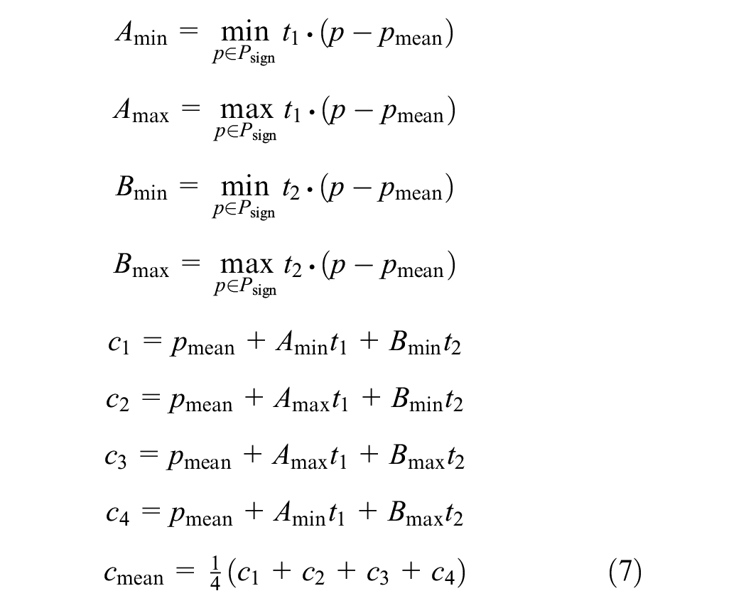
Figure 4 illustrates how this fit is applied to a point cluster.

Figure 4.

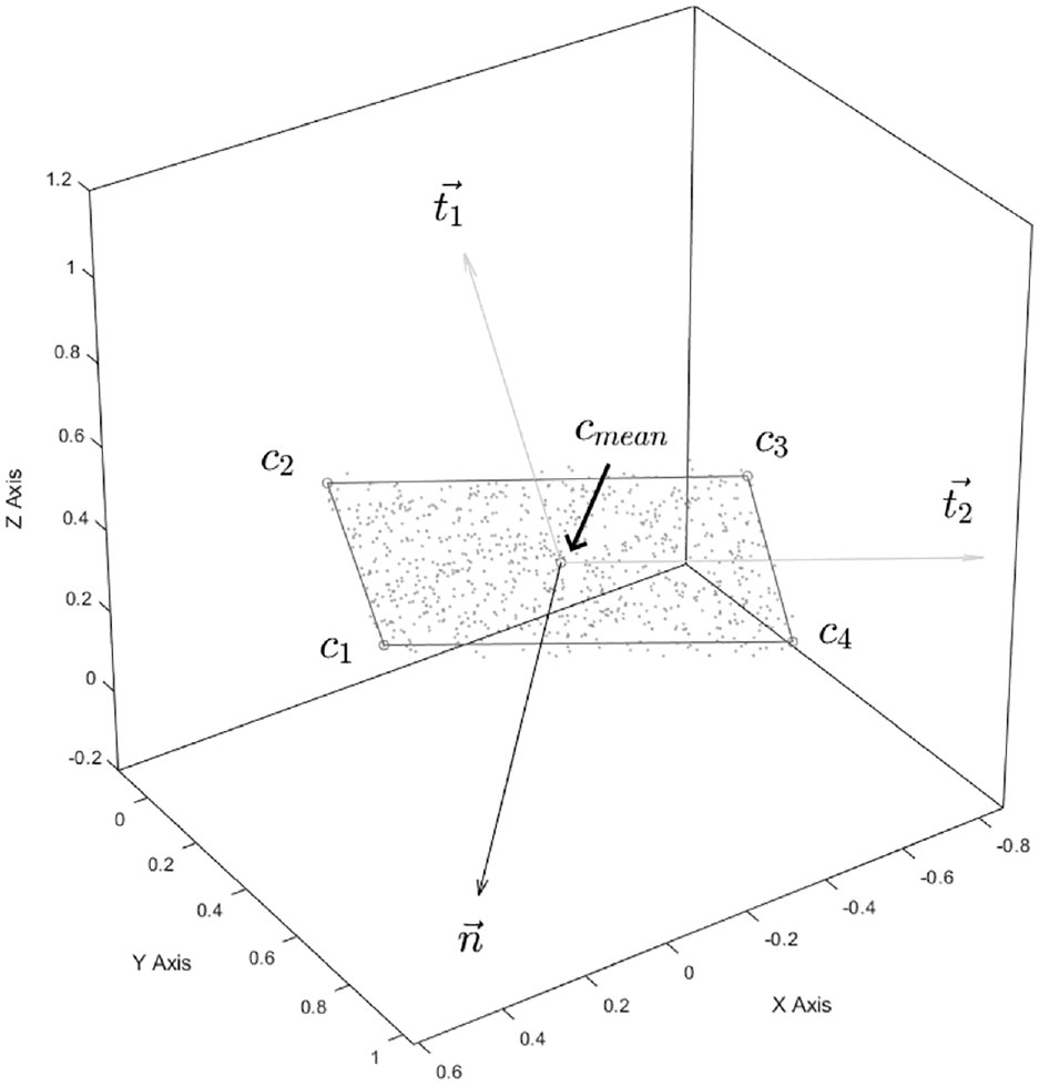
Sign point cluster fit, displaying corner points, mean point, and corresponding computed vectors.

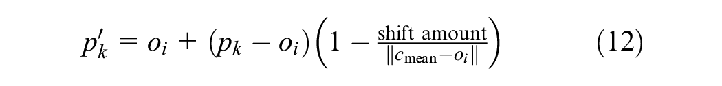
Additionally, shifted corner points can be calculated using two scaling factors ( $s_{1}, s_{2}$ ) to decrease the area of a sign. This may be useful when the details of the sign are perhaps constrained to a smaller area than the physical size of the sign, for example, when the sign has a large border. The shifted corner points ( $p_{1}, p_{2}, p_{3}, p_{4}$ ) can be calculated as

\begin{matrix} p_{1} = c_{1} + \frac{1 - s_{1}}{2} (c_{2} - c_{1}) + \frac{1 - s_{2}}{2} (c_{4} - c_{1}) \\ p_{2} = c_{2} + \frac{1 - s_{1}}{2} (c_{1} - c_{2}) + \frac{1 - s_{2}}{2} (c_{3} - c_{2}) \\ p_{3} = c_{3} + \frac{1 - s_{1}}{2} (c_{4} - c_{3}) + \frac{1 - s_{2}}{2} (c_{2} - c_{3}) \\ p_{4} = c_{4} + \frac{1 - s_{1}}{2} (c_{3} - c_{4}) + \frac{1 - s_{2}}{2} (c_{1} - c_{4}) \end{matrix}

(8)

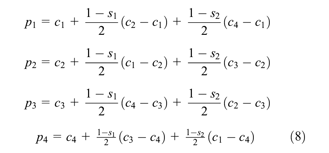
These formulas stretch the border around the sign by a ratio of $s_{1}$ in the direction of $t_{1}$ and by a ratio of $s_{2}$ in the direction of $t_{2}$ , both centered around the mean point.

The clusters were filtered so that only clusters with center points within 20 m of their closest observer were considered, to filter out distant signs from the road. The filtered center points form a set $C_{all}$ similar to the raycast method:

\begin{matrix} o_{close} = \underset{o \in O}{\arg \min} ‖ c_{mean} - o ‖ \end{matrix}

(9)

Additionally, each sign is either on the left or the right side of the road. This is determined based on the dot product of the vector from its closest observer to the sign and the leftward vector for that observer:

\begin{matrix} left \Leftrightarrow l_{close} • (c_{mean} - o) > 0 \end{matrix}

(10)

Identifying which side of the road the sign is on allows the signs to be filtered, so that one side of the road can be analyzed later by splitting $C_{all}$ into $C$ and $C_{opp}$ , corresponding to signs on the right-hand side of the corresponding observer set, $O$ or $O_{opp}$ . Lastly, the angle of the sign to the roadway can be determined. If the angle is greater than 90°, the normal is flipped to the other side of the sign, on the assumption that it would not make sense for a sign to face away from the road:

\begin{matrix} θ = acos (\frac{n • (c_{mean} - o)}{‖ c_{mean} - o ‖}) \end{matrix}

(11)

The created set of signs, $S \subset C_{all}$ , is sorted according to a given set of observers $O$ or $O_{opp}$ , to obtain an ascending sequence of signs, according to the closest observer indexes.

Defining Sensor Sets

The analysis of visibility by an AV is strongly dependent on the number of sensors and their field of view. This can vary between vehicles, which is why a simulation-based approach with configurable sensor characteristics is valuable. The number of sensors, the description of the vertical and horizontal limits, and the range for each sensor used forms a sensor set. Figure 5 shows how the individual sensor boundaries are defined.

Figure 5.

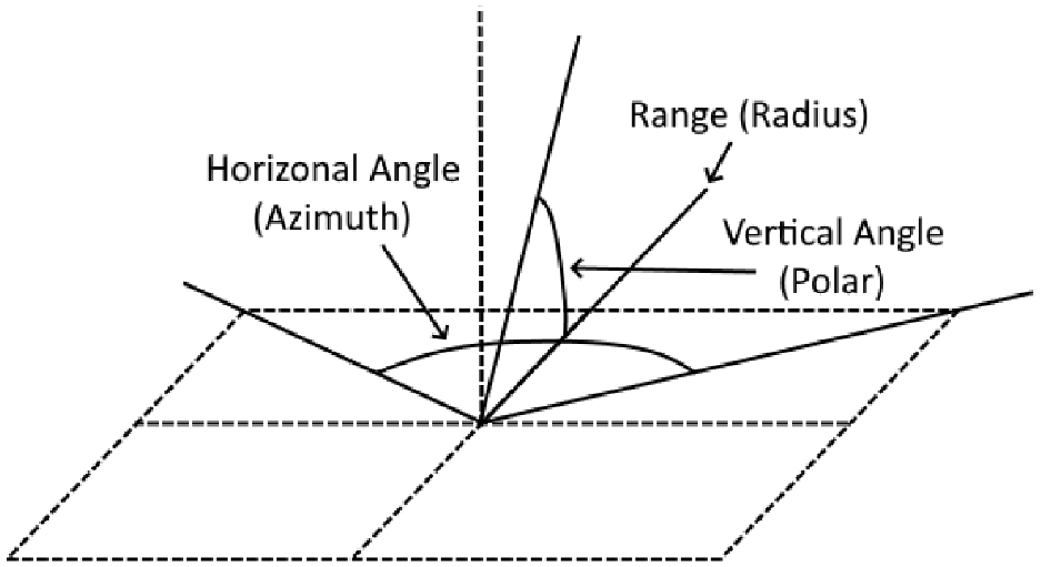
Sensor angles using spherical coordinates.

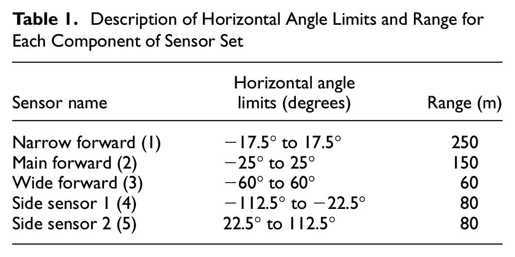
Generally, sensors are defined using spherical coordinates. This suggests that the horizontal and vertical limits or boundaries are given as azimuthal or polar angles, respectively, with the forward vector being 0° at any given observer. Therefore, each sensor has a minimum and maximum angle in each of these directions, with upwards and clockwise from the forward vector considered as the positive directions for these angles. The ranges of sensors also vary, bounding the distance of the individual sensor field of vision (FOV) arcs created by these angles and causing the FOV to appear as a section from a sphere, with the range as the radius. Figure 6 shows what this looks like for the sensors described in Table 1 ( 2 ).

Figure 6.

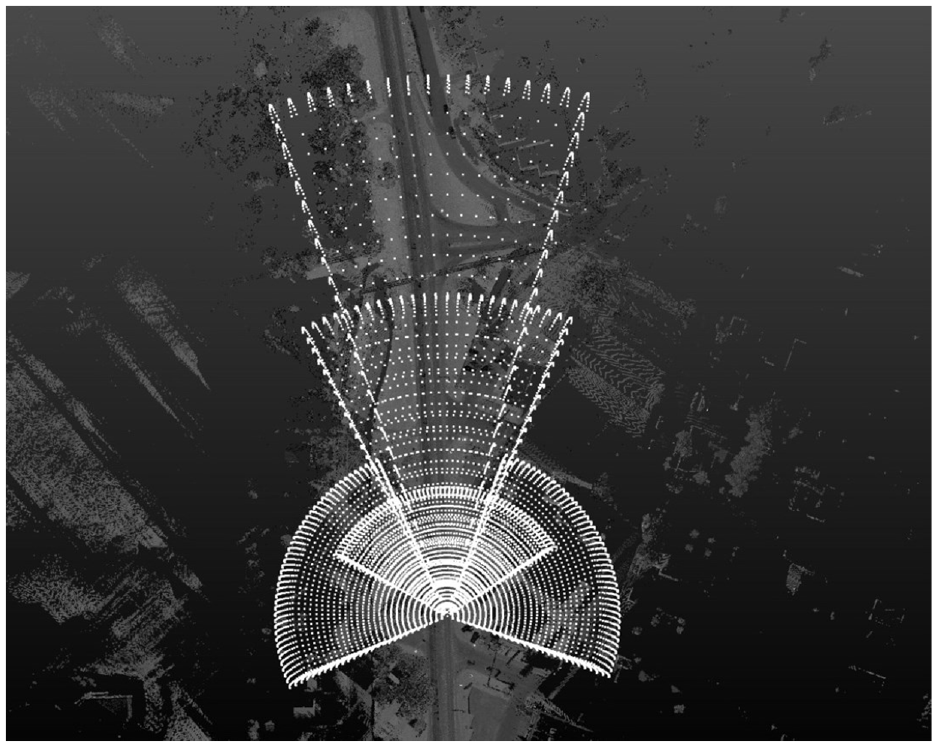
Example sensor set for the sensors described in Table 1.

Table 1.

Description of Horizontal Angle Limits and Range for Each Component of Sensor Set

Sensor name	Horizontal angle limits (degrees)	Range (m)
Narrow forward (1)	−17.5° to 17.5°	250
Main forward (2)	−25° to 25°	150
Wide forward (3)	−60° to 60°	60
Side sensor 1 (4)	−112.5° to −22.5°	80
Side sensor 2 (5)	22.5° to 112.5°	80

Calculating Visibility

Raycast Method

After data preprocessing, we can determine all observers of each set that were visible from each sign point $c_{j} \in C$ or $c_{j} \in C_{opp}$ . For every observer $o_{i} \in O$ or $o_{i} \in O_{opp}$ , all signs $c_{j} \in C$ or $c_{j} \in C_{opp}$ were considered, depending on the direction being analyzed. If the sign $c_{j}$ was not visible from $o_{i}$ , the next sign $c_{j + 1}$ was analyzed. In this AV scenario, if a sign was not visible from one observer, this means that it was not within any of the individual sensor ranges or viewing angles for the selected sensor set centered at the observer point.

For all signs within a sensor range, Bresenham’s line algorithm ( 35 ) was used to cast a ray from $o_{i}$ to $c_{j}$ and check each ordered voxel $r$ on the ray for occlusion from a voxel in $L$ . If there was an obstruction, sign $c_{j}$ was not visible from $o_{i}$ . Otherwise, $o_{i}$ was visible from $c_{j}$ . The process was repeated for each sign until the last one was analyzed for each set. For each possible direction, a matrix of visibility $(V$ or $V_{opp}$ ) was defined, in which the element of the ith line and jth column ( $v_{ij})$ was equal to 1 if the sign $j$ was visible from the observer $i$ . Otherwise, $v_{ij} = 0$ .

Octree-Frustum Method

For every observer $o_{i} \in O$ or $o_{i} \in O_{opp}$ , all signs $c_{j} \in C_{all}$ were considered. If the sign $c_{j}$ was not visible from $o_{i}$ , the next sign $c_{j + 1}$ was analyzed. Exactly as in the raycast method, if a sign was not visible from one observer, this means that it was not within range of any individual sensors or viewing angles for the selected sensor set centered at the observer point.

For all signs within a sensor range, a volume bounding frustum was created and queried against an octree organization of the point cloud $L$ to determine whether any obstructions existed between the observer $o_{i}$ and the sign $c_{j}$ . If there was an obstruction, sign $c_{j}$ was not visible from $o_{i}$ . This view frustum is a rectangular pyramid starting at the observer and ending just before the sign face, so as not to intersect the points that make up the sign itself, as this would cause errors in the evaluation of obstructions.

The apex of the view frustum is an observer, and the base of the view frustum is made up of a shifted version of the scaled corner points $p_{1}', p_{2}', p_{3}', p_{4}'$ , as discussed in the previous section and shown in Figure 7. The shift or cut-off of these points is given as

\begin{matrix} p'_{k} = o_{i} + (p_{k} - o_{i}) (1 - \frac{shift amount}{‖ c_{mean} - o_{i} ‖}) \end{matrix}

(12)

and is repeated for each scaled corner point.

Figure 7.

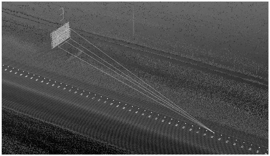
View frustum with shift of 1 m and stretch factors $s_{1} = s_{2} = 1 / \sqrt{2}$ .

To determine the intersection of half-spaces that constrain this frustum, a point inside it must be found; in turn, this would be inside all the half-spaces required to define the constraints of this volume. A point that is guaranteed to be inside this frustum is the average of the five points that make up the corners, given by

\begin{matrix} m = \frac{p'_{1} + p'_{2} + p'_{3} + p'_{4} + o_{i}}{5} \end{matrix}

(13)

Therefore, the intersection of half-spaces defining the constraints of the view frustum is given by

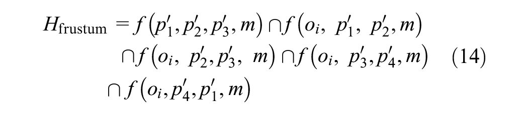
\begin{matrix} \begin{matrix} H_{frustum} = f (p'_{1}, p'_{2}, p'_{3}, m) \cap f (o_{i}, p'_{1}, p'_{2}, m) \\ \cap f (o_{i}, p'_{2}, p'_{3}, m) \cap f (o_{i}, p'_{3}, p'_{4}, m) \end{matrix} \\ \cap f (o_{i}, p'_{4}, p'_{1}, m) \end{matrix}

(14)

Then H_frustum can be passed to the octree of $L$ to query for any points that exist inside this volume. Any points that are inside the frustum obstruct the view of the observer to the sign. For each possible direction, a matrix of visibility $(V$ or $V_{opp}$ ) was defined, in which the element of the ith line and jth ( $v_{ij})$ was equal to 1 if the sign $c_{j}$ was visible from the observer $o_{i}$ , otherwise, $v_{ij} = 0$ . It should be noted that in each direction $V$ or $V_{opp}$ could be additionally segmented or filtered by $C$ or $C_{opp}$ to only the signs on the correct side of the road. However, the computation evaluates the visibility of all signs for the given observer set.

Calculating Visibility Measures

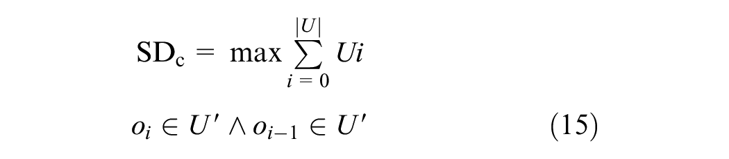
The calculated visibility score matrices were used to generate various measures, such as total visible distance and time, for each sign. If the sum of visibility scores for all observers in relation to a sign $c_{j}$ was equal to 0, then the sign was not visible from any observer $o_{i}$ . In this case, the next sign $c_{j + 1}$ was taken to be analyzed. Otherwise, the statistics for the sign were calculated.

To calculate the measures for a sign, the first visible observer $o_{f}$ and the last visible observer $o_{l}$ were used to define a set of observers, $U = {o_{f}, o_{f + 1}, \dots, o_{l - 1}, o_{l}}$ , between the first visible and last visible observer, inclusive. Then, all visible observers $U' = {o_{u} | o_{u} \in U, v_{uj} = 1}$ were found. The sets $U$ and $U'$ were used to calculate measures related to visibility. The first measure calculated was the total visible distance of the sign, given by $| U' |$ multiplied by the observer interval of 1 m. Later, the relation between $U$ and $U'$ was used to generate other information about signs. Finally, the proportion of visible observers was calculated as $| U' | / | U |$ . A comparison between the total visible time for each sign and the sensor reaction time was determined. The total visible time for a sign was defined as the total visible distance divided by design speed.

Octree-Frustum Method: Continuous Sight Distance (Alternative Sight Distance)

In the octree-frustum method, the sight distance was calculated in the same way as in the raycast method, as the sum of observers that had an unobstructed view frustum of the sign given by the visibility matrix $V$ or $V_{opp}$ . Additionally, the continuous sight distance was calculated, that is, the longest consecutive set of observers with an unobstructed view of the sign. The continuous sight distance, $S D_{c}$ , is equivalent to the longest consecutive set of indexes from $U$ that intersect $U'$ . This is described as

\begin{matrix} {SD}_{c} = max \sum_{i = 0}^{| U |} Ui \\ o_{i} \in U' \land o_{i - 1} \in U' \end{matrix}

(15)

Results and Discussion

Test Segments

The proposed method was applied to three segments of Highway 01A in Alberta, Canada. First, a segment from 12 km to 16 km along the road (Segment 1) was selected because it has a high number of signs. Two other segments were considered: one from 0 km to 4 km) along the road (Segment 2), and one from 8 km to 12 km along the road (Segment 3). Since each 4-km segment was analyzed for both possible directions, the segments generated results for 24 km. All test segments were collected in 2020 by Alberta Transportation using a REIGL VMX 450 lidar system capable of collecting 360° point cloud data. Point cloud densities ranged between 150 points/m² and 1,000 points/m², depending on the survey speed and the distance from the scanner.

Sensor Set Used

For all types of sensor analyzed, an angular resolution of 0.1° was adopted for both vertical and horizontal ranges. This work also considered vertical angles ranging from−60° .to 30° .for all sensors. The reference adopted for orientation was the $x$ axis pointed in the front of the vehicle and the $z$ axis pointing up, perpendicular to the ground.

The set was a representation of a combination of different sensors ( 2 ). Table 1 gives a description of the sensor set, and Figure 8 shows a representation of an observer field of view using the sensor set.

Figure 8.

Sensor set: each sensor field of view is represented in a different color.

Comparison of Methods

Each of the raycast and octree methods was used to analyze the sight distance to signs along a roadway segment. These methods were then compared against each other to determine inaccuracies that might have caused discrepancies in the results. This section presents and discusses several figures, comparing the different results of each method in one direction for the same 4 km segment from Highway 1A (Segment 1). Figure 9 is a comparison of sight distances on Segment 1, set $C$ , for the two methods.

Figure 9.

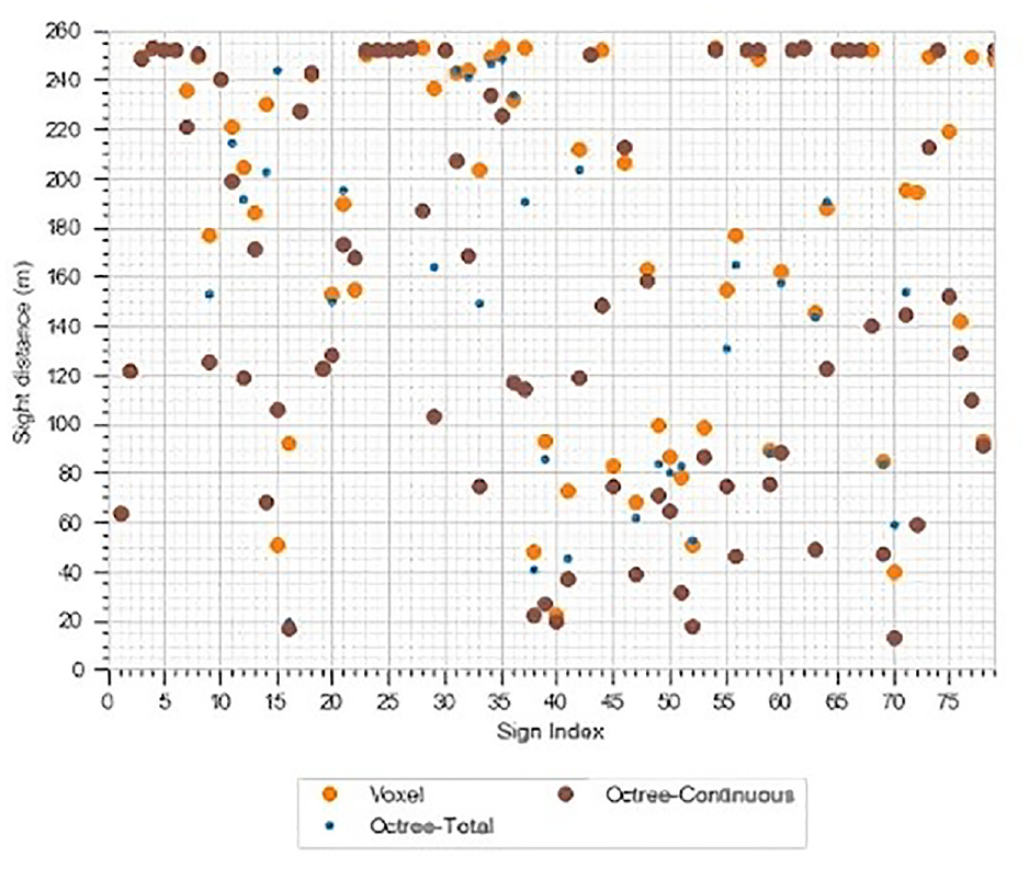
Octree versus voxel sight distance comparison for Segment 1, set C.

Three distinct types of dot can be seen in Figure 9, representing the raycast method, the octree method with continuous sight distance, and the octree method with total sight distance. The total sight distance determines for how long an observer can continuously see a traffic sign without any obstruction. Most of the discrepancies between the two octree methods are of lesser importance, as they operate differently. It is possible that the continuous sight distance to some arbitrary sign equals 1 m, while the total sight distance equals half of the maximum sensor range, 125 m, giving a difference of 124 m, in the case where consecutive observers alternate between obstructed and unobstructed. This could occur if a sign were viewed through a fence line. The discrepancies of concern are between the total sight distance of the raycast method and that of the octree method, as these results are expected to be the same.

Some of the results with large differences between the two methods were excluded. For example, Sign 33 was excluded as it was not a traffic sign and was distanced from the road, and Sign 41 was excluded as it was for a perpendicularly connecting road.

The first sign analyzed from set $C$ was Sign 21, shown in Figure 10. The octree total sight distance was calculated as 195 m, the octree continuous sight distance was calculated as 173 m, and the voxel total sight distance was calculated as 190 m.

Figure 10.

Highway 1A, Segment 1, Sign 21.

The obstructions for Sign 21 are mostly applicable to Sign 22 as well, as it is positioned approximately 75 m behind Sign 21. Additionally, Sign 21 blocks the view of Sign 22, justifying the lower sight distance calculated using both methods.

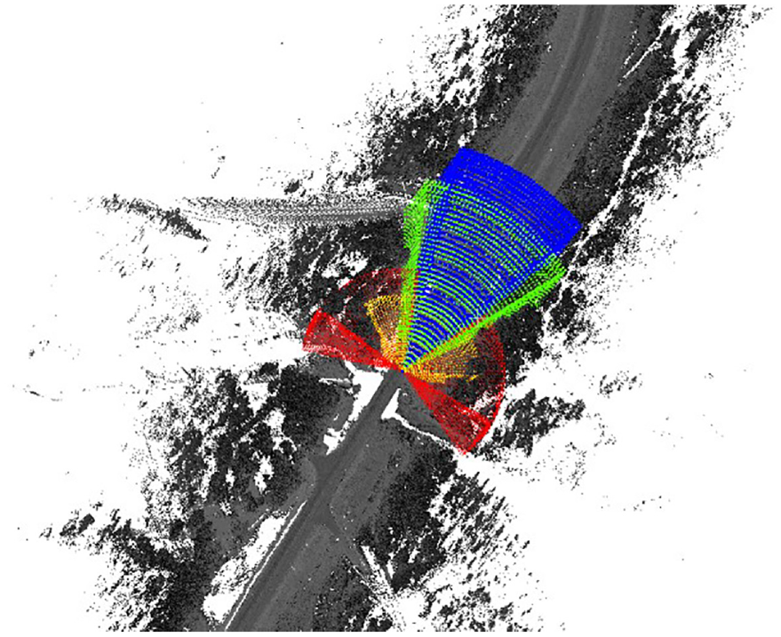
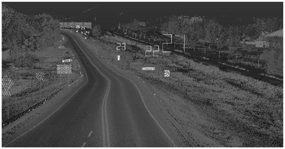
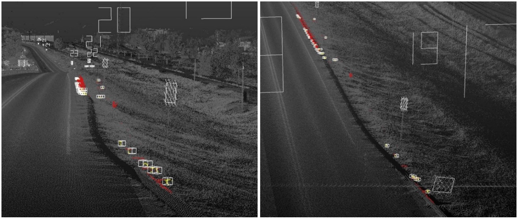
Sign 21 is blocked by several obstacles, including a guardrail, a pole, and some other points along the roadside. These points are displayed in Figure 11; Figure 12 shows a section of the raycasts, as well as a section of the octree frustums obstructed by them.

Figure 11.

Sign $c_{21} \in C$ , obstructing points.

Figure 12.

Sign $c_{21} \in C$ , raycasts and frustums from the forward- and reverse-facing perspectives.

The voxels, represented by the cubes, are those obstructing raycasts (bottom row of Figure 12); the red points are those obstructing the frustums (top row of Figure 12). Although they seem to overlap almost identically, five more raycasts are obstructed than frustums, causing a small difference in the calculated sight distances. This provides evidence of the difference in precision between the two methods.

The raycast method uses voxels and Bresenham’s line algorithm, an incremental error algorithm, to detect obstructions, based on the best approximation. When the points aggregated into a voxel group exist near one boundary of the voxel, and the raycast passes through or near an opposite boundary of that voxel, Bresenham’s line algorithm might calculate such a voxel as being in the trajectory of the raycast, when the points inside the voxel did not actually intersect the ray and were in fact a small distance away from it. This shall be referred to as clipping, because the ray clipped a voxel that contains empty space adjacent to and or near the ray.

In the octree method, clipping does not occur. The octree method bounds a specific volume independent of the point cloud itself, allowing for a precise point query into the octree against a set of equalities. By detecting possible obstructions against a set of equalities, the accuracy of the results is strictly dependent on the precision of the input point cloud.

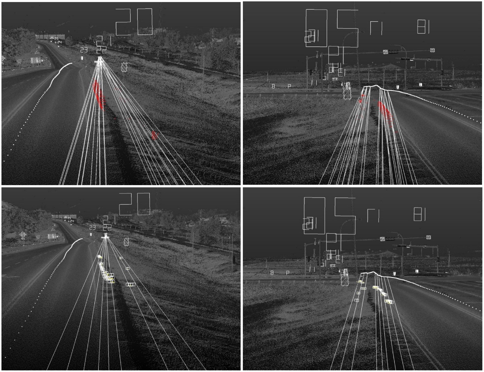
Sign 44 was also analyzed, as shown in Figure 13. Using, the raycast method, no obstruction was calculated and a maximum total sight distance of 252 m was recorded. With the octree method, the total and continuous sight distances were recorded as 150 m and 148 m, respectively. The difference in total sight distance of 102 m was caused because of Sign 43, which blocked a small portion of Sign 44. The difference between the two methods is shown in Figure 13. Figure 13a shows the raycast from potential observers to Sign 44.

Figure 13.

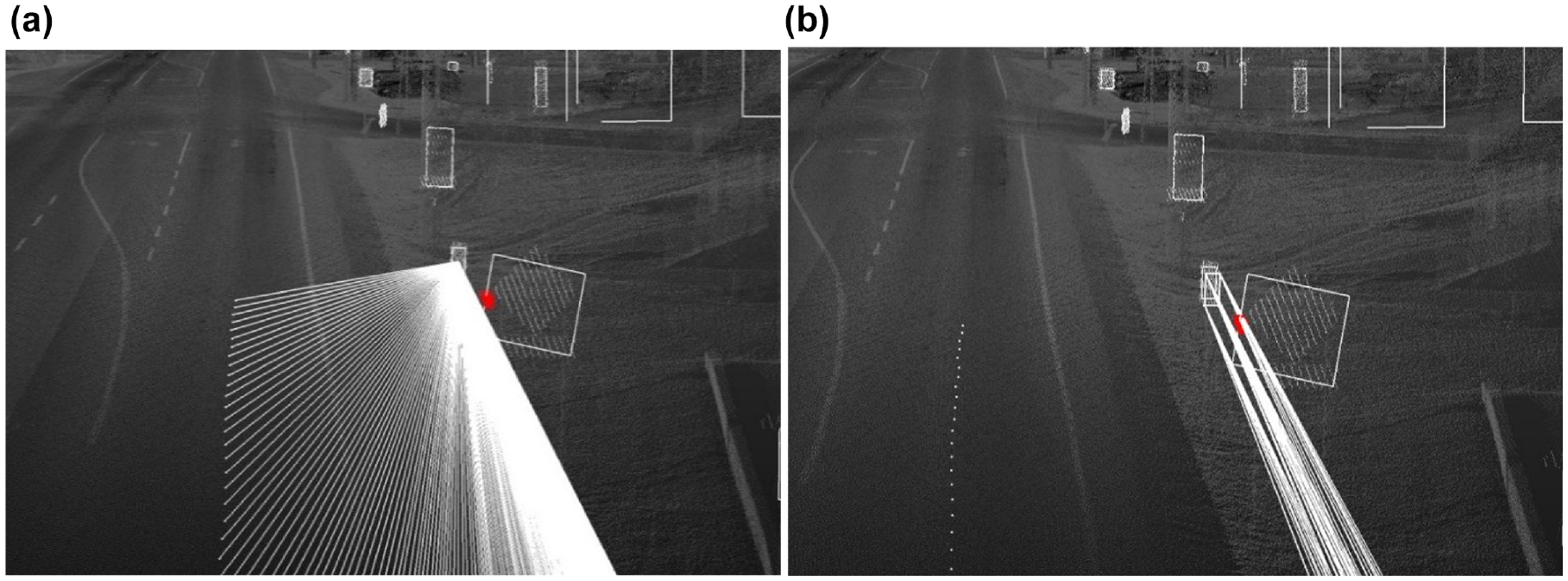
Sign $c_{44} \in C$ obstruction: (a) Raycasting method and (b) Octree method.

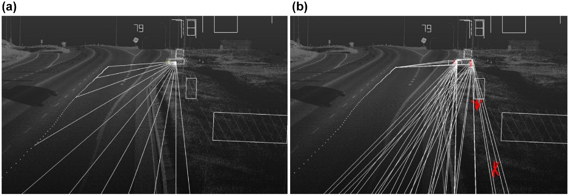
A similar problem was encountered for the last few signs of set $C$ , as shown in Figure 14. With the raycast method, only the visibility of the sign center point was evaluated, whereas for the octree method the entire sign area was considered, thus more obstructions were accurately detected.

Figure 14.

Sign $c_{77} \in C$ obstructions: (a) Raycasting method and (b) Octree method.

In many cases, the results of the two methods overlapped, with a mean percentage difference of only 1.2%, but it can be seen from the preceding examples that a large discrepancy in the results is observed in some cases, owing to the limitations of the voxel-based raycast method.

Most of the sign information needs to be visible for a certain amount of time to allow the driver to process the information and possibly take some form of action. Therefore, the octree method should be considered a more realistic representation of sign visibility as it encompasses a better majority of sign information. Because of the precision of lidar data in depicting a road environment in three dimensions, the proposed octree-based evaluation method surpasses the state-of-the-art raycast method used in previous studies in accuracy and provides a more realistic and practical result for sight distances.

Case Study for Segment 1

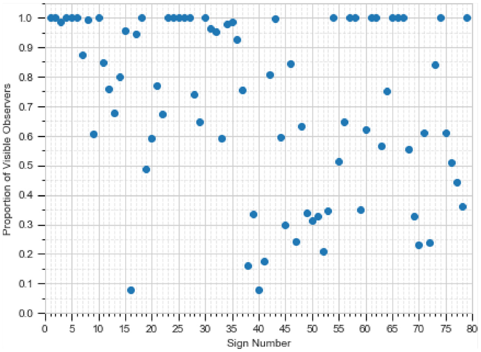
Figure 15 shows the results of the proportion of in-range observers for Highway 01A using the sensor set and analyzing the sets $O$ and $C$ . The values shown in the figure indicate that some signs have a significant number of obstruction events, compared with visible events.

Figure 15.

Proportion of visible observers for each sign number using the sensor set, considering sets $O and C .$

Using the number of visible observers, the sight distances were calculated, as shown in Figure 16. To calculate the reaction distance, the regions from Sign 1 to Sign 26 and from Sign 71 to Sign 79 were categorized as rural, while the region from Sign 27 to Sign 70 was in an urban area.

Figure 16.

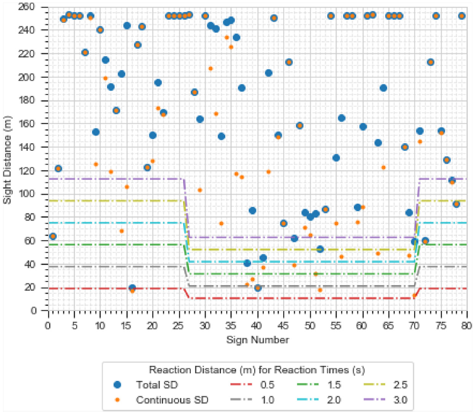
Total visible distance for each sign calculated using the sensor set.

A few signs along the segment were not visible for a sufficiently long distance to be analyzed by a road user for certain reaction times at the given speeds. Signs for which low sight distances are given in both Figures 15 and 16 would be of concern. The total visible time was computed, and the results are shown in Figure 17. Using Figures 15 to 17, a manual search was conducted for signs with poor visibility, in comparison with other signs.

Figure 17.

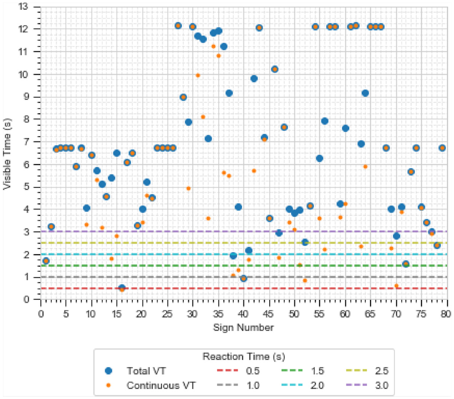
Total visible time for each sign calculated using the sensor set.

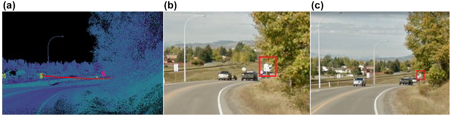
Figure 18 shows a comparison for Signs 77 and 78 along the trajectory of a vehicle. The left panel shows the point cloud for Sign 77 (green) covering parts of Sign 78 (pink) from the perspective of an observer. The middle panel of Figure 18 shows the same location, showing the same situation that was identified using the point cloud. Finally, the right panel of Figure 18 shows the same location after Sign 77 was removed and Sign 78 was replaced. This example shows the proposed methodology, in which the position of a sign replaced by Alberta Transportation is automatically extracted. Several other cases for the rest of the data are presented in Figures 19 to 22. Image data in Figures 18 to 22 were collected from Google Street View ( 36 ).

Figure 18.

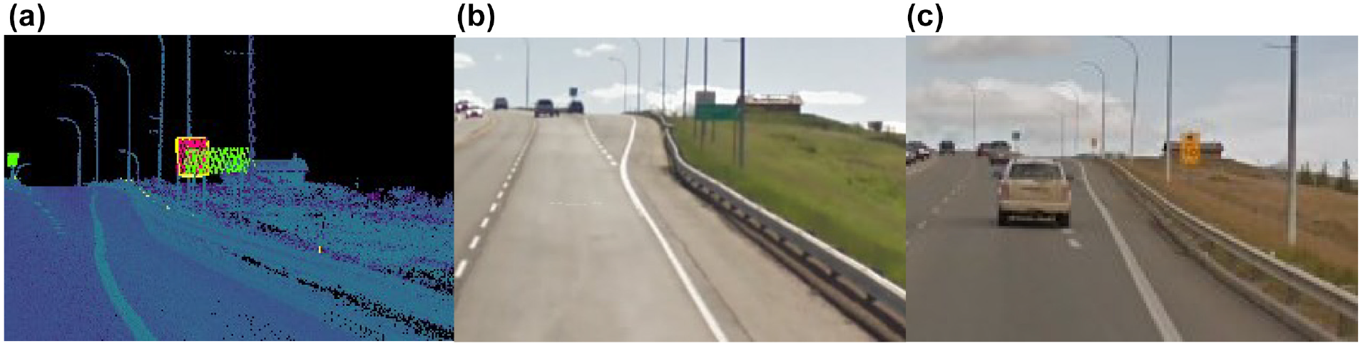
Comparison for locations of Signs 77 and 78: (a) point cloud data, (b) location before signs were changed, and (c) same location after removal of Sign 77.

Figure 19.

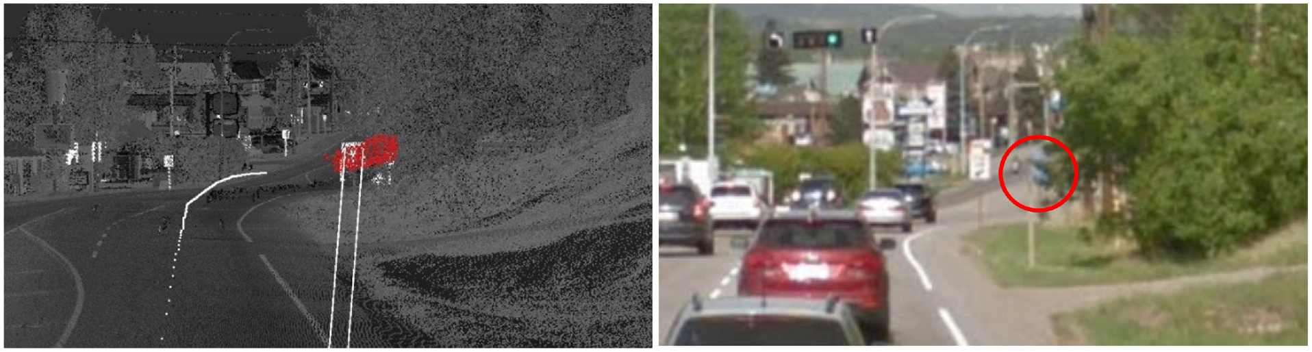
Sign obstructed by roadside tree.

Figure 20.

Comparison of locations of Signs 10, 9, and 8: (a) point cloud data, (b) location before signs were changed, and (c) same location after the change.

Figure 21.

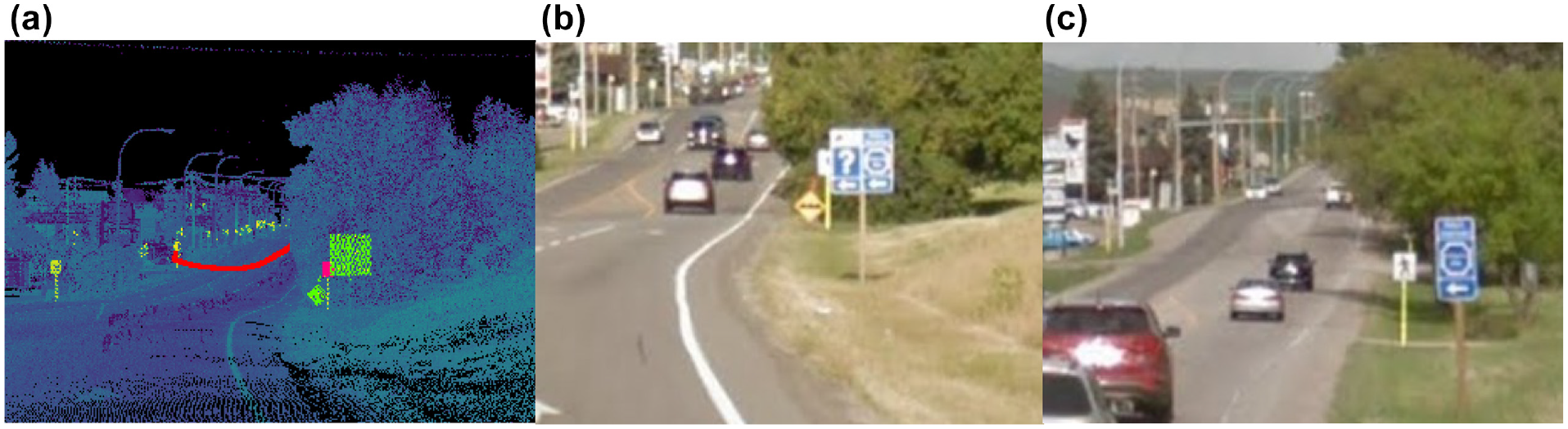
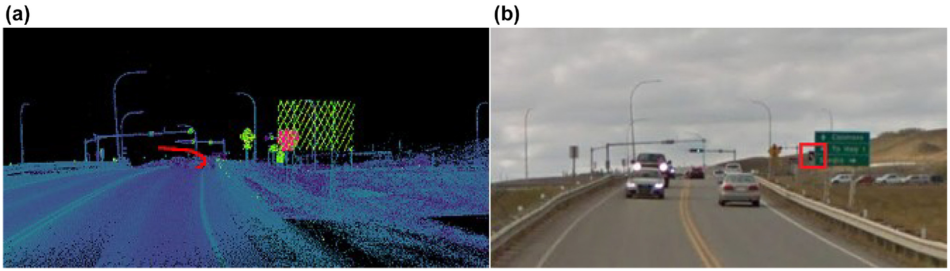
Comparison for location of Sign 31: (a) point cloud data, (b) sign after change and (c) sign before change.

Figure 22.

Sign 37 occluded by Sign 36; (a) point cloud data and (b) road.

Figure 20 (a) shows the point cloud data. In this image, Sign 10 (pink) is occluded by Sign 8. Figure 20 (b) and ( c ) show the same location before and after Sign 8 was changed to improve the sight distance.

Conclusions

The introduction of and support for AVs is becoming more widespread as manufacturers race to release high-level AVs to consumers. Despite this, government agencies have been slow to assess whether the existing road infrastructure can safely handle these vehicles. Although this is the case, research has demonstrated that AVs will rely on signs for road and safety information, in the same way as human drivers. This paper proposes a novel automated approach to assess the visibility of signs in a road environment based on AV characteristics. Although the methodology is focused on AVs, the method can be applied to human drivers. The proposed method was applied to lidar data of three different road segments in Alberta, Canada. First, semantic segmentation was used to detect traffic sign points. Visibility was assessed by sampling perspectives from the scanning vehicle’s trajectory and calculating view frustums to signs in the FOV of typical AV sensors. The input cloud was organized into an octree data structure so that the calculated view frustums were spatially queried for obstructions. The visible distance, visible time, and continuous visible distance of a sample of traffic signs were determined.

The proposed method was compared with a state-of-the-art raycasting approach, in which the input cloud is voxelated and obstructions are detected using Bresenham’s line algorithm. It was determined that the octree method is superior as it considers a 3D view perspective and the area of the sign face, whereas the raycasting approach only considers the center point of a sign and thus acts more as a point-to-point view perspective. Additionally, the octree method was found to be more precise than the raycast method. The novel methodology introduced in this study could be used to automatically identify several sign locations that had reduced visibility to AV sensors. Furthermore, three of the identified sign locations had been adjusted by Alberta Transportation since the data were collected, providing evidence of the validity of this method.

Footnotes

Acknowledgements

The authors thank Alberta Transportation for providing the data used in this study.

Author Contributions

The authors confirm contribution to the paper as follows: study conception and design: M. Gouda, K. El-Basyouny; data collection: M. Gouda; analysis and interpretation of results: M. Gouda, K. El-Basyouny; draft manuscript preparation: M. Gouda, K. El-Basyouny. All authors reviewed the results and approved the final version of the manuscript.

Declaration of Conflicting Interests

The author(s) declared no potential conflicts of interest with respect to the research, authorship, and/or publication of this article.

Funding

The author(s) disclosed receipt of the following financial support for the research, authorship, and/or publication of this article: The authors acknowledge the support of the Natural Sciences and Engineering Research Council of Canada (NSERC) and the support of Alberta Innovates and Killam Laureates. These were PhD student awards and scholarships.

ORCID iDs

Maged Gouda

Karim El-Basyouny

The contents of this paper reflect the views of the authors, who are responsible for the facts and the accuracy of the data presented. The contents do not necessarily reflect the official views or policies of Alberta Transportation.

References

Waymo. Waymo Technology. https://waymo.com/tech/. Accessed August 13, 2023.

Tesla. Tesla Future of Driving. https://www.tesla.com/en_CA/autopilot?redirect=no. Accessed September 2, 2023.

U.S. Department of Transportation. Preparing for the Future of Transportation: Automated Vehicles 4.0. 2020. https://www.transportation.gov/av/4. Accessed August 1, 2023.

Transport Canada. Transport Canada Innovative Technologies: Automated and Connected Vehicles. https://www.tc.gc.ca/en/services/road/innovative-technologies/automated-connected-vehicles.html.

SAE International. SAE: Levels of Driving Automation. https://www.sae.org/news/press-room/2018/12/sae-international-releases-updated-visual-chart-for-its-“levels-of-driving-automation”-standard-for-self-driving-vehicles.

Khoury

Amine

Highway Geometric Design Changes in Response to a Fully Autonomous Vehicle Fleet. Presented at 98th Annual Meeting of the Transportation Research Board, Washington, D.C., 2019.

Khoury

Amine

Saad

R. A.

An Initial Investigation of the Effects of a Fully Automated Vehicle Fleet on Geometric Design. Journal of Advanced Transportation, Vol. 2019, 2019. https://doi.org/10.1155/2019/6126408%0AResearch.

Gouda

Pawliuk

Mirza

El-Basyouny

Using Convex Hulls with Octree/Voxel Representations of Point Clouds to Assess Road and Roadside Geometric Design for Automated Vehicles. Automation in Construction, Vol. 154, 2023, p. 104967. https://doi.org/10.1016/j.autcon.2023.104967.

Gouda

Mirza

Weiß

Ribeiro Castro

El-Basyouny

Octree-Based Point Cloud Simulation to Assess the Readiness of Highway Infrastructure for Autonomous Vehicles. Computer-Aided Civil and Infrastructure Engineering, Vol. 36, No. 7, 2021, pp. 922–940. https://doi.org/10.1111/mice.12643.

10.

Kilani

Gouda

Weiß

El-Basyouny

Safety Assessment of Urban Intersection Sight Distance Using Mobile LiDAR Data. Sustainability (Switzerland), Vol. 13, No. 16, 2021, p. 9259. https://doi.org/10.3390/su13169259.

11.

Agina

Shalkamy

Gouda

El-Basyouny

Automated Assessment of Passing Sight Distance on Rural Highways Using Mobile LiDAR Data. Transportation Research Record: Journal of the Transportation Research Board, 2021. 2675: 676–688.

12.

Wang

Impacts on the Geometric Design of Highway from Non-Autonomous to Autonomous Vehicles (L1~L4). Presented at 98th Annual Meeting of the Transportation Research Board, Washington, D.C., 2019.

13.

Gouda

Epp

Tilroe

El-Basyouny

Traffic Sign Extraction Using Deep Hierarchical Feature Learning and Mobile Light Detection and Ranging (LiDAR) Data on Rural Highways. Journal of Intelligent Transportation Systems: Technology, Planning, and Operations, Vol. 27, No. 5, 2023, pp. 643–664. https://doi.org/10.1080/15472450.2022.2074792.

14.

Gouda

El-Basyouny

Epp

A Deep Learning Algorithm to Extract Traffic Signs from Point Cloud Data. Presented at 99th Annual Meeting of the Transportation Research Board, Washington, D.C., 2020.

15.

Zhang

Wang

Lin

Wen

Yang

Zhang

Automated Visual Recognizability Evaluation of Traffic Sign Based on 3D Lidar Point Clouds. Remote Sensing, Vol. 11, No. 12, 2019, pp. 10–14. https://doi.org/10.3390/rs11121453.

16.

Wen

Luo

Chen

Wang

Using Mobile Lidar Point Clouds for Traffic Sign Detection and Sign Visibility Estimation. Proc., 2015 IEEE International Geoscience and Remote Sensing Symposium (IGARSS), Milan, Italy, IEEE, New York, 2015, pp. 565–568. https://doi.org/10.1109/IGARSS.2015.7325826.

17.

de la Escalera

Moreno

Puente

E. A.

Salichs

M. A.

Neural Traffic Sign Recognition for Autonomous Vehicles. Proceedings of IECON’94 - 20th Annual Conference of IEEE Industrial Electronics, Bologna, Italy, IEEE, New York, 1994.

18.

Guo

Cheng

Chen

Yang

Detection of Occluded Road Signs on Autonomous Driving Vehicles. Proc., IEEE International Conference on Multimedia and Expo, Shanghai, China, IEEE, New York, 2019. https://doi.org/10.1109/ICME.2019.00152.

19.

Lawson

Roads That Cars Can Read: Report III - Tackling the Transition to Automated Vehicles. 2018. http://www.eurorap.org/new-report-tackles-the-transition-to-automated-vehicles-on-roads-that-cars-can-read/%0A; https://trid.trb.org/view/1527921.

20.

FHWA. Manual on Uniform Traffic Control Devices for Streets and Highways. Federal Highway Administration, Washington, D.C., 2009.

21.

Gouda

Shalkamy

El-Basyouny

Fully Automated Algorithm for Light Pole Detection and Mapping in Rural Highway Environment Using Mobile Light Detection and Ranging Point Clouds. Transportation Research Record: Journal of the Transportation Research Board, 2022. 2676: 617–629.

22.

Yue

Gouda

El-Basyouny

Automatic Detection and Mapping of Highway Guardrails from Mobile Lidar Point Clouds. Proc., IEEE International Geoscience and Remote Sensing Symposium (IGARSS), Brussels, Belgium, IEEE, New York, 2021. https://doi.org/10.1109/IGARSS47720.2021.9553055.

23.

Habib

Gouda

El-Basyouny

Calibrating Design Guidelines Using Mental Workload and Reliability Analysis. Transportation Research Record: Journal of the Transportation Research Board, 2020. 2674: 360–369.

24.

Gouda

Arantes de Achilles Mello

El-Basyouny

Automated Object Detection, Mapping, and Assessment of Roadside Clear Zones Using Lidar Data. Transportation Research Record: Journal of the Transportation Research Board, 2021. 2675: 432–448.

25.

Gouda

Chowdhury

Weiß

Epp

El-Basyouny

Automated Assessment of Infrastructure Preparedness for Autonomous Vehicles. Automation in Construction, Vol. 129, 2021, p. 103820. https://doi.org/10.1016/j.autcon.2021.103820.

26.

Gargoum

S. A.

El Basyouny

Shalkamy

Gouda

Feasibility of Extracting Highway Vertical Profiles from LiDAR Data. Canadian Journal of Civil Engineering, Vol. 45, 2018, pp. 418–421. https://doi.org/10.1139/cjce-2017-0620.

27.

Shladover

S. E.

Bishop

Road Transport Automation as a Public–Private Enterprise. Proc., Transportation Research Board Conference Proceedings, Washington, D.C., 2015.

28.

Wahyono

L. Kurnianggoro.

Hariyono

K.-H.

Traffic Sign Recognition System for Autonomous Vehicle Using Cascade SVM Classifier. Proc., IECON 2014 - 40th Annual Conference of the IEEE Industrial Electronics Society, Dallas, TX, IEEE, New York, 2014. https://doi.org/10.1109/IECON.2014.7049114.

29.

Walters

J. G.

Meng

Jing

Marsh

Rural Positioning Challenges for Connected and Autonomous Vehicles. Proc., ION 2019 International Technical Meeting of The Institute of Navigation, Reston, VA, 2019. https://doi.org/10.33012/2019.16727.

30.

Chen

Zhang

Mao

Design of a Multi-Sensor Cooperation Travel Environment Perception System for Autonomous Vehicle. Sensors (Switzerland), Vol. 12, No. 9, 2012, pp. 12386–12404. https://doi.org/10.3390/s120912386.

31.

Geese

Seger

Paolillo

Detection Probabilities: Performance Prediction for Sensors of Autonomous Vehicles. Proc., IS and T International Symposium on Electronic Imaging Science and Technology, Vol. 30, 2018, pp. 148-1–148-1. https://doi.org/10.2352/ISSN.2470-1173.2018.17.AVM-148.

32.

Wali

S. B.

Abdullah

M. A.

Hannan

M. A.

Hussain

Samad

S. A.

Ker

P. J.

Mansor

M. B.

Vision-Based Traffic Sign Detection and Recognition Systems: Current Trends and Challenges. Sensors (Switzerland), Vol. 19, No. 9. 2019, p. 2093. https://doi.org/10.3390/s19092093.

33.

Hirt

P. R.

Holtkamp

Hoegner

Stilla

Occlusion Detection of Traffic Signs by Voxel-Based Ray Tracing Using Highly Detailed Models and MLS Point Clouds of Vegetation. International Journal of Applied Earth Observation and Geoinformation, Vol. 114. 2022, p. 103017. https://doi.org/10.1016/j.jag.2022.103017.

34.

Huang

Cheng

Chen

Luo

Wang

Traffic Sign Occlusion Detection Using Mobile Laser Scanning Point Clouds. IEEE Transactions on Intelligent Transportation Systems, Vol. 18, No. 9, 2017, pp. 2364–2376. https://doi.org/10.1109/TITS.2016.2639582.

35.

Bresenham

J. E.

Algorithm for Computer Control of a Digital Plotter. IBM Systems Journal, Vol. 4, No. 1, 1965, pp. 25–30.

36.

Google Maps. Explore Street View and Add Your Own 360 Images to Google Maps. https://www.google.com/streetview/. Accessed April 15, 2024.

Evaluation of Traffic Sign Occlusion for Autonomous Vehicles Using Point Cloud Data

Abstract

Keywords

Literature Review

Methodology

Preprocessing

Defining Observers

Data Structures

Raycast Method: Voxelated Point Cloud

Octree-Frustum Method: Octrees and Half-Spaces

Sign Clustering and Sorting

Raycast Method

Octree-Frustum Method

Defining Sensor Sets

Calculating Visibility

Raycast Method

Octree-Frustum Method

Calculating Visibility Measures

Octree-Frustum Method: Continuous Sight Distance (Alternative Sight Distance)

Results and Discussion

Test Segments

Sensor Set Used

Comparison of Methods

Case Study for Segment 1

Conclusions

Footnotes

Acknowledgements

Author Contributions

Declaration of Conflicting Interests

Funding

ORCID iDs

References