
Abstract
The goal of Vision Zero is the prevention of all traffic fatalities and serious injuries. Although traditional transportation planning is reactive to locations where serious crashes occur, some agencies are taking a more proactive approach to safety to improve locations with high expected crashes before someone is seriously injured or killed. This paper presents the results of a systemic safety analysis that produced two pedestrian-related safety performance functions for Montgomery County, MD, including 1) motor vehicle crashes with pedestrians at intersections at night and 2) through-movement motor vehicle crashes with pedestrians at road sections. These models were built using negative binomial regression of police-reported crash data collected from 2015 to 2019 for most of the county road network integrated with land use-, demographic-, and roadway variables collected by the Montgomery County Planning Department for 16,387 intersections (stop-controlled and signalized) and 29,715 segments (all functional classifications except freeways). Both models identified key transportation-related exposure variables, including motor vehicle and pedestrian volumes, proximity to transit, and crosswalk locations; they also presented land use contexts that may explain where pedestrians are likely to walk and be exposed to crash risks. These results build on current systemic safety literature and demonstrate the data collection and analysis methods that can be used in a county-level Vision Zero context to improve safety for all who walk. This paper summarizes the analysis approach, including exposure modeling, crash modeling, and applications for identifying both high-risk locations and potential mitigations. Considerations for equity and long-term planning are also discussed.
Pedestrian fatalities in the United States have reached a four-decade high. In 2021, approximately 7,485 pedestrians were killed on U.S. roads, an 11.5% increase in the number of pedestrian fatalities from 2020 ( 1 ). State trends have typically followed similar trajectories, with rising pedestrian mortality over the last several years, or have remained relatively stagnant with disproportionately high pedestrian crash involvement. In Maryland, for example, 126 pedestrians were killed in 2021, compared with 131 in 2020 and 125 in 2019 ( 1 ). Pedestrian fatalities in Maryland in these years accounted for over 20% of all traffic fatalities in the state ( 2 ).
To address this worrying trend, safety professionals are embracing more proactive, preventive approaches to road safety management. The systemic safety approach is intended to be a proactive process wherein risks are identified throughout a network and treated before crashes occur. Safety performance functions (SPFs) for systemic approaches have been developed for the city of Seattle ( 3 , 4 ), and other systemic risk analyses have been developed for the states of Oregon ( 5 ), Arizona ( 6 ), and for major arterial corridors in California ( 7 ). These systemic tools represent major contributions to determining locations of potential risk to pedestrians and can aid practitioners in identifying suitable locations for systemic treatments at midblock locations along segments ( 3 , 4 ), along segments at night ( 3 , 4 ), at intersections along major roads, and across entire roadway networks ( 5 – 7 ). However, the statewide tools lack local contextualization, and more analyses are needed to build on the Seattle SPFs, especially to specify the local land use-, equity-, and exposure contexts, as these may enable practitioners to better predict and understand risks to pedestrian safety for the study area.
Agencies seeking to realize a Vision Zero goal, meaning zero deaths or serious injuries on their roadways, often prioritize reducing pedestrian crashes resulting from pedestrians’ relatively high susceptibility to injury and the relatively low cost of pedestrian treatments. As part of its Vision Zero efforts, the Montgomery County Planning Department (MCPD) collaborated with researchers to develop a set of SPFs to identify systemic safety risks. These SPFs are based on both traditional roadway safety parameters (i.e., roadway features, operational characteristics, and crash history) and contextual data (e.g., demographics, equity variables, and development types) to better identify locations of particular risk throughout the county.
This paper summarizes the SPF development efforts for two types of pedestrian-related crashes: collisions between motor vehicles and pedestrians at intersections at night, and through-movement motor vehicle crashes with pedestrians along segments. These two crash types are only two of six SPFs developed as part of the MCPD Vision Zero Predictive Safety Analysis project ( 8 ). This paper focuses on these two crash types specifically because they comprise 51% of pedestrian crashes and 54% of pedestrian severe injuries and fatalities in Montgomery County. The pedestrian-involved crash SPFs can be used in isolation to identify risks to pedestrians or used in combination with the motorist-involved and bicyclist-involved crash SPFs to screen and prioritize higher-risk sites for all road users. The analysis builds on existing systemic safety literature by developing a countywide analysis and emphasizes the importance of examining both land use and traffic volumes as measures of exposure to understand where risks to pedestrians might exist in the built environment. Subsequent sections discuss some systemic pedestrian safety literature, describe the data collection and analysis process, present the two SPFs, and conclude with sample applications of how a local government can use the results of a systemic safety analysis to support a Vision Zero program countywide.
Literature Review and Project Background
Systemic Safety in the Literature
The key difference between the systemic safety approach and a more traditional safety analysis approach is the identification of risk factors that may exist within a transportation network regardless of crash history; by using a systemic approach, practitioners may identify locations where crash risk is high, even if these locations have been missed in a hot spot analysis ( 9 ). Implementing countermeasures at these sites allows practitioners to take a proactive approach to crash prevention rather than chasing crash hot spots throughout a roadway network. The systemic safety process, as described by Preston et al., consists of six steps and is intended to move practitioners through a process of risk identification to countermeasure selection and implementation ( 10 ). Thomas et al., in the development of a systemic safety analysis method for pedestrians, refined the procedure into a seven-step process by adding an evaluation step ( 3 ).
Pedestrian crashes are ideal for systemic safety analyses for two reasons. First, pedestrian crashes, despite their overrepresentation in fatality statistics, are relatively rare, meaning that locations of risk can be missed in traditional hot spot analyses ( 4 ). Second, locations that present safety risks to pedestrians are relatively consistent and often characterized by wide streets, speed limits above 30 mph ( 11 ), and poor visibility of pedestrians ( 12 ).
To identify locations of systemic risk, researchers and departments of transportation have developed multiple systemic pedestrian safety models. Thomas et al. developed two pedestrian crash SPFs for the city of Seattle: collisions between motor vehicles and pedestrians on segments at night, and collisions between motor vehicles going straight and pedestrians on segments ( 3 ). Common risk factors identified in the two models include transit stops, lighting, number of lanes (for the crashes involving vehicles going straight), two-way left-turn lanes, speed limits (for dark crashes), crosswalks, striped parking (for thru crashes), adjacent right-turn lanes (for thru crashes), and various exposure (i.e., pedestrian and motor vehicle volume) and surrogate (e.g., population income and urban village designation) measures.
Foster et al. compiled statewide pedestrian and bicyclist crash data in Oregon. They then developed crash trees to identify target crashes for pedestrians and bicyclists, electing to focus on total crashes in urban areas for both roadway user types. Foster et al. then collected land use, demographic, and count data from urban areas within the state. The authors selected risk factors for systemic analysis from NCHRP Report 893, including roadway type, number of lanes, access density, sidewalk presence (for pedestrians), bike lane presence (for bicyclists), and speed limit, as well as contextual and demographic variables. Then they identified potential treatment sites based on equivalent property-damage-only scores used as weighting factors to identify segments where countermeasures could be implemented systemically ( 5 ).
Gooch et al. performed a systemic safety analysis of midblock pedestrian crashes in Massachusetts using a binary logistic regression modeling approach. The authors selected facilities for analysis based on roadway functional classification and crash severity. The identified risk factors for principal and minor arterials included number of travel lanes, segment length, transit stops, and various exposure and contextual variables (e.g., motor vehicle traffic and proportion of nonmotorist commuters per square mile). Segment length and transit stops were also risk factors associated with major collectors ( 13 ).
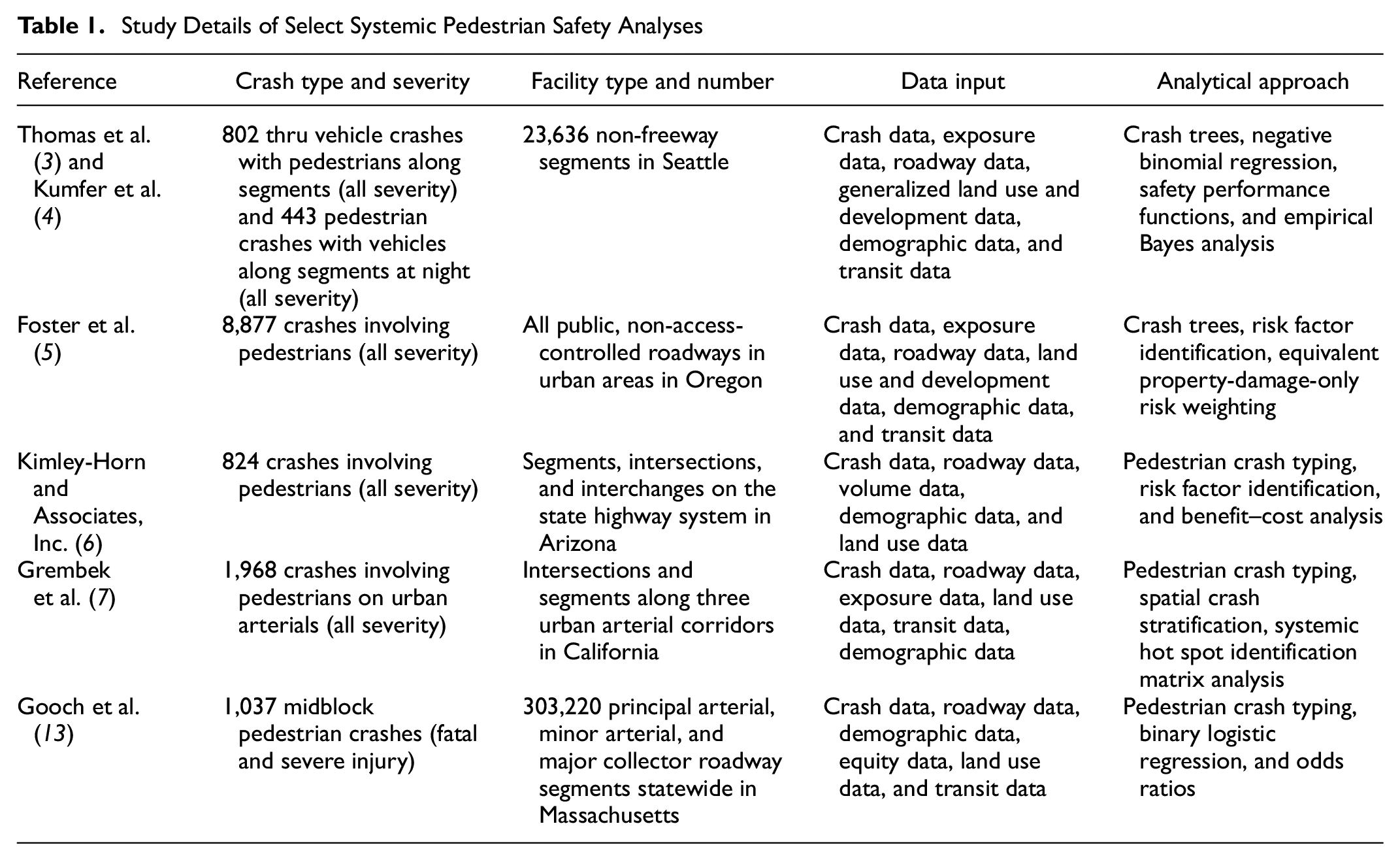
Relevant details of the systemic pedestrian safety analyses discussed in this section and the introduction are summarized in Table 1. Throughout this table, exposure data generally refer to traffic volumes for various road users; for example, the models discussed in Thomas et al. ( 3 ) and Kumfer et al. ( 4 ) use both measures of pedestrian volume and motor vehicle volume.
Study Details of Select Systemic Pedestrian Safety Analyses
Vision Zero in Montgomery County
Montgomery County, located just north of the District of Columbia, is Maryland’s most populous jurisdiction with 1.06 million residents per the 2020 Census ( 14 ). The county spans urban, suburban, and rural land contexts, including bustling urban centers, residential communities comprised of single-family homes, and a 145-mi 2 agricultural reserve primarily comprised of farmland. Although there are incorporated jurisdictions within Montgomery County, many of the county’s largest urban areas—such as Bethesda and Silver Spring—are unincorporated. As a result, 85% of the county lives in unincorporated Montgomery County, and county agencies oversee transportation planning and implementation for much of this.
Montgomery County adopted a Vision Zero Resolution in 2016 and launched its first 2-year action plan the following year. In that 2-year plan, the County set a goal of eliminating all traffic deaths by 2030. The County undertook a variety of activities to address pedestrian safety, including retiming traffic signals, issuing citations to motorists violating pedestrian safety laws, and conducting education campaigns in high-crash locations. However, the 2-year plan ( 15 ) and subsequent action plans ( 16 ) have continued to identify pedestrian safety issues as a top priority for Vision Zero activities. In fact, between 2015 and 2019, a pedestrian was struck in Montgomery County once every 18 h and killed approximately once every 31 days ( 16 ).
On reviewing crash statistics from this period, including those involving pedestrians, MCPD staff recognized that the process used in the county to identify locations of risk that could be treated was largely reactive ( 8 ) and not aligned with the more proactive methods suggested by the County’s Vision Zero commitment ( 16 ). Therefore, county staff initiated a project to develop proactive screening tools to identify locations where road users are at greatest risk, even if crashes have not yet occurred at those sites. This predictive safety analysis project is discussed more thoroughly in MCPD ( 8 ); this paper highlights the pedestrian safety components of that project, given the significant proportion of fatalities and serious injuries in crashes involving pedestrians.
Data and Methods
Analytical Approach
The methods presented in this paper build on the recent completion of NCHRP Report 893: Systemic Pedestrian Safety Analysis ( 3 , 4 ) and the NCHRP-funded implementation project for Report 893, NCHRP 20-44(13) ( 5 ). As such, the analytical method presented here generally replicates those discussed by Thomas et al. ( 3 ) and Foster et al. ( 5 ), with slight differences in the types of data collected and the countermeasure selection process. Figure 1 below shows the six-step process followed in this project.
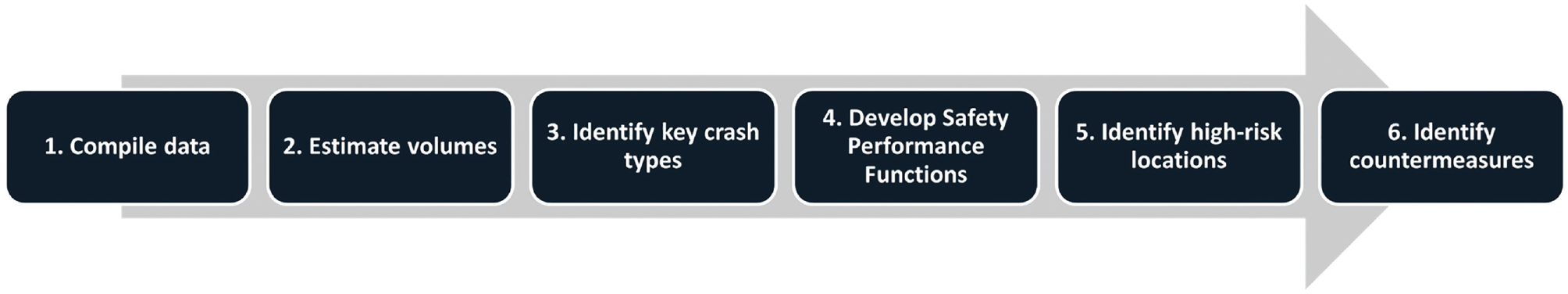
Six-step process used in the Montgomery County predictive safety analysis project.
To develop the two pedestrian SPFs, two datasets—one for intersections and one for segments—including crash, transportation facility, land use, and demographic factors were first compiled. Then, volume estimation models were developed using those datasets to produce exposure estimates that could be used in crash prediction models. To select the specific pedestrian crash types for analysis, crash trees were then developed to compare the relative frequencies of different crash types so that the most appropriate crash types could be selected. Emphasis was placed on crash frequency across the network and proportionate severity among those crashes. Then, the exposure estimates and compiled datasets were modeled to develop SPFs for the selected crash types. Systemic screening tools were then developed to identify locations in the county where risk factors relevant to the target crash types were present so that appropriate countermeasures could be selected. Although the content of this paper focuses largely on the first four steps, the SPFs developed in Step 4 were an integral part of MCPD’s systemic safety tool developed at the conclusion of this project and documented in Predictive Safety Analysis Final Report ( 8 ).
Data Sources
Two databases were created, one for segments (the length of roadway between two intersections) and another for intersections. These segments and intersections were distributed across functional classifications (from local roads to major arterials) and area types (including country areas, suburban areas, industrial areas, and urban core areas called downtowns and town centers). A variety of data were compiled and appended to the databases, including crash data, transportation data encompassing design elements within the right of way, contextual land use data, and demographic data, as well as existing multimodal counts. Generally speaking, both datasets included the same variables for land use data and demographic data, but facility-specific variables (such as number of legs for intersections or dead-end indicators for segments) were derived as appropriate. As crashes were geolocated to segments and intersections using a junction variable and a 100-ft intersection influence area buffer (for determining which crashes occurred at intersections), the appropriate values for the demographic and land use variables were assigned to those geolocations. The multimodal volume estimates were produced for segments and then assigned to adjoining intersections as discussed later in this section.
Crash Data
The analysis period included crash data from 2015 to 2019. Two pedestrian crash types were selected in cooperation with MCPD staff, with the goal of covering many crashes, severe injuries, and fatalities but to also be specific enough to point to systemic safety treatments: collisions between motor vehicles and pedestrians at intersections at night, and collisions between motor vehicles going straight and pedestrians on segments. During the study period, there were 496 pedestrian crashes after dark at intersections, 86 (17%) of which were fatal or severe. There were 418 pedestrian crashes on roadway segments with vehicles going straight, and 103 (25%) were fatal or severe. Together, these crash types comprised 51% of pedestrian crashes and 54% of total pedestrian severe injuries and fatalities between 2015 and 2019. Of note, 49% of the pedestrian dark crashes and 40% of the segment crashes occurred in the County’s Equity Emphasis Areas (EEAs). The selection of these two crash types enabled the analysis to focus on specific risks to pedestrians at intersections while capturing a range of risks to pedestrians on segments.
Transportation Data
Transportation data account for street characteristics, such as speed limit, number of lanes, roadway slope, presence and type of crosswalk, presence and type of bicycle facility, roadway classification, presence of signals and stop signs, lighting, and transit service. Although the included transportation data is expansive, it is not comprehensive. Some characteristics of the transportation network—such as indicators for bike boxes, rectangular rapid flashing beacons (RRFBs), and other specific types of pedestrian or bicycle infrastructure—were not included either because the data were not available countywide or because the transportation characteristic occurs very infrequently (e.g., there were only dozens of RRFBs spread across thousands of segments) and was therefore not expected to affect the SPFs.
During the analysis period, several capital improvements were completed throughout the county, changing the transportation attributes of individual intersections and segments. These transportation projects added a time element to the context database, including a “before” and “after” condition for some locations where conditions changed during the study period. These distinct periods were accounted for in the crash estimation models per segment and intersection.
Land Use Data
The databases also included land use variables. These variables captured the density of different land use types within different distances from the intersection or segment (within one-tenth, -quarter, and half-mile buffers). Examples of included data are parks, hospitals, gas stations, parking lots, schools, government facilities, shopping centers, alcohol-serving locations, population density, and employment density.
Demographic Data
The context data included demographic information related to income, race and ethnicity, and an aggregate EEA variable. EEAs, developed by the Metropolitan Washington Council of Governments, are a composite measure for Census tracts in the region with high concentrations of lower-income households and people of color ( 17 ).
Multimodal Counts
To understand existing travel behavior throughout the county, the context data included recent short-term multimodal counts (including motor vehicle, pedestrian, and bicycle volumes), from which estimated annual average daily volumes were developed using temporal adjustment factors.
Significant Variables
The databases developed to evaluate the two pedestrian crash types consisted of 170 segment variables and 282 intersection variables. Many of these variables were derived forms of a single measure approximated using GIS at different distances; for example, a variable for the number of metro stations within range of an intersection was calculated at the tenth of a mile, quarter of a mile, and half of a mile distance buffer. Several variables were derived to see whether different variable formats provided a better model fit, and for some variables (e.g., speed limit) both numeric and categorical versions were tested. Owing to the number of variables compiled, a table listing all variables was beyond the scope of this paper. Instead, Table 2 lists numeric and categorical variables that were used to develop annual average daily pedestrian (AADP) and annual average daily traffic (AADT) estimates, whereas Table 3 lists significant variables used in the SPF development.
Variables Used in Volume Models
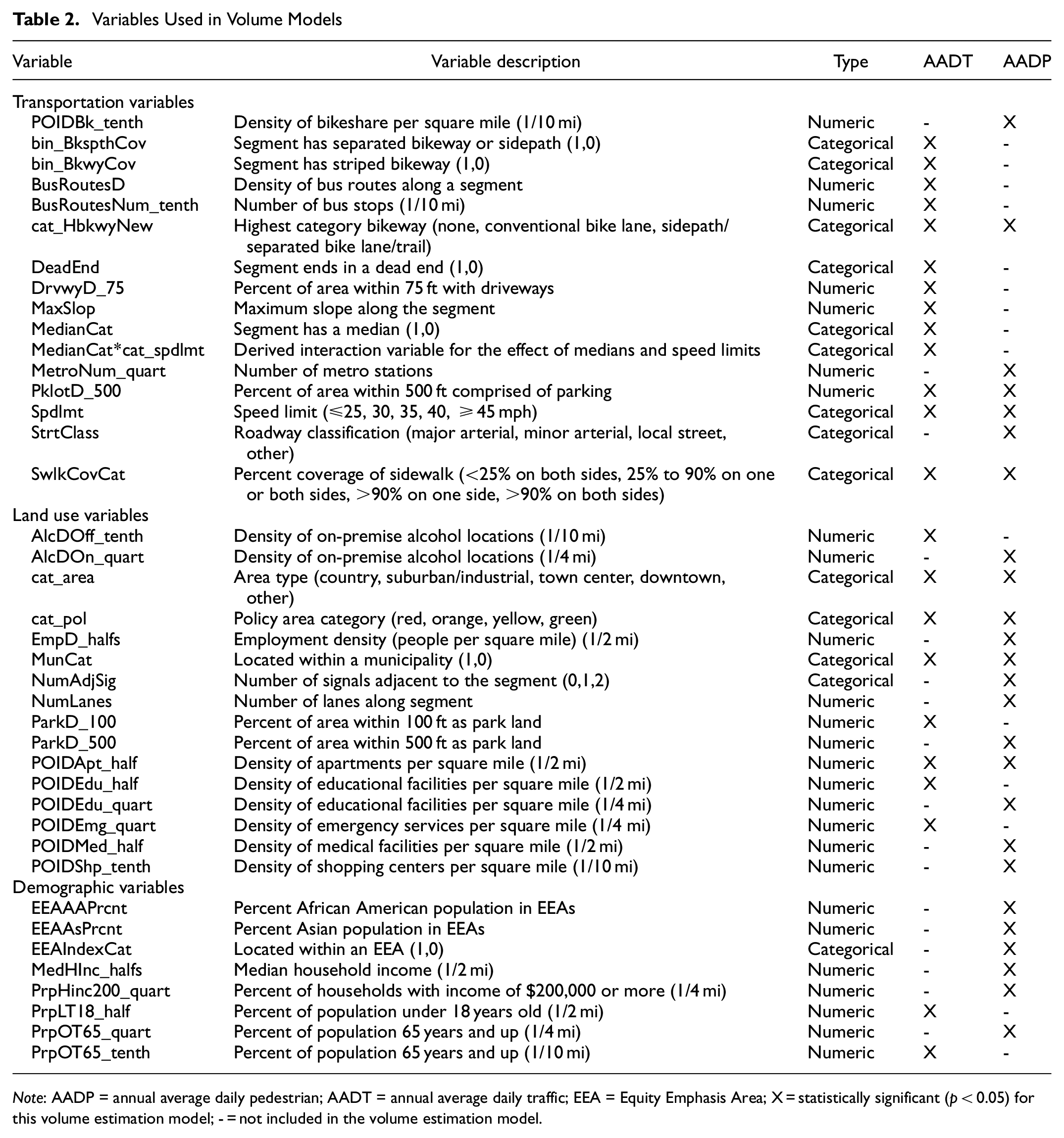
Note: AADP = annual average daily pedestrian; AADT = annual average daily traffic; EEA = Equity Emphasis Area; X = statistically significant (p < 0.05) for this volume estimation model; - = not included in the volume estimation model.
Statistically Significant Variables for both SPFs
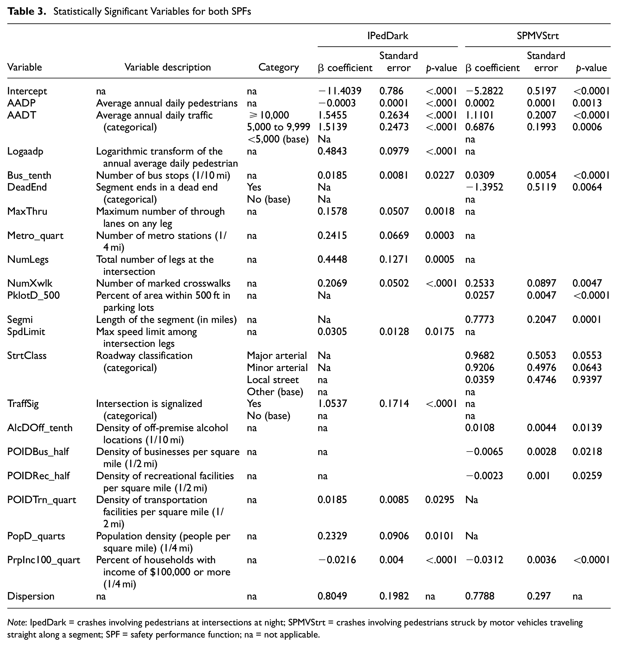
Note: IpedDark = crashes involving pedestrians at intersections at night; SPMVStrt = crashes involving pedestrians struck by motor vehicles traveling straight along a segment; SPF = safety performance function; na = not applicable.
Volume Estimation Models
The systemic safety approach relies on exposure data to give an accurate assessment of where pedestrians may be at risk on the roadway ( 4 ). Although SPFs can be calculated without taking pedestrian volumes into account, using only vehicular data may lead to missing important contextual information about where and how risks emerge in a system for pedestrians. To ensure that the models properly assessed risks, short-term multimodal counts were used to develop AADT and AADP estimates through a two-step process of count annualization and volume estimation.
The first step in developing the volume estimates was to adjust short-term counts (i.e., pedestrian counts taken at specific sites for between 1 h and 1 month) using temporal adjustment factors, including day-of-week-of-month-of-year and hourly factors ( 18 ). These factors were applied by travel pattern (e.g., commuter or recreational) using methodologies suggested by Johnstone et al. ( 19 ) and Miranda-Moreno et al. ( 20 ). The pedestrian temporal adjustment factors were calculated using continuous counts collected on two trails in Montgomery County and a trail in Arlington County, Virginia, with pedestrian traffic patterns like those in Montgomery County. Continuous counters maintained by the Maryland State Highway Administration on four roadways (two rural and two urban) in Fredrick, Howard, and Montgomery counties were used to calculate motor vehicle temporal adjustment factors.
After developing the temporal adjustment factors, the short-term counts for pedestrians and motor vehicles were expanded into segment-based AADT and AADP estimates. These estimates were then used as the dependent variables in log linear regression models to calculate AADT and AADP estimates for all segments in Montgomery County. After examining the statistical distribution of volumes along segments, negative binomial regression was selected as the best fit for the data. The generic form of a log linear model developed using negative binomial regression can be seen in Equation 1.

where
Developing each model included a three-step process. First, a regression technique called conditional random forest (CRF) was used to identify which of the numerical and binary variables in the dataset explained the variance. The “cforest” party package in R was used to generate regression trees that ranked the 142 input variables for potential explanatory power. Based on the CRF regression trees, 117 variables were retained for the AADP model and 70 for the AADT model, based on the program plotting these variables above a “zero importance” axis. Second, lower-importance variables (based on CRF results) were eliminated from highly correlated (i.e., r > 0.6) pairs using a correlation matrix, resulting in 53 variables for AADP and 42 variables for AADT. Third, Cook’s distance ( 21 ) was used to eliminate annualized-volume sites where the segment Cook’s distance exceeded three times the mean Cook’s distance on all segments ( 22 ). Finally, backward elimination was used to remove variables that were not statistically significant (p > 0.05) for each model.
The final AADT model consisted of 23 variables, and the final AADP model consisted of 25 variables. A full parameter discussion of the model results is beyond the scope of this paper, but the significant variables are listed by data type in Table 2. These models were used to estimate AADT and AADP on each road segment in the network. They were also used to estimate intersection volumes by summing the estimated AADT and AADP for all legs of each intersection and dividing the sum by two (because each motor vehicle and pedestrian enters and exits the intersection). To ensure that the best-fitting versions of the exposure variables were included in the SPFs, categorical versions of these exposure variables were developed; sometimes different functional forms of exposure variables may provide a slightly better fit ( 3 , 4 ). The exposure estimates were grouped into volume categories using three approaches: high and low categories; high, medium, and low categories; and five volume-group categories. The groups were roughly categorized by quantiles. When developing the SPFs, both categorical and numeric versions of all volume variables (i.e., AADT and AADP), as well as log-transformed versions of these variables, were tested in the negative binomial models to see which provided a better fit (based on cumulative residual [CURE] plots and other fit statistics). More information on the volume estimation models can be found in the final report for this project ( 8 ).
Safety Performance Function Development
Developing the two pedestrian SPFs followed a similar procedure to that used for the volume estimation step. First, a CRF analysis was performed using R on the crash type’s respective dataset, and any predictors with low CRF values were eliminated. This left 57 variables that were potentially explanatory for pedestrian dark (IPedDark) crashes and 87 that were potentially explanatory for segment collision (SPMVStrt) crashes. Second, a correlation matrix was developed for each crash type to eliminate lower CRF-scoring variables that were highly correlated. This process left 23 potential variables for the IPedDark regression model and 46 potential variables for the SPMVStrt regression model. Finally, backward elimination was used to remove variables that were not statistically significant (p > 0.05) for both crash types. Well-fitting models were compared by examining AIC (Akaike information criterion) and BIC (Bayesian information criterion) values ( 23 , 24 ). CURE plots were examined to assess overall model fit ( 25 , 26 ). Negative binomial regression was used, as suggested for SPF development in the Highway Safety Manual (HSM) ( 26 ). The SPFs took the form of the generic log linear equation shown in Equation 1. As mentioned, the statistically significant variables per SPF are shown in Table 3. Variables that were not included in one SPF are marked “na” for not applicable to that SPF.
Results
Crashes between Motor Vehicles and Pedestrians at Night at Intersections Model
The final dataset used to prepare the IPedDark crashes consisted of 16,594 intersections, with 23 potential variables considered for inclusion in the SPF. Proc Genmod in SAS version 9.4 was used to develop the SPF. Intersections were removed if they had missing categorical data or fewer than 2 years of crash data available; this last step was performed to ensure that there was more than 1 year of crash data per intersection to avoid modeling bias. The final intersection sample consisted of 16,387 intersections, and the final model retained 13 independent variables, shown in Equation 2.
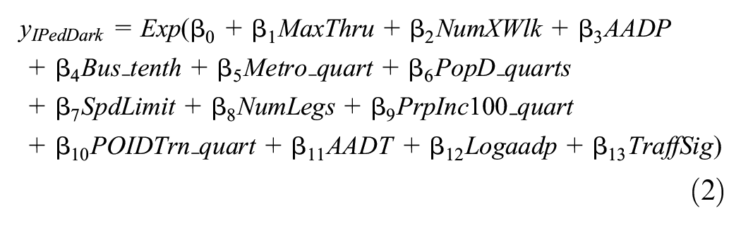
where
The AIC and BIC values for this IPedDark model were 2,333 and 2,456, respectively. The CURE plot shown in Figure 2 indicates a generally good model fit, with predictions lying within the upper and lower limits.
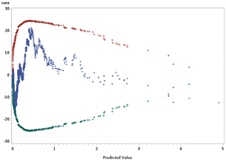
Cumulative residual (CURE) plot for the IPedDark model.
Table 3 shows the variable coefficients, standard errors, and p-values per variable. For this model, number of crash years was used as an offset, meaning that the model predicts total IntPedDark crashes per year.
The sign of the coefficients indicates the positive or negative relationship to IPedDark crashes. Maximum number of thru lanes, marked crosswalks, bus routes within a tenth of a mile, metro stations within a quarter of a mile, population density, speed limit, number of intersection legs, number of transportation facilities within a quarter mile, a logarithmic transform of AADP, medium or high AADT, and the presence of traffic signals were all positively associated with crash outcomes. These results indicated that the number of intersection crashes involving pedestrians at night tended to increase as traffic volume increased, as the number of bus stops nearby increased, as the number of thru lanes on any leg at an intersection increased, as the number of metro stations nearby increased, as the number of marked crosswalks at an intersection increased, as the speed limit increased, and as the population density and density of nearby transportation facilities increased. Generally, these results confirmed the crash risks identified in the study by Schneider et al. ( 11 ), namely that wide streets with higher speed limits are higher risk for pedestrians. Variables related to buses, metro stops, crosswalks, and traffic volume indicated the relation between crash risk and exposure, in that as more road users converge into single locations, the likelihood of a crash occurring increases.
AADP and the percentage of households with income above $100,000 were negatively associated with pedestrian crashes at intersections at night. The household income result may indicate some protective factor available to pedestrians in areas with higher household income, but more examination would be necessary to identify the relationship between household income and potential explanations like access to higher quality pedestrian facilities or greater vehicle usage. The negative sign of the AADP coefficient and the positive sign of the logarithmic transform of AADP coefficient may indicate that there is a curved relationship between pedestrian volumes and crashes.
This model contains three “typical” exposure variables: both AADP variables and AADT. Aside from speed limits, most of the predictive variables may be considered measures of exposure. The number of lanes and legs at intersections corresponded to the distances pedestrians needed to cross at night, whereas the other numeric variables gave a sense of where pedestrians may be more active and therefore more likely to be exposed to vehicular traffic.
Crashes between Motor Vehicles Traveling Straight and Pedestrians at Segments Model
The dataset for SPMVStrt crashes consisted of 30,613 segments before eliminating sites with missing categorical data or where there were fewer than 2 years of crash data available. This sample of segments included 46 potential explanatory variables. Through backward elimination in SAS, a sample of 29,715 segments and a model with 12 statistically significant (p < 0.05) variables were produced. The final segment SPF is shown in Equation 3, with parameter coefficients, standard errors, and p-values shown in Table 3.
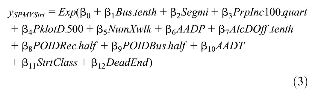
where
The AIC and BIC values for this SPMVStrt model were 3,230 and 3,371, respectively. The CURE plot shown in Figure 3 indicates a generally good model fit, with predictions lying within the upper and lower limits.
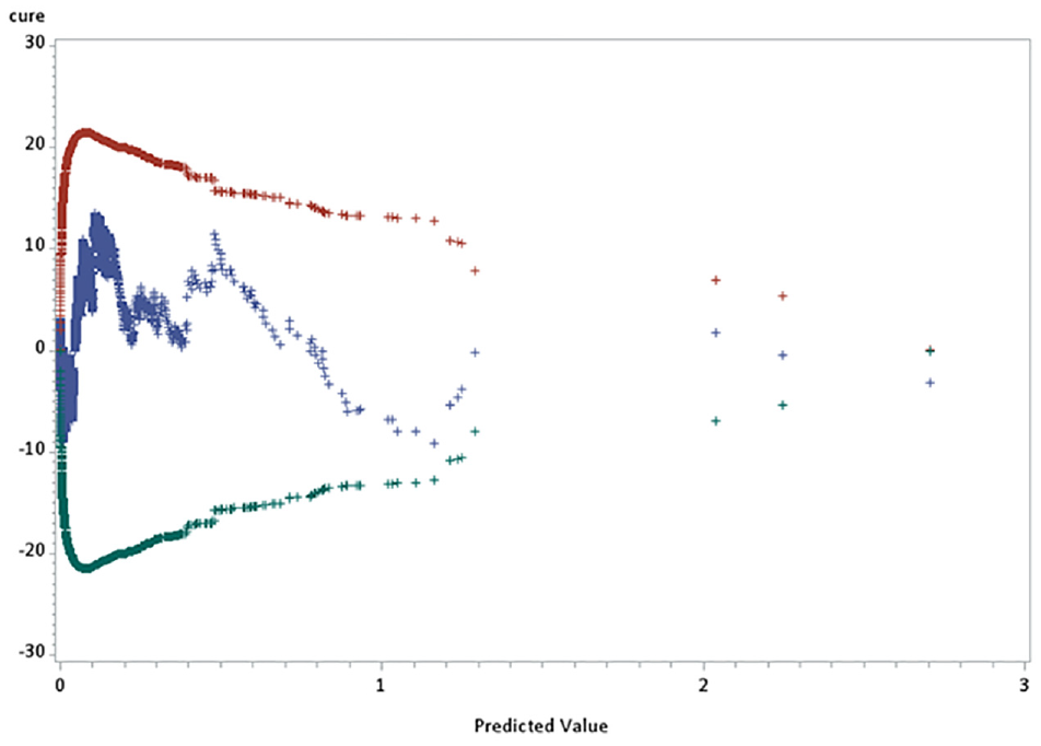
Cumulative residual (CURE) plot for the SPMVStrt model.
Numeric variables positively associated with SPMVStrt crashes included bus routes within a tenth of a mile, segment length, parking facility density, number of marked crosswalks (i.e., crosswalks that have at least pavement markings or more advanced markings and supportive infrastructure), AADP, and off-premise alcohol facility density within a tenth of a mile. Medium or high AADT values and all segment roadway classifications (compared with segments without classifications) were positively associated with crash outcomes. For roadway classifications, the major and minor arterials contributed most to the estimated crashes. These results indicated that the number of pedestrian crashes along a segment tended to increase as traffic volume increased, as the number of nearby bus stops increased, as the number of treated crosswalks on the segment increased, as the number of nearby parking facilities increased, and as the number of off-premise alcohol facilities increased. The parking facilities variable may indicate increased exposure to vehicular traffic or that the land use is oriented more toward automobile travel. The segment length variable may indicate that longer blocks are associated with more pedestrian crashes (and may be a surrogate for exposure) or that pedestrians may be unwilling to travel longer distances to cross at intersections. This finding is interesting because segment length is often used in prediction models to normalize crash prediction values ( 27 ), but here it is associated with segment crashes involving pedestrians. The numeric variable results showed that pedestrian risk tended to increase as roadways became larger (as indicated by the StrtClass variable) and as more road users converged onto segments.
The percentage of households with incomes greater than $100,000, recreational facilities within a half mile, business facilities within a half mile, and segment dead ends were negatively associated with pedestrian segment crashes. These results may indicate that in certain areas of Montgomery County, vehicular traffic may be lower or pedestrian traffic may be more expected, but more research into these factors is needed.
As with the IPedDark crash model, this model contains both typical exposure variables—AADP and AADT—and surrogate measures of exposure (e.g., segment length, roadway classification, number of treated crosswalks, and land use contexts). The roadway properties probably indicate that pedestrians are more likely to be struck on wide and long roadways between intersections, whereas the land use variables seem to indicate that pedestrians are less likely to be struck on segments adjacent to typical pedestrian activity attractors (e.g., businesses and recreation locations) or where motor vehicle traffic may be higher (e.g., near parking facilities).
Comparison of Top-Ranked Sites
MCPD can use the two SPFs to better understand pedestrian safety risks related to land use planning, Complete Streets street classifications, and EEAs. To aid in this assessment, the empirical Bayes methodology was applied following the procedure outlined in the HSM ( 28 ) to determine the number of expected vehicle–pedestrian crashes at intersections and segments. In the empirical Bayes procedure, the SPF was used first to estimate the number of crashes that would be expected at locations with traffic volumes and other characteristics similar to the one being analyzed. Then these predicted crashes from SPFs were combined with the count of crashes to obtain an estimate of the expected number of crashes at the site. In other words, an empirical Bayes method weights the crashes predicted using an SPF against observed crash histories and provides more accurate expectations of crashes that may occur ( 3 ) by properly accounting for the regression to the mean problem. Three different measures of safety were calculated across the whole network to identify types of locations with the highest crash risk. The measures for comparison are summarized in Table 4 and include
Total expected crashes: the sum of expected annual crashes for each crash type based on a defined geographical context.
High expected crash locations: the locations with the highest crash risk, specifically the top 200 intersections or segments for expected crashes per year for a given crash type.
Average expected crashes: the number of expected crashes per year divided by the number of locations for each crash type.
Crash Risk Summary
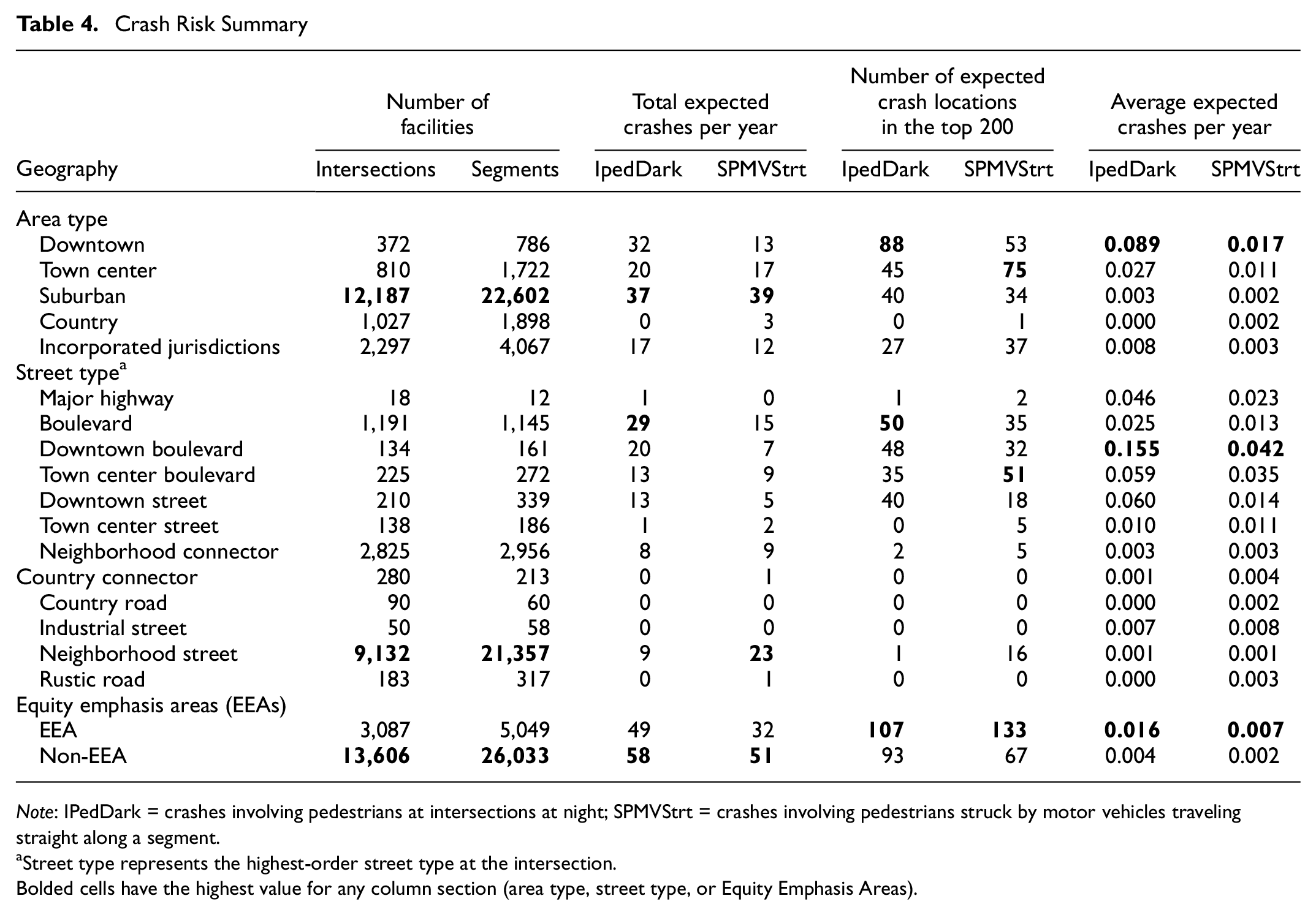
Note: IPedDark = crashes involving pedestrians at intersections at night; SPMVStrt = crashes involving pedestrians struck by motor vehicles traveling straight along a segment.
Street type represents the highest-order street type at the intersection.
Bolded cells have the highest value for any column section (area type, street type, or Equity Emphasis Areas).
MCPD identifies four land use contexts within unincorporated Montgomery County, from the most urban to rural: downtowns, town centers, suburban areas, and country areas. Given that most of the county is suburban in nature, the areas for the highest total expected crashes are in the county’s suburban communities. Yet in the high expected crash analysis, the focus shifts to the county’s urban areas, where 88 of the top 200 intersections for pedestrian crashes after dark at intersections were found in downtowns and 75 of the top 200 segments for pedestrian crashes along segments were in town centers.
The Montgomery County Complete Streets Design Guide ( 29 ) defines street types for different roadway classes throughout the county, ranging from major, limited access highways to low-speed neighborhood streets. For street types, total expected crashes varied across the two pedestrian crash types. Neighborhood streets, the most common street type in the county, were associated with the highest total expected crashes for pedestrians along segments. In contrast, the highest expected pedestrian crashes at intersections at night were along boulevards, the high-speed, high-volume arterials that connect the county’s urban centers. For the high expected crash analysis, boulevards and urban street types (downtown and town center boulevards and downtown streets) were the most frequent for both crash types: 173 of the top 200 locations for pedestrian crashes after dark and 136 of the top 200 locations for pedestrian crashes along segments occurred on these four street types. Downtown boulevards had the highest average expected crashes for both crash types.
Given that EEAs comprise just 18% of intersections and 16% of segments, it is not surprising that total expected crashes were higher in non-EEA areas in Montgomery County. However, EEAs were overrepresented relative to the number of intersections and segments in EEAs, as evidenced by more than half of the top 200 locations being within EEAs. Addressing this disparity requires focusing pedestrian improvements in the low-income communities and communities of color within Montgomery County. The disparity was most apparent in the evaluation of average expected crashes, where the average was higher in EEAs than non-EEAs by 270% for pedestrian crashes after dark at intersections and 226% higher for pedestrian crashes along segments.
The empirical Bayes results allowed the expected number of target crashes across all facilities in the roadway network to be compared and quantified as what percentage of each would occur at the top 200 high-risk locations. Of note is that although pedestrian-involved crashes after dark at intersections were relatively concentrated—with almost 50% of the expected crashes occurring within the top 200 locations—pedestrian crashes along segments with vehicles going straight were more dispersed throughout the county. Only 23% of the expected crashes with pedestrians along segments with motor vehicles going straight occurred in the top 200 locations. These analyses could support decision making and countermeasure selection so that limited safety project funding can be spent appropriately while addressing sites with the highest amount of risk. The next section identifies potential countermeasures that could be used as part of a systemic safety process.
Applications
Pedestrian Crash Countermeasure Selection
To determine appropriate countermeasures that could be applied systemically, the coefficients and distributions of each variable in both SPFs were examined in a sensitivity analysis and then compared to potential crash modification factors (CMFs) identified in the CMF Clearinghouse ( 30 ). CMFs are numerical factors or functions that, in the current version of the HSM, are applied to an SPF to estimate the change in predicted crashes per year should that countermeasure be implemented on a roadway facility. The CMF Clearinghouse lists multiple CMFs by treatment type and provides different ratings for the quality of the studies that produced those CMFs. CMFs may have values greater than or less than 1.0; a CMF with a value less than 1.0 indicates a reduction in crashes.
For pedestrian crashes at intersections in the dark, the most important variables for increasing the number of predicted crashes were all exposure related: presence of traffic signals, AADT, and AADP. These results present a challenge for a Vision Zero program in that Montgomery County would like to encourage continued use of pedestrian facilities and expand those facilities, especially in EEAs. Therefore, the countermeasure selection must focus on treatments that either reduce the severity of collisions when impacts do occur or improve pedestrian visibility and separation. Two potential treatments may include
Improving lighting: lighting may improve the visibility of pedestrians at nighttime, but the quality of related CMFs vary; Elvik and Vaa provide one CMF equal to 0.58 for nighttime vehicle–pedestrian crashes resulting in injuries ( 31 ).
Increasing pedestrian separation: signal timing measures may be effective at ensuring pedestrians are protected from vehicle traffic; Goughnour et al. reported lead pedestrian interval (LPI) CMFs equal to 0.81 and 0.83 for vehicle–pedestrian crashes ( 32 ).
The risks associated with pedestrians on segments were similar to those at intersections. The analysis identified more exposure-related variables, including high AADT, non-dead-end streets, and street classification, that seemed to correspond to a greater likelihood of a pedestrian being struck midblock. The risk treatment strategies for this crash type were like those at intersections. Potential countermeasures include
Reducing vehicle speeds: speed humps may be one treatment to lower speeds on appropriate roadway types; Elvik and Vaa reported a CMF equal to 0.6 for speed humps for all crash types that result in injuries on urban and suburban roadways ( 31 ).
Improving pedestrian crossing experiences: despite this study and others ( 3 ) showing a positive relationship between treated crosswalks and vehicle–pedestrian collisions, it is likely that crosswalk locations serve as surrogate exposure measures because those are simply the most desirable locations to cross along a segment; raised medians with or without marked crosswalks and pedestrian hybrid beacons (PHBs) may reduce vehicle–pedestrian collisions by 31.5% and 56.8%, respectively ( 33 ).
The listed CMFs are provided to illustrate the types of treatment that may address the types of risk that can be identified through systemic analyses. The pedestrian SPFs in this study demonstrated that specific land use contexts and other measures of exposure to risk are critical to understanding where pedestrian crashes occur, so systemic treatments can then be applied, as appropriate, at those types of locations to address the common causes of severe crashes for pedestrians using the roadway, namely coming into conflict with vehicular traffic, especially at high speeds ( 11 ).
Vision Zero Countermeasure Evaluation Tool
This study’s analysis did not result in a prescriptive recommendation of capital improvements; it does not recommend which countermeasures should be implemented at which locations. Instead, the project describes the development of a model-based risk assessment and a countermeasure evaluation process and provides a tool for planners, engineers, and decision makers to assess different investment scenarios based on their goals and priorities.
The tool evaluates the effectiveness of different countermeasure scenarios through several metrics: potential crash reduction, potential crash reduction per location, cost per crash reduction (based on local unit costs), and percent of locations in EEAs. Safety improvements should be prioritized in the places where they are most needed. As a result, the countermeasure evaluation tool applies countermeasures to the top-ranked locations for each countermeasure based on its empirical Bayes expected crash estimate.
Each of the countermeasures are associated with a ranked list of locations for systemic implementation. However, given the countywide nature of this analysis, individual site reviews are needed to confirm that the identified countermeasures are context-appropriate for the selected sites. To illustrate how systemic countermeasures may result in improved crash reduction across a network, an example scenario of a crash treatment based on a fixed budget is provided.
Example Scenario: Determining Which Countermeasures to Implement
This scenario demonstrates how a jurisdiction might determine the best use of a limited budget to treat target crashes identified through a Vision Zero program and as described in the systemic pedestrian safety literature ( 3 ). This scenario assumes a countermeasure budget of only $200,000 and a goal to decrease pedestrian crashes along segments. Assuming a 10-year analysis period, Table 5 shows the 1-year and long-term benefit of constructing midblock crosswalks, speed humps, or a PHB.
Example Scenarios for Reducing Pedestrian Crashes along Segments with $200,000
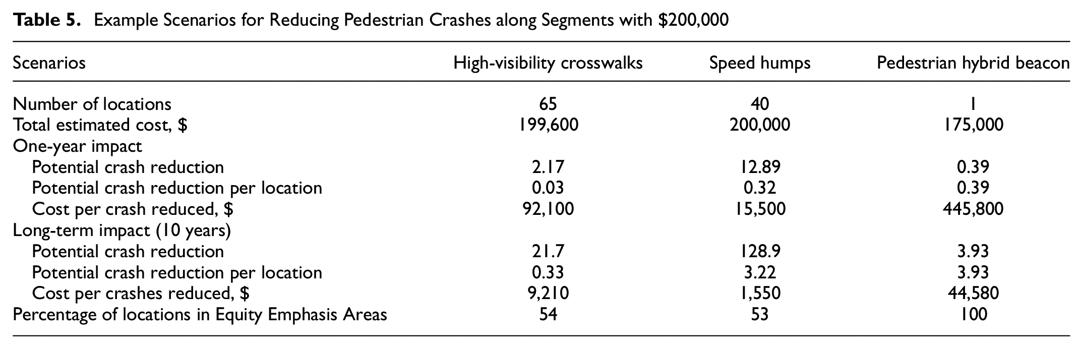
As countermeasures vary in their costs, how many locations can be addressed with $200,000 differs across the countermeasures. Updating marked crosswalks and constructing speed humps are far less costly than a PHB, so many more locations could be updated with this treatment (65 and 40 locations, respectively, versus 1 location). Given the CMF and the number of locations addressed, the potential crash reduction for constructing speed humps far exceeds the other treatments, yet the per-location crash reduction is lower than that of constructing a PHB.
Conclusions
This paper presents the results of a comprehensive systemic safety analysis to compile data, model key high-severity crashes, and identify locations for treatment as part of a countywide Vision Zero program. This paper contributes an SPF for crashes involving pedestrians at intersections at night and a segment-based SPF for crashes involving pedestrians along segments. The intersection SPF demonstrated the importance of intersection size (via independent variables like the number of legs and lanes and the number of marked crosswalks) and design (via independent variables like the maximum speed limit at the intersection) for pedestrian exposure to risk. These variables indicated the kinds of intersections in Montgomery County where pedestrians are likely to come into contact with motor vehicles and could help practitioners in determining where to apply countermeasures that could increase pedestrian separation (e.g., through LPIs or refuge islands) or that might increase visibility where crashes are likely to occur. The segment SPF verified some of the findings reported for this crash type in the literature ( 4 ).
This study also demonstrated the importance of data collection as part of a systemic safety process and demonstrated a countywide application of systemic safety procedures. Complete, accurate data are crucial for any analysis, and missing data may limit model applications. For example, Montgomery County lacks a comprehensive dataset for signal timing, but cycle length, inclusion of a protected or protected/permissive left-turn phase, or leading pedestrian intervals are potentially significant variables related to pedestrian crashes at intersections. Moreover, countywide data are not available about where turn lanes are present or whether those turn lanes are channelized. Without knowing where these intersection characteristics are present, Montgomery County cannot systematically evaluate the benefit of implementing these treatments at applicable locations.
This analysis is the first step toward implementing a proactive approach to pedestrian safety in Montgomery County. Based on the findings and tools developed, the Planning Department, Montgomery County Department of Transportation, and the County Council can use this information in a variety of ways to inform future recommendations, prioritize projects, and allocate funding. Key takeaways include the need to
Apply data-driven planning: Historically, much of transportation planning has been reactive. This study provides the data, analysis, and tools to shift the County’s approach and implement improvements where they are needed and more equitably. The data could support funding requests, both as part of the local or state budgeting process as well as through grant applications.
Identify locations with high expected crashes: The results of this study could be used to identify location types that are at greater risk of a high number of crashes and may inform Capital Improvement Program (CIP) project prioritization, risk mitigation for new developments, and long-term transportation improvements within master planning areas.
Prioritize safety improvements: The countermeasure evaluation tool demonstrated in this study will allow implementing agencies to prioritize where to implement systemic safety treatments as well as to assess which safety treatments, with some limitations, may be the most effective at reducing crashes systemically. This information could make the case for additional funding for CIP level-of-effort programs and inform master plan recommendations.
These broad uses could be applied to several aspects of transportation planning, engineering, funding, and implementation, as listed in the examples above. Over the longer term, a systemic approach to crash prediction could also help facilitate the redesign of the entire transportation network, by identifying road designs, populations, and land use patterns that are associated with risk and mitigating that risk through new policies and systematic designs. Taking a more proactive, data-driven approach to transportation safety will have an impact on all facets of the transportation planning process.
Despite this study’s potential impacts on safety in Montgomery County, there were some limitations to the analysis. As mentioned, some data variables, such as signal timing and turn lane designations, were missing in the compiled dataset, whereas other data, such as the sidewalk inventory, had missing data that required broader categorizations than initially intended. Addressing these data limitations may enable practitioners to more accurately identify pedestrian risks and potential countermeasures. The SPFs themselves were also data-intensive to develop, and other jurisdictions may lack the technical resources to develop their own versions of these models, so calibration would be required before these models could be applied to other jurisdictions. Additionally, negative binomial regression models have some limitations and may not properly account for all differences between sites, and since the completion of this project, alternative modeling approaches have been suggested to account for site heterogeneity. A follow-on study using one of these methods, such as random parameters negative binomial regression ( 34 ), may be an option to update the County’s crash predictions if they provide a better fit than the current models based on criteria like AIC and BIC. However, as with other large-scale systemic risk models ( 5 , 6 ), the risk factors identified through this analysis could be adapted for use in weighted models and may assist other practitioners in identifying sites of concern across other roadway networks.
Footnotes
Acknowledgements
The authors would like to acknowledge Dan Gelinne, Taha Saleem, and Rebecca Sanders of the project team, who were not involved in preparing this manuscript.
Author Contributions
The authors confirm contribution the paper as follows: study conception and design: K. Nordback, W. Kumfer, J. McGowan, L. Thomas; data collection: M. Vann, W. Kumfer, K. Nordback, J. McGowan, B. Frizzelle, L. Thomas; analysis and interpretation of results: W. Kumfer, K. Nordback, J. McGowan, B. Lan, M. Vann, L. Thomas; draft manuscript preparation: W. Kumfer, J. McGowan, K. Nordback, M. Vann, B. Lan, L. Thomas, B. Frizzelle. All authors reviewed the results and approved the final version of the manuscript.
Declaration of Conflicting Interests
The authors declared no potential conflicts of interest with respect to the research, authorship, and/or publication of this article.
Funding
The authors disclosed receipt of the following financial support for the research, authorship, and/or publication of this article: This project was performed under the Montgomery County Planning Department project “Vision Zero Predictive Safety Analysis” and funded by the Maryland-National Capital Park and Planning Commission (Sponsor Award Number P40-132 536097).
The contents of this paper do not reflect the opinions of Montgomery County.