Sage Journals: Discover world-class research

Abstract

Freight transportation plays a crucial role in sustaining the Canadian economy. However, heavy truck transportation also puts enormous pressure on roadway networks. Spring Load Restrictions (SLR) are implemented to minimize road damage caused by heavy traffic during the thaw-weakening season, and Winter Weight Premium (WWP) is used to reduce the impact of SLR on trucking operations by allowing higher axle loads in winter. However, existing policies apply fixed dates each year for these restrictions, regardless of the actual structural capacity of the pavement. Different methods have been proposed to improve the application of SLR and WWP; however, they rely mainly on indirect indices, such as the cumulative thawing index and cumulative freezing index, which pose challenges in their calculation. This study explores the practical implementation of machine learning models for accurately determining the start and end dates of SLR and WWP. In a novel approach, machine learning models directly derive the start and end dates of SLR and WWP from frost and thaw depths in the pavement structure which are determined by pavement temperature and moisture content. In contrast to previous studies that neglected the influence of soil moisture content on determining the start and end dates of SLR and WWP, this study examines the variation in soil moisture content to evaluate the validity of existing theories. The findings reveal a high level of agreement between the machine learning model’s estimations of frost and thaw depths and the measured values, with R² values exceeding 0.91.

Keywords

spring load restrictions winter weight premium frost depth thawing depth machine learning

Freight transport plays a crucial role in sustaining Canada’s economy, but the substantial volume of heavy truck traffic places immense pressure on the country’s roadway networks. This pressure can lead to premature failure, extensive pavement damage, the need for costly road maintenance, and other related issues if exceeding the design criteria. Furthermore, Canada’s cold regions present additional challenges for roadways, including frost heave, freeze–thaw cycles, and thawing weakening. In late winter and early spring, the temperature of the pavement structure rises from top to bottom, resulting in the upper soil layer thawing and the lower layer remaining frozen, leading to limited drainage capacity. The water in the subgrade layer cannot be discharged in time, resulting in a significant increase in water content. Moisture content influences the density and modulus of both the soil and bound materials, ultimately affecting the overall performance of the pavement (1 –6). Soil reaches its maximum density at an optimum moisture content. If all other conditions remain the same, both coarse-grained and fine-grained materials can significantly increase their modulus when dry, often by more than five times. Thus, the high moisture content in the spring can cause a decrease in the stiffness of the subgrade. On the other hand, excess water can lead to the separation of the asphalt binder from the aggregate, resulting in long-term effects on the structural integrity of the cementitious material. As a result, roadways become more vulnerable to the detrimental effects of heavy truck traffic, further exacerbating the strain on the infrastructure (7 –10).

To mitigate the damage caused by excessive truck loads to roads during the thaw-weakening season, authorities in North America employ Spring Load Restrictions (SLR) to impose load limits on roads. However, the use of SLR poses economic challenges for the local freight transportation industry. To address the economic difficulties faced by the trucking industry during the thaw-weakening period, the Winter Weight Premium (WWP) has been introduced. This involves increasing the maximum allowable axle load during the freezing period. Many authorities apply a fixed date every year; however, the fixed-date approach fails to consider the actual load-carrying capacity of the pavement, potentially resulting in inefficient restrictions or inadequate protection for the roads ( 11 ). Asefzadeh et al. conducted a study in which they collected two years’ pavement temperatures from a test road in Edmonton, Alberta, and calculated the actual frost and thaw depths ( 12 ). The results indicated variations in the frost progress and thawing duration between the two years, highlighting the year-to-year variability of the start and end dates of SLR and WWP. These findings underscore the need for a dynamic approach that replaces the traditional fixed-date approach.

Previous studies (13 –15) have relied on indirect parameters, such as cumulative thawing index (CTI) and cumulative freezing index (CFI) to estimate the start and end dates of SLR and WWP. CTI is a crucial parameter and is generally defined by the following equation:

CTI = \sum^{(T_{avg} - T_{r})}

(1)

Here, T_r represents the average air temperature when the asphalt temperature fluctuates around 0°C. As the days become longer during late winter and early spring, T_r decreases as a result of increased solar radiation absorption by the asphalt layer, causing pavement layers to thaw at lower ambient air temperatures. Mahoney et al. recommended using a fixed T_r value of −1.67°C ( 15 ). Additionally, CFI represents the accumulated degree days below the base temperature, and it is expressed as Equation 2:

CFI = \sum^{(T_{b} - T_{avg})}

(2)

Here, T_b is the base temperature and because T_b represents a threshold temperature below which the accumulation of freezing degree days is considered, the choice of the base temperature depends on the application and the specific characteristics of the system being analyzed. In pavement engineering, common values for the base temperature are often set at 0°C or some other temperature close to the freezing point of water. These indices reach a threshold, triggering the application of SLR or WWP. However, these studies lack a clear definition of the end date of SLR, and the calculation of the CTI and CFI poses significant challenges ( 12 ). Determining the start date of the CTI calculation is difficult because of unexpected increases in winter air temperature (e.g., in January and February). Moreover, the CTI and CFI calculations require calibration with a reference temperature specific to each location.

Asefzadeh et al. utilized three existing models to measure the CTIs and estimate the start and end dates of SLR for a test road in Alberta ( 12 ). The predicted start dates of SLR showed a variation of two to four days among the models. However, the differences in the predicted end dates of SLR were unacceptably large, exceeding one and a half months. Additionally, all three existing methods suggest removing SLR before the soil moisture content recovers from the high-water levels.

Baïz et al. and Bao et al. proposed theories to determine the start and end dates of SLR and WWP based on frost and thaw depths (16 –18). However, these depths were also calculated using freezing and thawing indices. Moreover, the existing pavement temperature prediction models in the literature (19 –22) are limited to the asphalt layer. The proposed theories (16 –18) also failed to consider the soil moisture content. To date, no research has addressed the direct estimation of SLR and WWP application and removal dates through pavement temperature. Thus, a new method that dynamically determines the start and end dates of SLR and WWP based on frost and thaw depths derived from pavement temperature can improve road management.

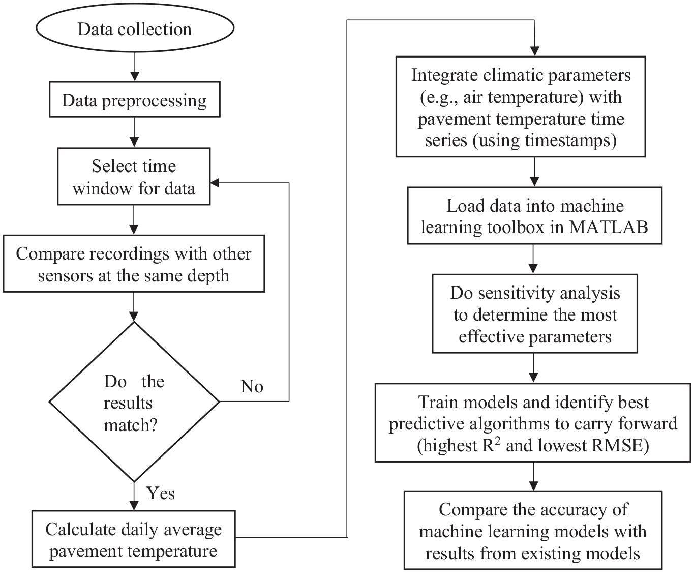
In recent years, machine learning (ML) models have gained popularity for estimating environmental factors of pavement structure, including pavement temperature ( 20 , 23 –27) and moisture content ( 28 ) at different depths using available inputs. Building on this trend, the primary aim of this study is to introduce a dynamic approach, ML models, to determine the start and end dates of SLR and WWP based on predicted frost and thawing depths. The ML models dynamically determine SLR and WWP dates by integrating timely collected air temperature data. The ML model was developed by pavement temperatures collected from the Integrated Road Research Facility (IRRF) test road from January 2013 to December 2020.

Additionally, this study aims to assess the validity of existing theories that determine the start and end of SLR and WWP based on frost and thaw depths by comparing the model’s outcomes with changes in moisture content in the subgrade. To achieve this, pavement temperatures and moisture content measured from the IRRF test road during specific periods, including November 2013 to August 2014 and November 2016 to August 2017, were utilized. By employing this dynamic approach, the research seeks to enhance the accuracy and effectiveness of SLR and WWP implementation, enabling road authorities to make informed decisions based on real-time data and subgrade conditions. The comparison between the ML model and water content variations in the subgrade provides valuable insights into the applicability and reliability of existing theories in determining the appropriate timing for implementing and lifting SLR and WWP. This analysis contributes to advancing our understanding of the factors influencing road damage during the thaw-weakening season and aids in the development of more robust and efficient policies for managing truck transportation. Ultimately, by refining the methodologies for determining SLR and WWP dates, this research aims to promote sustainable freight transport practices and minimize the negative impacts of low-load structural capacity during the thawing-weakening period on roadway networks.

Machine Learning Model Development

Data Characteristics

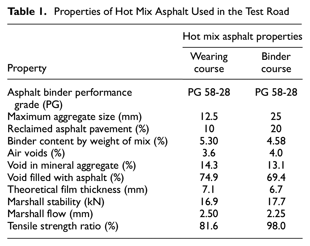
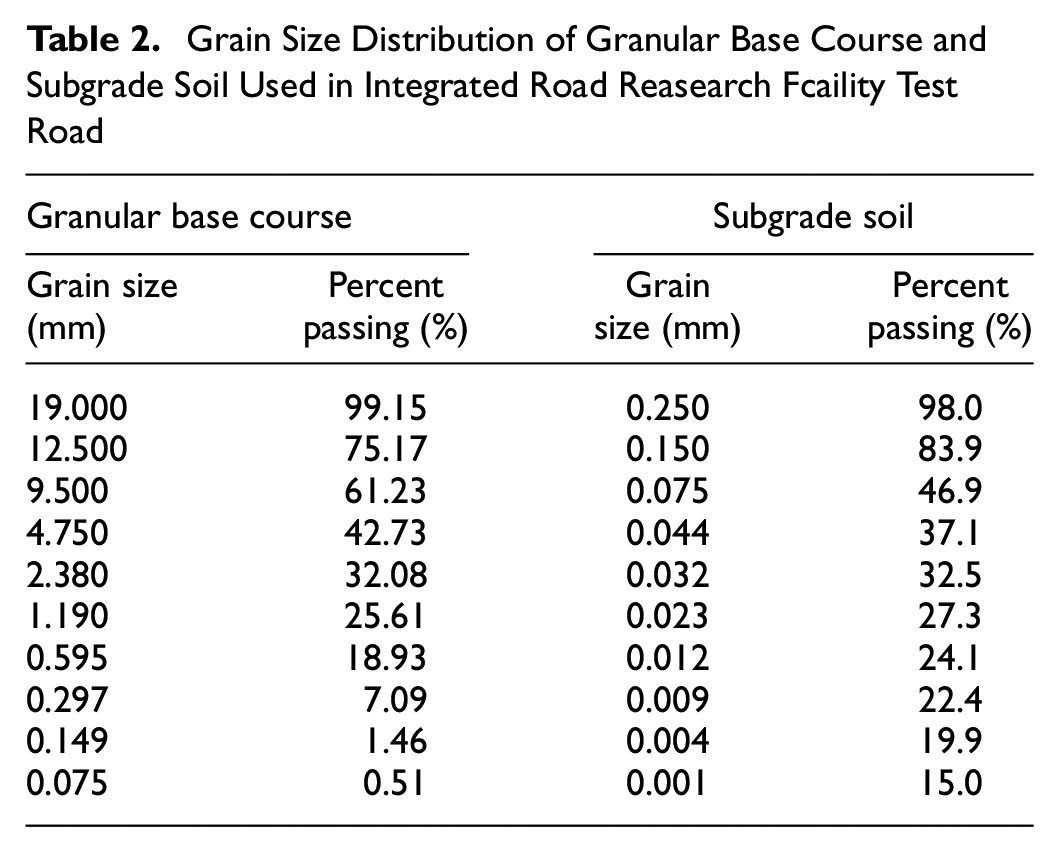
The IRRF test road, located in Edmonton, Alberta, serves as an advanced instrumented test road designed to investigate the environmental influence on pavement structure performance. Construction of the IRRF test road commenced in 2012 and was completed in 2013, and it opened to public traffic in 2015. Figure 1 illustrates the composition of the test road, which comprises a 0.25 m layer of hot mix asphalt (HMA) placed on top of a 0.45 m granular base course (GBC). Table 1 lists the physical properties of HMA mixes used in the IRRF test road. Table 2 provides the grain size specifications for the GBC and subgrade soil. The GBC is composed of well-graded gravel, with a maximum particle size of 0.019 m and a density of 2.10 ton/m³. The subgrade soil, classified as clayed sand, has a maximum particle size of 0.0005 m and a density of 1.85 ton/m³. The liquid limit of the subgrade soil is 25% and the plasticity index is 9%.

Figure 1.

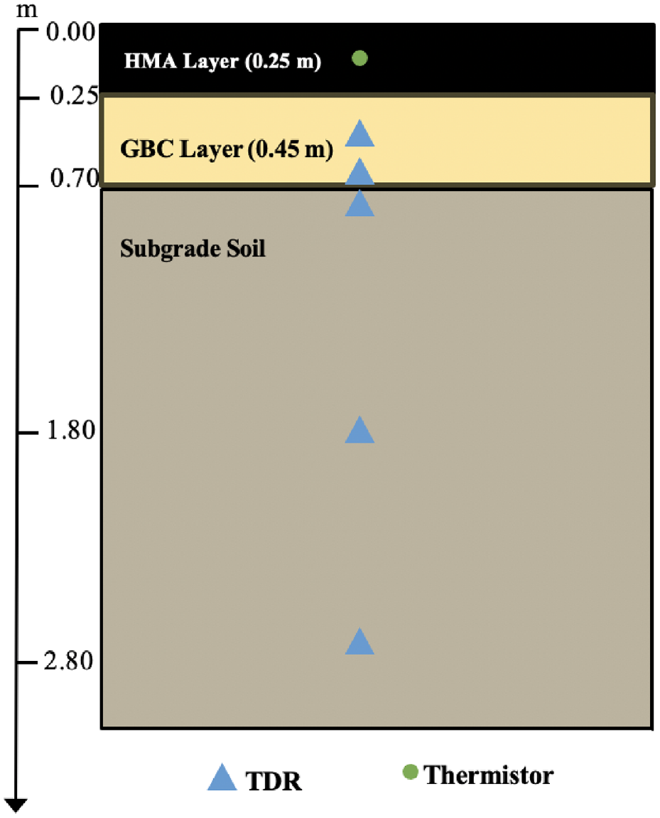
Cross-section of the Integrated Road Reseach Facility test road.

Table 1.

Properties of Hot Mix Asphalt Used in the Test Road

Property	Hot mix asphalt properties
Property	Wearing course	Binder course
Asphalt binder performance grade (PG)	PG 58-28	PG 58-28
Maximum aggregate size (mm)	12.5	25
Reclaimed asphalt pavement (%)	10	20
Binder content by weight of mix (%)	5.30	4.58
Air voids (%)	3.6	4.0
Void in mineral aggregate (%)	14.3	13.1
Void filled with asphalt (%)	74.9	69.4
Theoretical film thickness (mm)	7.1	6.7
Marshall stability (kN)	16.9	17.7
Marshall flow (mm)	2.50	2.25
Tensile strength ratio (%)	81.6	98.0

Table 2.

Grain Size Distribution of Granular Base Course and Subgrade Soil Used in Integrated Road Reasearch Fcaility Test Road

Granular base course		Subgrade soil
Grain size (mm)	Percent passing (%)	Grain size (mm)	Percent passing (%)
19.000	99.15	0.250	98.0
12.500	75.17	0.150	83.9
9.500	61.23	0.075	46.9
4.750	42.73	0.044	37.1
2.380	32.08	0.032	32.5
1.190	25.61	0.023	27.3
0.595	18.93	0.012	24.1
0.297	7.09	0.009	22.4
0.149	1.46	0.004	19.9
0.075	0.51	0.001	15.0

Pavement temperature and moisture content data were collected using CS650 time domain reflectometers (TDRs, Campbell Scientific). The TDRs recorded the pavement temperature and volumetric water content (VWC) at depths of 0.50, 0.70, 0.80, 1.80, and 2.70 m below the road surface at 5 min intervals. The TDRs employed the Topp equation ( 29 ) to calculate VWC based on the bulk dielectric permittivity of the soil (K_α):

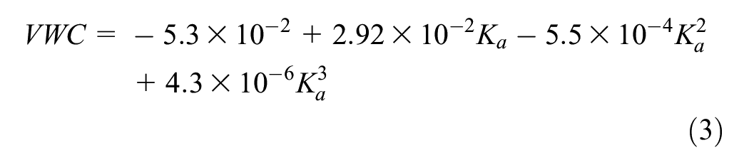
\begin{matrix} VWC = & - 5.3 \times 10^{- 2} + 2.92 \times 10^{- 2} K_{a} - 5.5 \times 10^{- 4} K_{a}^{2} \\ + 4.3 \times 10^{- 6} K_{a}^{3} \end{matrix}

(3)

where VWC (m³/m³) is the volumetric water content, and K_α is the bulk dielectric permittivity of the soil. The speed of wave propagation depends on the dielectric permittivity of the porous medium. Increasing the water content reduces the speed of propagation or increases the time it takes for an electromagnetic wave to travel from one pole to another. This dependence has led to naming the probe the “Time Domain Reflectometer.” Laboratory tests were conducted to calibrate the VWC using soil samples collected from the IRRF test road. The permittivity of water is influenced by temperature and water is the main contributor to soil permittivity, so the soil permittivity is temperature dependent. Equation 4 ( 7 ) was used to eliminate the temperature dependency of the measured results:

VW C_{21} = VWC / (0.0084 (T - 21) + 0.9936)

(4)

where 21°C was used as the base point to calibrate the permittivity, VWC₂₁ (m³/m³) represents the soil permittivity without the effect of temperature, and T (°C) is the temperature of the sample. Meanwhile, soil permittivity is influenced by soil type and the compaction of the soil. Calibration was also performed for the GBC and subgrade materials using Equations 5 and 6 ( 7 ).

VW C_{GBC} = 1.338 VWC - 0.0901

(5)

VW C_{subgrade} = 1.1619 VWC - 25.296

(6)

where VWC_GBC (m³/m³) is the volumetric moisture content of the GBC layer and VWC_subgrade (m³/m³) is the volumetric moisture content of the subgrade layer. It is important to note that the TDRs only captured variations in liquid water content during spring ( 4 ).

Model Development

The ML model was developed using the average daily pavement temperature data collected from the IRRF test road, as shown in Figure 2. Pavement temperature data were collected from January 2013 to December 2020, and the details are provided in Table 3. The environmental parameters—such as average air temperature, solar radiation, and other relevant factors—were collected from the nearest Environment Canada weather station, Oliver AGDM.

Figure 2.

Procedure for developing machine learning predictive models ( 23 , 28 ).

Table 3.

Performance of the Machine Learning Model Developed

Depth (m)	Start date	End date	Number of daily average temperatures (processed)	Machine learning
Depth (m)	Start date	End date	Number of daily average temperatures (processed)	R ²	RMSE (°C)
0.50	January 2013	June 2020	1849	0.98	1.70
0.70	January 2013	July 2020	1769	0.98	1.80
0.80	January 2013	December 2019	1554	0.98	1.62
1.80	January 2013	August 2020	1904	0.98	1.20
2.70	January 2013	December 2017	1402	0.98	0.76

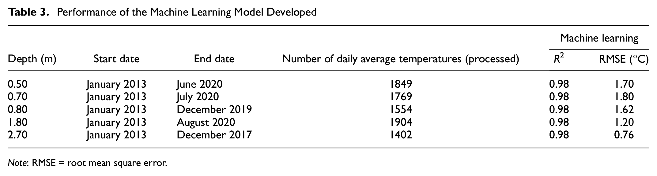
Note: RMSE = root mean square error.

A sensitivity analysis was conducted to assess the correlation between the pavement temperature and different parameters, and the performance of various parameter combinations was compared. Correlation coefficients were calculated between pavement temperature and other parameters to identify the most efficient input parameters. Day of the year and air temperature showed higher values (0.96 for the day of year and 0.93 for air temperature) than other input parameters, indicating they are the most significant input parameters. Then, the performance of various parameter combinations was compared. Among the analyzed parameters, the best combination identified for input parameters was average air temperature, day of the year, and depth. Day of the year serves as a time-related parameter ranging from 1 to 365, with January 1st corresponding to the value of 1. Depth is used to locate the sensors. Detailed information about the sensitivity analysis can be found in the previously published study ( 22 ).

For the model’s development, the ML toolbox regression learner, in MATLAB version R2017a, was utilized. All five ML algorithms available in the toolbox, namely regression trees, support vector machines, Gaussian process regression models, ensembles of trees, and linear regression models were employed to train the models. The performance of the ML models was evaluated using the coefficient of determination (R²) and the root mean square error (RMSE). Equations 7 and 8 were used to calculate R² and RMSE:

R^{2} = 1 - \frac{\sum_{i} {(x_{i} - f_{i})}^{2}}{\sum_{i} {(x_{i} - \bar{x})}^{2}}

(7)

RMSE = \sqrt{\frac{\sum_{i = 1}^{N} {(x_{i} - f_{i})}^{2}}{N}}

(8)

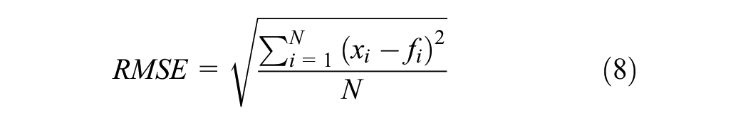
where x_i represents the actual value, f_i represents the predicted value, $\bar{x}$ is the mean value of the entire dataset, and N is the total number of data points.

The choice of the regression learner toolbox in MATLAB was based on several factors. ML techniques have demonstrated significant success in various engineering applications, including pavement temperature prediction. The regression learner toolbox in MATLAB is a versatile and widely used platform that offers a range of ML algorithms suitable for regression tasks. The decision to use this toolbox was influenced by its user-friendly interface, extensive documentation, and compatibility with the specific requirements of the study.

Moreover, regression learner has been successfully applied in previous studies to predict pavement temperature in asphalt, showcasing high accuracy and reliability. This track record of success further supported the suitability of regression learner toolbox in MATLAB for model development.

Among the ML algorithms used, most demonstrated excellent performance achieving R² values above 0.95, except for the linear regression model. The linear regression model is a widely used algorithm, but it assumes a linear relationship between input parameters and the target variable, which does not hold for pavement temperature prediction.

The Gaussian process regression ML model stood out as the top performer, exhibiting the highest accuracy with an impressive R² of 0.99 and an RMSE of 1.45°C for temperature prediction at all the five depths. Table 3 demonstrates the performance of the Gaussian process regression model at each depth. As can be observed, the pavement temperature variation is more significant at the shallower depths than that at the deeper locations, like depths of 1.80 m and 2.70 m, thus the RMSE is smaller at deeper locations. Gaussian process regression is a nonparametric Bayesian method that employs Gaussian processes for regression. Gaussian process regression calculates the probability distribution over all acceptable functions that can ﬁt the given data. The superiority of Gaussian process regression models in estimating pavement temperature can be attributed to their ability to capture complex relationships without relying on strong assumptions, handle small or sparse datasets effectively, and provide uncertainty estimates. The flexibility, probabilistic nature, and ability to handle uncertainty make Gaussian process regression models well suited to the specific task of pavement temperature estimation ( 30 , 31 ). Cross-validation was employed to validate the performance of the ML model, with the data randomly divided into five groups. The available testing data were randomly divided into five groups for cross-validation, with four groups used for training and the remaining group used for testing in each iteration. This process was repeated five times, and the average test error was calculated over all folds. This approach serves as a form of regularization by providing a more robust assessment of the model’s performance and generalization capability. All the estimated pavement temperatures presented in this study were calculated by the Gaussian process regression ML model ( 18 ).

Air Temperature

Air temperatures were collected from the Oliver ADGM weather station. Figure 3a represents the average daily air temperature, whereas Figure 3b shows the average monthly air temperature. The data cover the period from November to May for the years 2013 to 2014 and 2016 to 2017.

Figure 3.

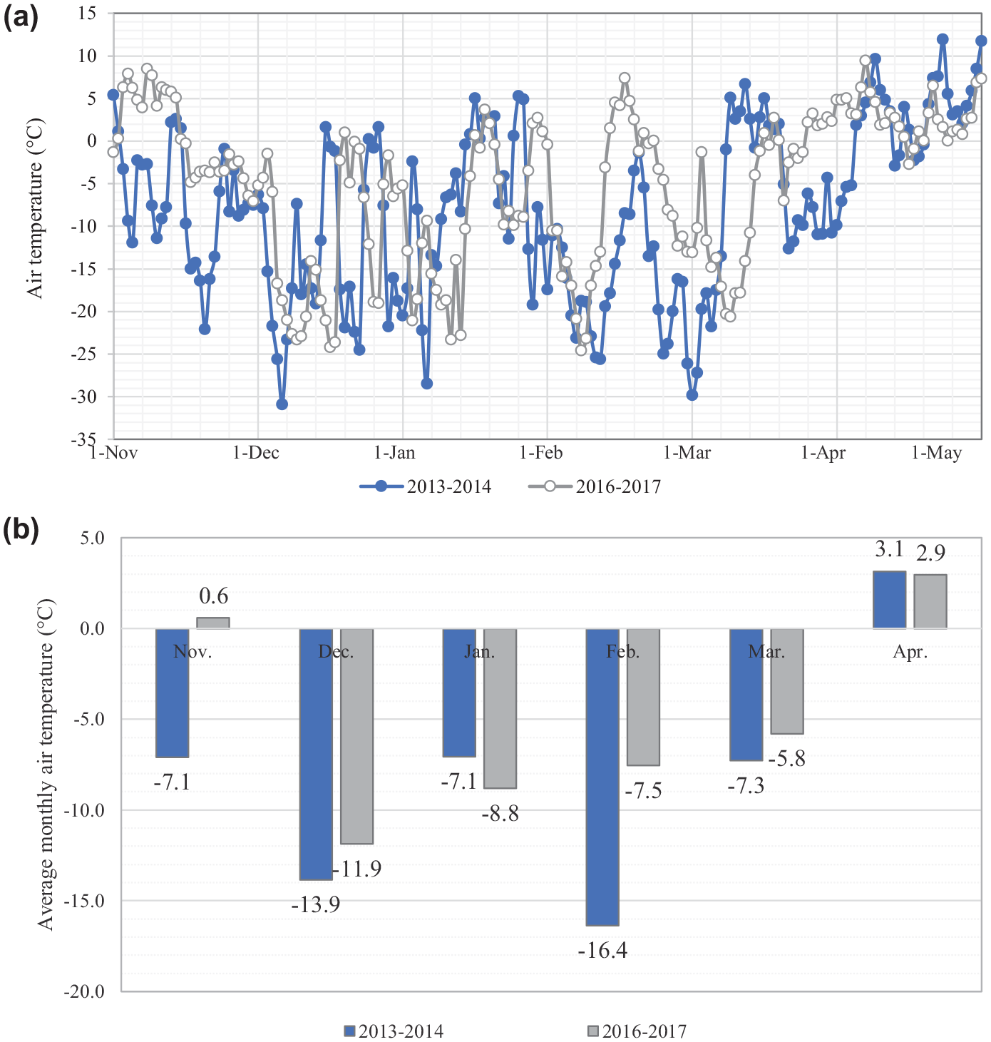
(a) Average daily air temperature and (b) average monthly air temperature.

In the winter of 2013 to 2014, the average daily air temperature dropped below 0°C from November 3, 2013. The lowest average daily air temperature recorded during this period was −30.9°C on December 6, 2013. The average daily air temperature remained below 0°C until March 9, 2014, with occasional days in December and January when the average daily air temperature reached above 0°C. The average monthly air temperature for February 2013 was −16.4°C whereas it was −7.5°C for February 2017, indicating consistently cold temperatures during that month.

Comparatively, the winter of 2016 to 2017 experienced milder weather. The average daily air temperature remained above 0°C until November 15, 2016, and then stabilized below 0°C to March 18, 2017. In November 2016, the average monthly air temperature was still above 0°C, whereas in 2013 the average monthly air temperature was −7.1°C. From December to April, the average monthly air temperature remained below 0°C, although the average monthly air temperature values for December, February, and March in 2017 were higher than those recorded in 2014.

Comparison of Measured and Estimated Frost and Thawing Depths

In the frost and thaw depth analysis, interpolation is based on measured and estimated temperatures at different depths. Figure 4 compares the measured frost and thaw depths obtained from sensors installed in the test road, with the estimated frost and thaw depths calculated using the Gaussian process regression ML model.

Figure 4.

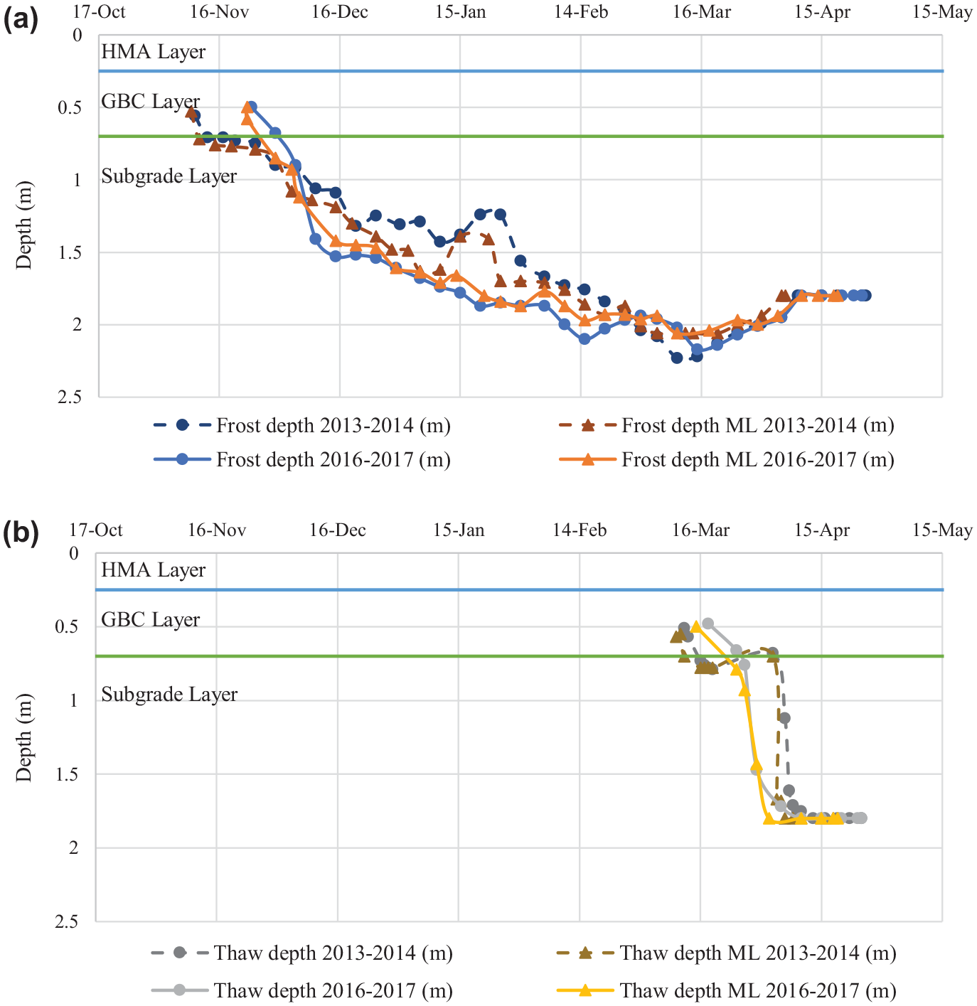
Measured and estimated (a) frost depths and (b) thaw depths from 2013 to 2014, and 2016 to 2017.

Figure 3a shows that the air temperature was above 0°C for a few days in January, February, and March 2014, but was not consistently above freezing. Therefore, the calculation of the thaw depth for 2014 and 2017 started in March. The predicted frost and thaw depths obtained from the Gaussian process regression ML model show good agreement with the measurement results, with the R² value being 0.93 for sixty frost depth samples and 0.91 for the sixteen thaw depth samples. The predicted trends align well with the measured trends.

Based on the pavement temperature recordings, in the period from 2013 to 2014, the frost reached the GBC layer on November 10, 2013 and reached the subgrade layer on November 28, 2013. Thawing began on March 12, 2014, and the frost and thaw depth are equal on April 6, 2014. Even though the temperature, at a depth of 1.80 m below the road surface, remained at 0°C until April 25, 2014, it did not affect the end date of the thawing process. Previous studies ( 16 , 18 ) have shown that once the frost and thaw depths meet, the freeze–thaw cycle is considered complete for that year. In the period from 2016 to 2017, the frost reached the GBC layer on November 24, 2016 and reached the subgrade layer on December 3, 2016. Thawing began on March 18, 2017, and the frost and thaw depths are equal on April 8, 2017.

According to the estimated results of the ML model, the frost started on November 9, 2013, and the frost depth reached the subgrade layer on November 27, 2013 as shown in Table 4. Thawing began on March 10, 2014, and the frost depth and thaw depth equal on April 10, 2014. For the winter from 2016 to 2017, the frost reached the base layer on November 23, 2016. Thawing began on March 15, 2017. Then, the frost and thaw depths are equal on April 5, 2017. The findings reveal a strong agreement between the ML model’s estimations and the measured values, with the differences typically within four days. The Gaussian process regression model demonstrates high accuracy not only for the years 2013–2014 and 2016–2017 but also for other years.

Table 4.

Comparison of Measured and Estimated Frost and Thaw Depths

Method	Frost reach granular base couree layer	Frost reach subgrade layer	Thawing start	Thawing end
2013–2014
Measurement	10 November	28 November	12 March	6 April
Machine learning	9 November	27 November	10 March	10 April
2016–2017
Measurement	24 November	3 December	18 March	8 April
Machine learning	23 November	30 November	15 March	5 April

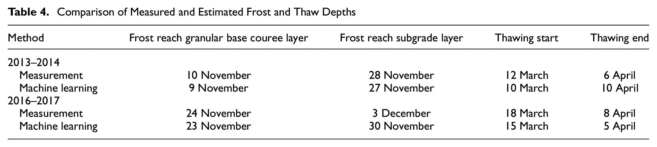
In the context of SLR and WWP policies, a four-day difference could influence the planning and decision-making processes. Therefore, it seems reasonable to incorporate a buffer or margin into the policy timelines to account for such variations in frost and thaw depth predictions. This adaptive approach ensures a more robust and resilient policy framework that can accommodate the inherent uncertainties in real-world conditions.

Comparing these results with information available from other studies mentioned above in the introduction section, we note that the proposed methodology, particularly leveraging ML models, presents a direct and accurate estimation of frost and thaw depths. Traditional methods often rely on indirect indices, leading to challenges in precision. The Gaussian process regression model, as demonstrated by the observed four-day difference, showcases improved accuracy and reliability in predicting critical dates for SLR and WWP. This distinction highlights the advancements it brings to the field and reinforces the practical applicability of ML in pavement management.

Moisture Content Variation of Base and Subgrade

Figure 5 illustrates the variation in moisture content during the same freeze–thaw period for the subgrade layers. The moisture content at the top of the subgrade layer started to drop on November 21, 2013 and November 26, 2016, respectively. The decrease in moisture content occurred approximately one week after the frost reached the subgrade layer. At a depth of 0.80 m, the moisture content started to increase on March 4, 2014. However, as shown in Figure 3a, the average daily air temperature dropped below 0°C again from March 20 to April 3, 2014. Consequently, the moisture content decreased from 0.34 to 0.22 m³/m³ on April 2, 2014. The moisture content at the depth of 1.8 m began to decrease on January 7, 2014 and December 12, 2016, respectively, following the changes in moisture content at shallower depths. Even though at a depth of 2.7 m the pavement temperature never dropped below 0°C, the moisture content at the same depth started to drop on January 12, 2014 and January 13, 2017. This reduction in moisture content below the frozen layer can be attributed to the migration of unfrozen water into the frozen layer ( 32 ).

Figure 5.

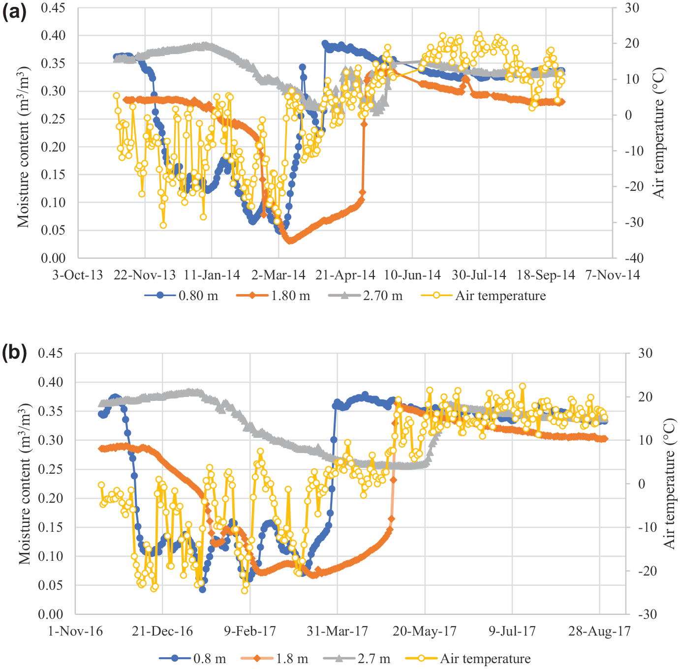
Average daily moisture content variation in the pavement structure from (a) 2013 to 2014; and (b) 2016 to 2017.

The moisture content collected by the TDR installed at a depth of 0.8 m was sensitive to temperature changes, resulting in sudden increases in January and February when the temperature rose. However, the moisture content collected at deeper locations only exhibited seasonal variation and did not increase with short-term temperature rises.

During the spring, the moisture content at a depth of 0.8 m was higher compared with other seasons, reaching its peak values for the entire year. Maximum values of 0.39 m³/m³ and 0.38 m³/m³ were observed on April 6, 2014 and April 16, 2017, respectively. According to the study by Asefzadeh et al. ( 12 ), the subgrade soil takes approximately 120 days to recover from the high-water level. Therefore, the subgrade soil would recover from the high-water level on August 6, 2014 and August 16, 2017, respectively.

In practical terms, the timing of soil moisture recovery should be considered when determining the end date of SLR and the initiation of WWP. Given that this study demonstrates a correlation between soil moisture content recovery and specific dates, incorporating this information into the policy framework can enhance its accuracy and effectiveness. To address this timing in the practice of SLR and WWP policies, we recommend adapting policy guidelines to align with the identified soil moisture recovery periods. Specifically, policy makers could utilize the recovery dates, such as August 6, 2014 and August 16, 2017, as key reference points for transitioning between load restrictions. This approach ensures a more dynamic and data-driven policy implementation, optimizing the balance between infrastructure protection and industry needs. Furthermore, incorporating such temporal considerations into policy frameworks reflects a forward-thinking approach, embracing the insights provided by the study.

Discussion

Actual Start and End Dates of WWP and SLR

Based on the theory proposed by Baïz et al. ( 16 ), the actual start and end dates of the SLR and WWP periods were determined based on the frost and thaw depths reaching specific thresholds and exhibiting continuous trends. The critical contact stress depth, which is the depth where the maximum traffic-induced vertical stress in the subgrade layer becomes less than 1% of the tire–pavement contact stress, was used to determine the start date of the WWP. According to previous research by Asefzadeh et al. ( 12 ), this critical depth is 1.05 m below the road surface in the IRRF test road. In alignment with the Alberta regulations, the WWP should start when the frost depth reaches 1.00 m ( 13 ). In this study, the WWP was considered to start when the frost depth reached a depth of 1.00 m below the road surface. Based on Alberta Transportation regulations, the WWP should end and the SLR should begin when the thaw depth reaches 0.25 m ( 33 ). The shallowest TDR was installed at a depth of 0.50 m below the road surface, so the SLR was considered to start and the WWP was considered to end when the thaw depth continuously exceeded 0 m (reaching the GBC layer). The SLR was considered to end when the frost depth and the thaw depth are equal, indicating the completion of the freeze–thaw cycle ( 18 ).

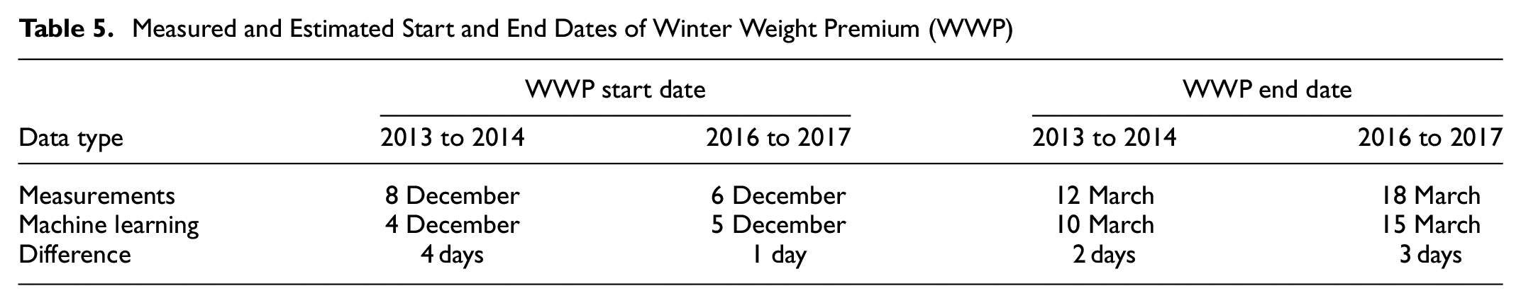
Table 5 presents the comparison of the actual start and end dates of the WWP between the winters of 2013 to 2014 and 2016 to 2017. Despite the winter of 2013 to 2014 being colder than the winter of 2016 to 2017, the WWP lasted longer in the winter of 2016 to 2017 (102 days) than in the winter of 2013 to 2014 (94 days). The WWP started on December 8, 2013 and ended on March 12, 2014, whereas it started on December 6, 2016 and ended on March 18, 2017. Table 6 demonstrates the measured and estimated start and end dates of the SLR. Although the monthly average air temperature in March 2014 was lower than that in March 2017, the SLR started six days earlier in 2014. The SLR started on March 12, 2014 and on March 18, 2017, and ended on April 6, 2014 and April 8, 2017. It lasted 25 days in the winter of 2013 to 2014 and 21 days in the winter of 2016 to 2017.

Table 5.

Measured and Estimated Start and End Dates of Winter Weight Premium (WWP)

	WWP start date		WWP end date
Data type	2013 to 2014	2016 to 2017	2013 to 2014	2016 to 2017
Measurements	8 December	6 December	12 March	18 March
Machine learning	4 December	5 December	10 March	15 March
Difference	4 days	1 day	2 days	3 days

Table 6.

Measured and Estimated Start and End Dates of Spring Load Restrictions (SLR)

	SLR start date		SLR end date
Data type	2013 to 2014	2016 to 2017	2013 to 2014	2016 to 2017
Measurements	12 March	18 March	6 April	8 April
Machine learning	10 March	15 March	10 April	5 April
Difference	2 days	3 days	4 days	3 days

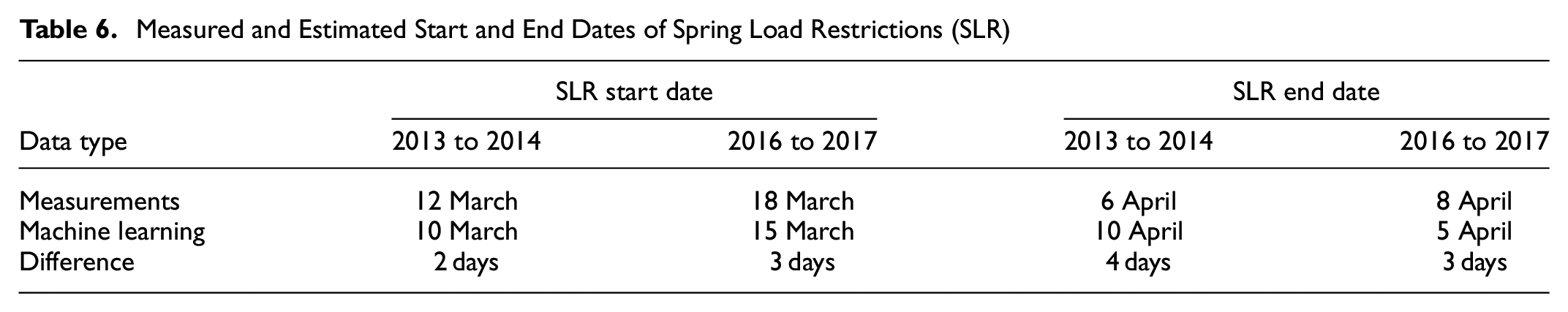
The differences between the measured and estimated results in both years were within four days. This demonstrates the high accuracy of the Gaussian process regression model, indicating that the ML model can be a practical method for determining the start and end dates of the WWP and SLR. Through the Gaussian process regression model, the estimated results indicate that the WWP lasted for 96 days from 2013 to 2014 and 100 days from 2016 to 2017. Additionally, the SLR was found to last for 31 days from 2013 to 2014 and 21 days from 2016 to 2017.

Observed Moisture Content at the Start and End of the Day for WWP and SLR

In this study, the moisture content at a depth of 0.80 m below the road surface was utilized to analyze the triggering and lifting of the SLR and WWP. This depth was chosen because the moisture content at this level exhibited a strong correlation with air temperature and was less influenced by other factors because of its distance from the road surface.

The observed moisture content at a depth of 0.80 m indicated the initiation of the WWP. In 2013, the moisture content started to decrease on November 21, 2013 and reached a value of 0.18 m³/m³ on December 8, 2013. Similarly, in 2016, the moisture content began to decrease on November 29, 2016 and dropped to 0.18 m³/m³ on December 6, 2016. The decrease in the soil moisture content corresponds to an increase in the soil resilient modulus ( 1 , 7 ), allowing for higher maximum axle loads on trucks. Therefore, the start date of the WWP aligned with the observed moisture content variation in the soil.

During the SLR period, the moisture content at a depth of 0.80 m showed an increasing trend. From March 12 to April 8, 2017, the moisture content increased from 0.07 to 0.37 m³/m³, with the highest value of 0.38 m³/m³ observed on April 16, 2017. A similar trend occurred in 2014, where the moisture content began to increase from 0.07 m³/m³ on March 9 and reached its highest value of 0.39 m³/m³ on April 6. Despite the frost depth and thaw depth meeting on April 6, 2014, the accumulated water in the soil could not drain from the subgrade layer. This is problematic because high soil moisture content combined with heavy truck traffic can lead to significant pavement damage ( 7 ).

Based on Alberta Transportation regulations, the thawing period should end around June 16 (with a possible variation of one week earlier or later) ( 33 ). On June 16, 2017, the moisture content was measured at 0.35 m³/m³. After 120 days from April 16, 2017, the moisture content decreased to 0.34 m³/m³ on August 17, 2017, which was selected as the moisture content base point. In 2014, the moisture content dropped to 0.34 m³/m³ on June 17, and in 2017 it dropped to the same value on June 25. It took 97 days in 2014 and 99 days in 2017 for the moisture content at a depth of 0.80 m to return to 0.34 m³/m³, indicating the discharge of accumulated water from the start date of the SLR. These observations indicate that frost and thawing depths can be utilized to estimate the start date of WWP and SLR. However, determining the end of the SLR should be based on a combination of frost and thaw depths along with the moisture content in the subgrade layer.

Limitations of the Machine Learning Models

The main limitation of the ML models used in this study, specifically the Gaussian process regression model, is their reliance on the training data and the consequent lack of generalizability of the data. In this case, the model was trained using pavement temperature data collected specifically from the IRRF test road. Therefore, its applicability to other road surfaces or geographical locations may be limited.

The accuracy and performance of ML models heavily depend on the quality, diversity, and representativeness of the training data. If the model is trained on a narrow or biased dataset, it may not capture the full range of variations and patterns present in different scenarios. This lack of generalizability can result in reduced accuracy and reliability when applied to new or unseen data.

To overcome this limitation, it would be beneficial to train the ML model using a larger and more diverse dataset that includes pavement temperature data from various locations and road types. This would enhance the model’s ability to generalize and provide accurate predictions in different contexts. Additionally, considering other relevant factors, such as the properties of pavement materials, the number of layers, and so on, could further improve the model’s performance and broaden its applicability.

Conclusion

The study utilized a ML model to predict the start and end dates of SLR and WWP by directly calculating the frost and thaw depths from the pavement temperature. Pavement temperatures collected from the IRRF test road from January 2013 to December 2020 were used to develop ML models. Air temperature, day of the year, and depth were used as the input parameters. The Gaussian process regression model performed the best with an R² of 0.99 and an RMSE of 1.45°C. Pavement temperatures collected from November 2013 to April 2014 and November 2016 to April 2017 were used to discuss the accuracy of the ML prediction. Furthermore, the study discussed some existing theories that proposed to determine the start and end dates of the WWP and SLR directly by frost and thaw depths. Moisture content is a dominant factor in the structural capacity of the soil. However, these existing theories did not consider the soil’s moisture content. This study used moisture content collected from the IRRF test road during the same period to discuss the validity of these existing theories. The following conclusions were drawn based on a detailed analysis of measured and estimated results, and moisture content variation.

The Gaussian process regression model demonstrated high accuracy in estimating frost and thaw depths (R² of 0.93 and 0.91 for the frost and thaw depths, respectively), making it a practical method for determining the start and end dates of WWP and SLR in pavement structures.

A comparison with measured results showed good agreement, with differences in start and end dates of WWP and SLR occurring within four days.

The soil moisture content at a depth of 0.80 m below the pavement exhibited significant changes corresponding to the start of WWP and SLR, validating the existing theories. However, when the frost depth and the thaw depth are equal, the accumulated moisture content in the subgrade layer could not effectively discharge, leading to prolonged high moisture content levels in the soil beyond the end date for SLR.

The subgrade layer required approximately 120 days to discharge excess water, but it actually took fewer days (97 days in 2014 and 99 days in 2017), which emphasized the need to consider soil moisture content when determining the end date of SLR.

One of the key objectives of this research is to emphasize the significance of incorporating soil moisture content variation into the determination of SLR and WWP start and end dates. We recognize the limitations of existing methods that overlook the influence of moisture content, and the findings underscore the importance of addressing this variable in pavement management. With regard to the enhanced integrated climatic model, our investigation revealed that its accuracy in predicting moisture content did not align with the specific requirements of the study, as indicated in the literature ( 27 ). Previous study ( 27 ) also highlights that ML emerges as a powerful alternative for predicting moisture content in base and subgrade layers.

As recommendations, we advocate for the integration of ML methods to capture the nuanced variations in soil moisture content. ML techniques, as demonstrated in the literature, have shown promise in providing accurate predictions and can be a valuable tool for pavement management departments. These points are emphasized in the manuscript to ensure clarity on our stance with regard to the role of moisture content in the determination of SLR and WWP.

In conclusion, the ML model could be a practical method to determine the start and end dates of the WWP and SLR; however, the excess water could not discharge when the frost depth and thaw depth are equal, and the high moisture content with truck transportation on the road may lead to serious damage to the pavement. Therefore, it is necessary to consider the soil moisture content when determining the end date of the SLR.

The model was developed using years of historical data, and it showed high accuracy in years of pavement temperature prediction. Thus, once the air temperature data are available, it should work for the pavement temperature prediction and frost and thaw depth estimation. However, once more historical data are available, it is necessary to improve the model by incorporating climate change projections. The ability of the proposed model to estimate the start date of WWP and SLR, particularly by considering moisture content variations, opens avenues for optimizing SLR. By proactively managing moisture content and frost and thawing depths, the duration of SLR could potentially be shortened, aligning with industry development goals. Shortening SLR not only supports industry operations but also contributes to pavement protection. Balancing the needs of industry development with the imperative of preserving pavement integrity is a key aspect of the methodology’s potential impact. It is noteworthy that although our findings support the idea that a data-driven approach could potentially shorten the duration of SLR, it is also plausible that such an approach could affect the duration of WWP. Recognizing this dual effect is crucial in understanding the broader implications of our methodology on industry practices and pavement integrity preservation.

Moreover, by incorporating many input parameters, such as the properties of pavement materials, the number of layers, and so on, the generalizability of the model could improve. However, such expansive data are not currently available. Although the generalizability of the machine learning model is limited and a dataset collected from the specific projects is necessary, ML models provide a robust option to improve road management.

Footnotes

Author Contributions

The authors confirm contribution to the paper as follows: study conception and design: A. Bayat, L. Hashemian; data collection: Y. Huang; analysis and interpretation of results: L. Hashemian, T. Baghaee Moghaddam, Y. Huang; draft manuscript preparation: L. Hashemian, T. Baghaee Moghaddam, Y. Huang. All authors reviewed the results and approved the final version of the manuscript.

Declaration of Conflicting Interests

The author(s) declared no potential conflicts of interest with respect to the research, authorship, and/or publication of this article.

Funding

The author(s) received the following financial support for the research, authorship, and/or publication of this article: The authors would like to thank Alberta Transportation, the Edmonton Waste Management Centre, the City of Edmonton, and Alberta Recycling for their financial and in-kind support of the Integrated Road Research Facility test road. Funding from the Natural Sciences and Engineering Research Council of Canada (NSERC) is gratefully acknowledged.

ORCID iD

Leila Hashemian

Data Accessibility Statement

Participants in this study did not give written consent to share their data publicly, therefore supporting data cannot be obtained because of the sensitivity of the study.

References

ARA, Inc., ERES Consultants Division. Guide for Mechanistic–Empirical Design of New and Rehabilitated Pavement Structures. Final Report, NCHRP Project 1-37A. Transportation Research Board of the National Academies, Washington, D.C., 2004. http://www.trb.org/mepdg/guide.htm.

Bohra

N. C.

Altschaeffl

A. G.

Drumm

E. C.

Reeves

J. S.

Madgett

M. R.

Trolinger

W. D.

Subgrade Resilient Modulus Correction for Saturation Effects. Journal of Geotechnical and Geoenvironmental Engineering, Vol. 125, No. 3, 1999, pp. 233–235. https://doi.org/10.1061/(asce)1090-0241(1999)125:3(233)

Christopher

B. R.

Schwartz

C. W.

Boudreaux

Berg

R. R.

Geotechnical Aspects of Pavements. Report No. FHWA-NHI-05-037. U. S. Federal Highway Administration, 2006.

Haghi

N. T.

Hashemian

Bayat

Effects of Seasonal Variation on the Load-Bearing Capacity of Pavements Composed of Insulation Layers. Transportation Research Record: Journal of the Transportation Research Board, 2016. 2579: 87–95.

Huang

Molavi Nojumi

Hashemian

Bayat

Performance Evaluation of Different Insulating Materials Using Field Temperature and Moisture Data. Transportation Research Record: Journal of the Transportation Research Board, 2021. 2675: 595–607. https://doi.org/10.1177/03611981211003572

Janoo

Shepherd

Seasonal Variation of Moisture and Subsurface Layer Moduli. Transportation Research Record: Journal of the Transportation Research Board, 2000. 1709: 98–107.

Haghi

S. N. T.

Use of Waste/Recycled Material as Insulation in Road Construction. Doctoral thesis. University of Alberta, Canada, 2019.

Bayat

Field and Numerical Investigation to Determine the Impact of Environmental and Wheel Loads on Flexible Pavement. Doctoral thesis. University of Waterloo, Canada, 2009.

Al-Qadi

I. L.

Wang

Yoo

P. J.

Dessouky

S. H.

Dynamic Analysis and in Situ Validation of Perpetual Pavement Response to Vehicular Loading. Transportation Research Record: Journal of the Transportation Research Board, 2008. 2087: 29–39. https://doi.org/10.3141/2087-04

10.

Shafiee

M. H.

Hashemian

Bayat

Seasonal Analysis of Flexible Pavement Response to Falling Weight Deflectometer. International Journal of Pavement Research and Technology, Vol. 8, No. 5, 2015, pp. 346–352. https://doi.org/10.6135/ijprt.org.tw/2015.8(5).346

11.

Canada Cartage Group of Companies. Canadian Spring Thaw Regulations (Updated). https://www.canadacartage.com/2021-canadian-spring-thaw-regulations/#:~:text=This%20will%20usually%20include%20limitations,frost%2C%20and%20road%20tolerance%20testing. Accessed June 8, 2023.

12.

Asefzadeh

Hashemian

Haghi

N. T.

Bayat

Evaluation of Spring Load Restrictions and Winter Weight Premium Duration Prediction Methods in Cold Regions According to Field Data. Canadian Journal of Civil Engineering, Vol. 43, No. 7, 2016, pp. 667–674. https://doi.org/10.1139/cjce-2015-0554

13.

Bradley

A. H.

Ahammed

M. A.

Hilderman

Kass

Responding to Climate Change With Rational Approaches for Managing Seasonal Weight Programs in Manitoba. In Cold Regions Engineering 2012: Sustainable Infrastructure Development in a Changing Cold Environment (Jon E. Zufelt, ed.), American Society of Civil Engineers, Reston, VA, 2012, pp. 391–401.

14.

Minnesota Department of Transportation. Policy and Process for Seasonal Load Limit Starting and Ending Date. No. 14-10-MAT-02 October 7. Minnesota Department of Transportation, Policy, Safety and Strategic Initiatives Division, Technical Memorandum, 2014.

15.

Mahoney

J. P.

Rutherford

M. S.

Hicks

R. G.

Guidelines for Spring Highway Use Restrictions. No. FHWA-TS-87-209. Washington State Department of Transportation, Olympia, WA, 1987.

16.

Baïz

Tighe

S. L.

Haas

C. T.

Mills

Perchanok

Development of Frost and Thaw Depth Predictors for Decision Making about Variable Load Restrictions. Transportation Research Record: Journal of the Transportation Research Board, 2008. 2053: 1–8. https://doi.org/10.3141/2053-01

17.

Bao

Liu

Bland

A Multivariate Freezing-Thawing Depth Prediction Model for Spring Load Restriction. Cold Regions Science and Technology, Vol. 167, 2019, p. 102856. https://doi.org/10.1016/j.coldregions.2019.102856

18.

Bao

Azmoon

(Leo) Liu

Freeze-Thaw Depth Prediction With Constrained Optimization for Spring Load Restriction. Transportation Geotechnics, Vol. 26, 2021, p. 100419. https://doi.org/10.1016/j.trgeo.2020.100419

19.

Liu

Sun

Temperature Predictions for Asphalt Pavement With Thick Asphalt Layer. Construction and Building Materials, Vol. 160, 2018, pp. 802–809.

20.

Tabrizi

S. E.

Xiao

Thé

J. V. G.

Saad

Farghaly

Yang

S. X.

Gharabaghi

Hourly Road Pavement Surface Temperature Forecasting Using Deep Learning Models. Journal of Hydrology, Vol. 603, 2021, p. 126877.

21.

Chen

Wang

Xie

Pavement Temperature Prediction: Theoretical Models and Critical Affecting Factors. Applied Thermal Engineering, Vol. 158, 2019, p. 113755. https://doi.org/10.1016/j.applthermaleng.2019.113755

22.

Milad

A. A.

Adwan

Majeed

S. A.

Memon

Z. A.

Bilema

Omar

H. A.

Abdolrasol

M. G. M.

Usman

Yusoff

N. I. M.

Development of a Hybrid Machine Learning Model for Asphalt Pavement Temperature Prediction. IEEE Access, Vol. 9, 2021, pp. 158041–158056. https://doi.org/10.1109/ACCESS.2021.3129979

23.

Huang

Molavi Nojumi

Hashemian

Bayat

Evaluation of a Machine Learning Approach for Temperature Prediction in Pavement Base and Subgrade Layers in Alberta, Canada. Journal of Transportation Engineering, Part B: Pavements, Vol. 149, No. 1, 2023, p. 04022076. https://doi.org/10.1061/JPEODX.PVENG-1010

24.

Molavi Nojumi

Huang

Hashemian

Bayat

Application of Machine Learning for Temperature Prediction in a Test Road in Alberta. International Journal of Pavement Research and Technology, Vol. 15, No. 2, 2022, pp. 303–319. https://doi.org/10.1007/s42947-021-00023-3

25.

Huang

Molavi Nojumi

Ansari

Hashemian

Bayat

Evaluation of Machine Learning Approach for Base and Subgrade Layer Temperature Prediction at Various Depths in the Presence of Insulation Layers. International Journal of Pavement Engineering, Vol. 24, No. 1, 2023, p. 2180640. https://doi.org/10.1080/10298436.2023.2180640

26.

Abo-Hashema

M. A.

Modeling Pavement Temperature Prediction Using Artificial Neural Networks. In Airfield and Highway Pavement 2013: Sustainable and Efficient Pavements (I. L. Al-Qadi and S. Murrell, ed.), American Society of Civil Engineers, Reston, VA, 2013, pp. 490–505.

27.

Milad

Adwan

Majeed

S. A.

Yusoff

N. I. M.

Al-Ansari

Yaseen

Z. M.

Emerging Technologies of Deep Learning Models Development for Pavement Temperature Prediction. IEEE Access, Vol. 9, 2021, pp. 23840–23849.

28.

Huang

Molavi Nojumi

Ansari

Hashemian

Bayat

Evaluating the Use of Machine Learning for Moisture Content Prediction in Base and Subgrade Layers. Road Materials and Pavement Design, Vol. 24, 2023, pp. 2910–2928. https://doi.org/10.1080/14680629.2023.2182135

29.

Topp

G. C.

Davis

J. L.

Annan

A. P.

Electromagnetic Determination of Soil Water Content: Measurements in Coaxial Transmission Lines. Water Resources Research, Vol. 16, No. 3, 1980, pp. 574–582.

30.

Bonaccorso

. Machine Learning Algorithms: Popular Algorithms for Data Science and Machine Learning. Packt Publishing Ltd, Birmingham, UK, 2018.

31.

Schulz

Speekenbrink

Krause

A Tutorial on Gaussian Process Regression: Modelling, Exploring, and Exploiting Functions. Journal of Mathematical Psychology, Vol. 85, 2018, pp. 1–16. https://doi.org/10.1016/j.jmp.2018.03.001

32.

Hoekstra

Moisture Movement to a Freezing Front. Symp on Geochem, Precipitation, Evaporation, Soil Moisture, Hydom, Proc Gen Assembly of Bern, 1967, pp. 411–417.

33.

2023 Government of Alberta. Road Restrictions and Bans – Overview. https://www.alberta.ca/road-restrictions-and-bans-overview.aspx#jumplinks-2%20%20%20https://journals.sagepub.com/doi/10.3141/1989-67. Accessed June 8, 2023.

Application of the Machine Learning Method to Determine Spring Load Limits and Winter Weight Premium

Abstract

Keywords

Machine Learning Model Development

Data Characteristics

Model Development

Air Temperature

Comparison of Measured and Estimated Frost and Thawing Depths

Moisture Content Variation of Base and Subgrade

Discussion

Actual Start and End Dates of WWP and SLR

Observed Moisture Content at the Start and End of the Day for WWP and SLR

Limitations of the Machine Learning Models

Conclusion

Footnotes

Author Contributions

Declaration of Conflicting Interests

Funding

ORCID iD

Data Accessibility Statement

References