Sage Journals: Discover world-class research

Abstract

Urban arterials near freeway interchanges are vital components of urban road infrastructure, connecting high-mobility freeway networks to the more accessible but lower-mobility urban network. In this study, the operational safety of these arterials is examined and the relationship between roadway geometry and safety performance is investigated. To assess operational safety, lane changes were considered as a risk factor, and the number of lane changes in each study subsegment was recorded. Segments were categorized as upstream or downstream based on their location relative to the intersection. The number of lane changes served as a safety performance measure, and was analyzed using linear regression models. The results indicate that downstream segments experienced decreased safety performance when median storages were present, while adding right running bays improved safety. Median openings and increased numbers of driveways negatively affected safety in these segments. For upstream segments, right turning bays were found to impair safety performance the most, followed by the number of driveways. The closer the driveways were to the interchange; the worse was the effect on the safety performance. In summary, this research highlights the importance of geometric design elements when considering the safety performance of urban arterials. It is crucial to consider geometric design elements, such as median storages, driveways, and other elements, as a part of a larger system rather than isolated elements, so as to provide safer arterials near freeway interchanges.

Keywords

infrastructure roadway design performance effects of geometric design interchanges and freeways geometric design intersections geometric design operations access control arterials safety modeling and forecasting

Urban roads in the U.S. constitute approximately 25% of the total road network but account for about two-thirds of vehicle miles traveled (VMT) ( 1 – 3 ). The expected growth in VMT in the coming years underscores the need for optimal management of transportation networks, considering the limited potential for physical infrastructure expansion ( 4 ). Interchanges where freeway and urban networks intersect are of particular importance, as they facilitate the transition between different driving environments and accommodate various types of demand and a high density of commercial land uses.

Interchanges where freeway networks meet urban networks are important, as they facilitate the transition between two different driving environments, are host to many commercial land uses, and service different demand types. Transportation designers and planners face several questions when designing interchanges. How far should the interchange be placed from the signalized intersections? How far from the interchange should the first access point be? How many access points should a shopping plaza have? Should right turns at the terminal intersection be stop- or yield-controlled? In this study diverse data sources were utilized and simulation techniques were employed to build a comprehensive database encompassing various design options. The database was analyzed to evaluate the relationship between design choices and the safety performance of selected study locations. Two models were developed to analyze these relationships and provide recommendations for optimal design options.

Previous research has been extensively conducted to examine various elements of roadway design, often focusing on economic evaluations based on such factors as injuries, fatalities, and other losses. These studies have explored various elements including the number of lanes ( 5 , 6 ), lane width ( 6 ), surface type ( 7 ), cross slope ( 8 ), and surface friction ( 9 ). Cribbins et al. ( 10 ) evaluated median width, while Foley ( 11 ) investigated the frequency of median openings and the type of median barrier. Auxiliary lanes, such as left turn lanes and transition lanes (for speed adjustment), as well as shoulder and roadside characteristics, vertical alignment, and traffic control devices have also received much attention. Avelar et al. ( 12 ) categorized parameters that influenced arterial highway safety into the following seven categories, namely driveway spacing, proximity to interchange and intersection, traffic signal control, driveway type, roadway characteristics, land use, and median type. They concluded that segment length, average annual daily traffic, median type (two way left turn lane [TWLTL]), and having four lanes on the rural highway were the most significant factors, contributing to the most crashes.

Simulation techniques have played a prominent role in transportation research. Simulation models are constructed by generating vehicles, assigning routes ( 13 – 16 ), determining driver behaviors (including lane change preferences) ( 17 – 20 ), and modifying infrastructural and environmental properties. Stochastic processes are used to generate random numbers, which are then employed in constructing simulation models. As different random seeds yield different numbers, several iterations are usually run with various random seeds to ensure consistent and reliable results. Determining the most appropriate number of simulation runs helps to reach reliable results while avoiding unnecessary resource expenditure (in relation to time and processing) ( 21 ). There are two major approaches to determining the number of simulation runs necessary ( 22 , 23 ): one involves calculating means, standard deviations, and confidence intervals to derive the required number of simulation runs, while the other incrementally increases the number of runs based on calculated means, standard deviations, and desired margins of error. In this study, the confidence interval method (the first method) was employed, along with engineering judgment, to determine the final number of simulation runs:

n = ⌈ \frac{S D^{2} t_{c}^{2}}{ϵ^{2}} ⌉

(1)

In Equation 1, the symbol ⌈⌉ represents the ceiling function, which rounds up to the nearest integer value. The symbol ε represents the allowable percentage error of the estimate. SD refers to the sample standard deviation, and $t_{c}$ represents the critical value for the t distribution, based on the desired confidence interval.

The simulation runs were treated as samples, with the aim of determining the appropriate number of runs. Several simulation runs were conducted and the model outputs were used to calculate a new minimum number of required runs. Since the models consistently produced stable outputs, the calculated required number of runs was small (smaller than four). However, to ensure robustness, additional iterations were included, and the simulation was ultimately run 10 times. Each simulation run represented one hour of real-world conditions.

To validate the number of lane changes obtained from the simulation, the data from video files were taken as the ground truth value (µ0). A confidence interval test was conducted to determine whether the µ0 value fell within the 99% confidence interval of the simulation results. The validation process is explained in detail in the dissertation published by Shirinzad ( 24 ).

Employing a confidence interval approach, a margin of error was calculated for the simulation outputs. The real-world measurements were then examined to determine whether they fell within the confidence interval for each segment. This comparison helped validate the accuracy and reliability of the simulation results.

Methods

The data utilized in this research were obtained from the NCHRP 07-23 project simulation models ( 25 ). The initial data for the NCHRP 07-23 report were collected through various means, including video recording and the use of a GPS-enabled pilot vehicle to gather travel time data. Such information as volumes, origin–destination matrices, lane change data, and signal timing were extracted from the video files. These data sets were employed to develop, calibrate, and validate simulation models.

For this study, three locations near diamond interchanges were selected as the study sites. Diamond interchanges are commonly found in the U.S. and consist of four one-way ramps forming a diamond shape, connecting an urban arterial road to a crossing freeway. Each study site encompassed four intersections, comprising two terminal intersections at the interchange and two adjacent signalized intersections, one at each side of the interchange. Figure 1 is a diagram of the models. The study sites were divided into four study segments, labeled 1 to 4 in Figure 1.

Figure 1.

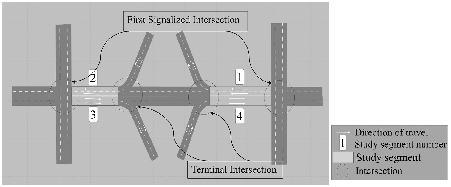
General setup of simulation model.

Once the simulation models were constructed, four key variables were selected for manipulation, to create different scenarios. These variables were volume, driveway settings, median option, and right turning movement control type at the terminal intersection. Table 1 summarizes the options utilized to develop the simulation models, with the option names presented within parentheses.

Table 1.

Scenario Options for Simulation Models

Volume	Driveway	Median	Right turn control
Off-peak (MV0)	No change (DW0)	No change (MED0)	Stop (OP0)
Peak (MV1)	One driveway (DW1)	Raised (MED1)	Yield (OP1)
0.5C (MV2)	No driveways (DW2)	na*	na*
0.75C (MV3)	na*	na*	na*
Capacity (MV4)	na*	na*	na*

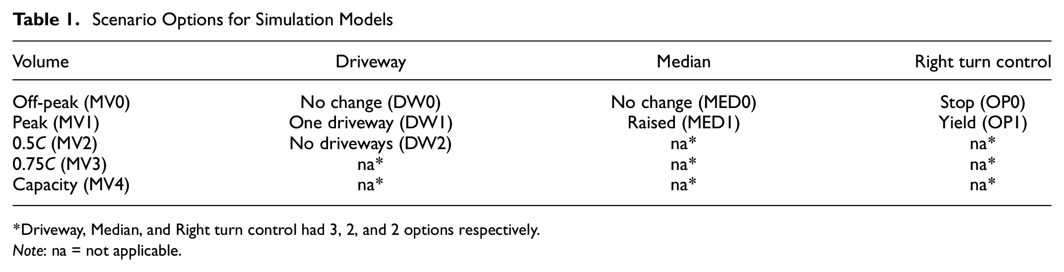
Driveway, Median, and Right turn control had 3, 2, and 2 options respectively.Note: na = not applicable.

A full factorial study was conducted, in which all available options for each variable were combined with all other variable options to create different scenarios. To facilitate this process, a Python code was developed to create scenarios and prompt VISSIM simulation software to run them. Several output files were collected for this study, including the following.

Vehicle records output file. This file logged information about each vehicle at specified intervals. The recorded data, which could be adjusted based on research requirements, included vehicle number (ID), simulation run number, origin zone, destination zone, lane changes, and delay. One vehicle records file was generated for each simulation run. For instance, if a site had 60 scenarios and 10 runs for each scenario, a total of 600 files were created. Each file contained data for all four study segments, resulting in 240 study segments within the network.

Lane change data file. This file captured information about each lane change movement, including the vehicle number, link number, lane number, speed, acceleration, and details about leading and lagging vehicles. A code written in R was utilized to extract the necessary data for each lane change movement from the vehicle records output file. Like the vehicle records file, a lane change data file was generated for each simulation run. In the case of a study segment with 60 scenarios and 10 runs per scenario, 600 lane change data files were created.

Data collection points. These points were positioned immediately after each stop line at every intersection to record the number of vehicles passing that point during each simulation run.

In addition to the VISSIM output data, Google Maps was used to measure geometric characteristics for inclusion in the analysis. Volumes were collected for off-peak and peak periods from the videos. Other volume options included in the study were the 50% capacity, 75% capacity, and full capacity values. Peak and off-peak volumes were obtained directly from the study site videos. Segment capacities were calculated based on the 2016 Highway Capacity Manual ( 26 ) and were distributed according to peak conditions among main origins and destinations to match the capacity conditions. The 50% capacity and 75% capacity volumes were then derived from the capacity origin–destination volumes. Figure 2 illustrates the collected variables for each study segment.

Figure 2.

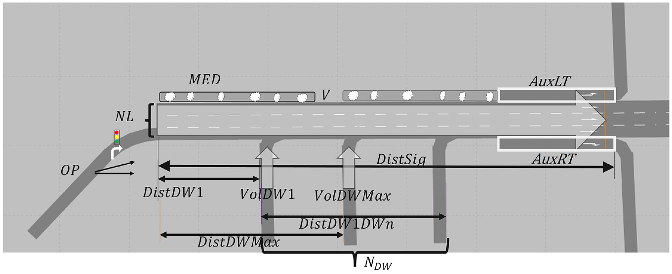
Collected design and operation variables for study segments.Note: Expansions/definitions of teems used in the figure: MED = Median; V = Volume, AuxLT = Auxiliary Left Turn lane; NL = Number of Lanes; OP = Operation Option (right turn option); DistDW1 = Distance of the first Driveway to upstream intersection; VolDW1 = Volume of the first Driveway; VolDWMax = Volume of the Driveway with Maximum volume; DistSig = Distance between two Signalized intersections; AuxRT = Auxiliary Right Turn lane; DistDW1DWn = Distance of the first Driveway to the last Driveway; DistDWMax = Distance of the Driveway with Maximum volume from the upstream intersection; N_DW = Number of Driveways.

Following previous studies, surrogate safety measures were utilized instead of relying solely on crash statistics. In this case, the number of lane changes was chosen as a measure of risk. While measuring the exact number of lane changes can be challenging, the extensive data collected for this study facilitated the construction of precise simulation models capable of outputting the number of lane changes.

To validate the accuracy of the number of lane changes, the base condition simulation models were initially used. The validation process has been explained in more detail in the student report published by Dastgiri and Dixon ( 27 ), who subsequently developed various scenarios to account for different volumes, driveway settings, median openings, and right turning movements at the terminal intersection conditions.

Once the simulation models had been executed, the number and location of lane changes at each study segment were recorded. Each study segment was then divided into smaller subsegments. It was decided to divide each segment into five subsegments of equal lengths. This approach allowed for subsegment lengths to be proportionate to the corresponding segment lengths (ranging between 430 and 1310 ft), while ensuring that the subsegment lengths remained within a reasonable range.

In the regression analysis, a total of 30 independent variables were utilized. Here are the names and definitions of the independent variables.

AuxLt. Binary variable indicating the presence (1) or absence (0) of an auxiliary left-turning lane (no unit)

AuxRt. Binary variable indicating the presence (1) or absence (0) of an auxiliary right turning lane (no unit)

DenDw. Density of driveways measured (driveway/mi)

DistDw1. Distance from the upstream intersection to the first driveway (ft)

DistDw1DwN. Distance from the first driveway to the last driveway (ft)

DistSig. Distance from the upstream intersection to the first signalized intersection (ft)

DistUPSDwmax. Distance from the upstream intersection to the driveway with the largest volume (ft)

DistUPSLTLane. Distance from the upstream intersection to the beginning of the left-turning lane; if no left-turning auxiliary exists, this is equal to DistSig (ft)

DistUPSMed. Distance from the upstream intersection to the beginning of the first median opening (ft)

DistUPSRT. Distance from the upstream intersection to the beginning of the right turning lane (ft)

DistUPST1LT. Distance between the upstream intersection and the first point where cars can turn left; this can be a median opening or at the intersection, whichever is shorter (ft)

LenMedStor. Length of median storage (ft)

MdensDw. Modified density of driveways calculated as the number of driveways multiplied by 5280 (to convert to driveway/mi) and divided by the distance from the start of the first driveway to the end of the last driveway (driveway/mi)

MedContin. Binary variable indicating whether the median is continuous through the entire segment (1) or not (0) (no unit)

NL. Number of lanes (count)

NLC. Number of lane changes (count)

NoDw. Number of driveways (count)

NoLTLanes. Number of exclusive left-turning lanes (count)

NoMed. Number of median openings (count)

NoRTLanes. Number of exclusive right turning lanes (count)

SimVolLT. Simulated left-turning volume passed through the downstream intersection (vehicles per hour [vph])

SimVolRT. Simulated right turning volume passed through the downstream intersection (vph)

SimVolTru. Simulated through volume passed through the downstream intersection (vph)

SimVolUT. Simulated U-turn volume passed through the upstream intersection (vph)

TMed. Median type (1, raised median; 2, raised median with median opening; 3, TWLTL) (categorical)

TT. Travel time (s)

VolDwmax. Volume of largest volume driveway (vph)

WidthDw1. Width of first driveway (ft)

WidthDwMax. Width of the driveway with the largest volume (ft)

WiMedOp. Length of the median opening (ft)

As mentioned before, to model the distribution of lane changes on the segments, each study segment was divided into five equal subsegments. The number of lane changes was measured on each subsegment. The coefficient of variation (CV), calculated as the ratio of the standard deviation to the mean, is a statistical measure of fluctuation. Since CV is typically a small number between 0 and 1, the authors used 100 × CV (referred to as the flux in this study) as the measure of fluctuation in the number of lane changes on study segments. The flux was employed as the dependent variable, while the collected design variables were used to construct statistical models.

Results

The main objective of this research was to examine the influence of design factors on operational safety in the vicinity of interchanges on urban arterials. To achieve this goal, a safety performance measure was devised to determine the variation in the number of lane changes occurring on a segment of urban arterial. The underlying hypothesis was that lane change maneuvers would have a negative effect on the safety performance of traffic on urban arterials near diamond interchanges. Furthermore, it was postulated that when lane changes occurred close to each other the cumulative risk of an incident would significantly increase.

Preliminary analysis revealed that dividing the study segments into upstream and downstream sections improved the accuracy of the statistical model. Consequently, two models were constructed to establish the relationship between the safety performance measure (flux) and the design variables.

As mentioned earlier, three specific sites were selected for this study, with 60 scenarios built for sites 1 and 3, and 30 scenarios built for site 2. By combining these scenarios, a comprehensive database consisting of 6,000 data points was compiled. Figure 3 is the probability density plot depicting the distribution of CV, which serves as an indicator of the fluctuation in lane change frequency.

Figure 3.

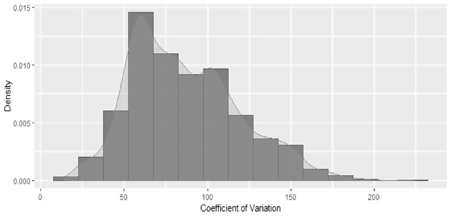
Density plot of coefficient of variation for all segments.

Figure 4 shows histograms based on the segment characteristics. Segments 1 and 3 were located upstream of the terminal intersections, while segments 2 and 4 were located downstream of the terminal intersections.

Figure 4.

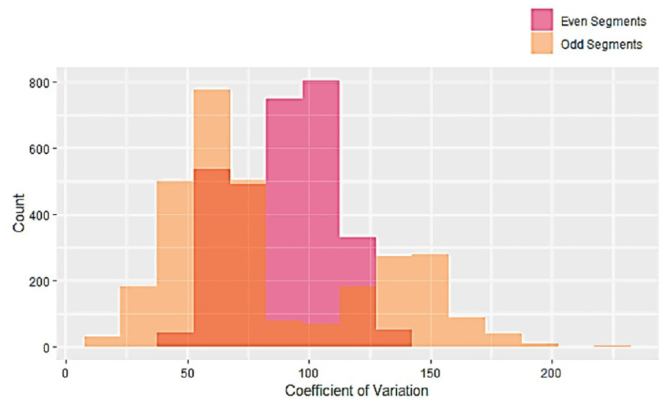
Histograms of coefficient of variation for even and odd segments.

The main data set was divided based on scenario variables and then paired t tests were conducted to identify whether changing an option affected the number of lane changes. Paired t tests were used because the numbers of lane changes were distributed differently along each segment and it was important to pair the distributions based on the segments. The number of lane changes were compared in one subsegment by keeping all but one variable constant.

Table 2 shows the results of all paired t tests. In all comparisons (each row) the null hypothesis (H0) was that the mean of the difference (µd) between the two sets was equal to zero. The alternative hypothesis (H1) was that µd was not equal to zero.

Table 2.

Paired t Test Results

Set 1	Set 2	t	p	Mean of the differences
MV0	MV1	−61.18	<2.2 × 10⁻¹⁶	−26.78
MV0	MV2	−52.96	<2.2 × 10⁻¹⁶	−83.365
MV0	MV3	−30.02	<2.2 × 10⁻¹⁶	−41.68
MV0	MV4	−26.66	<2.2 × 10⁻¹⁶	−59.80
MV1	MV2	−43.48	<2.2 × 10⁻¹⁶	−56.58
MV1	MV3	−11.16	<2.2 × 10⁻¹⁶	−14.89
MV1	MV4	−14.90	<2.2 × 10⁻¹⁶	−33.01
MV2	MV3	26.12	<2.2 × 10⁻¹⁶	41.68
MV2	MV4	9.82	<2.2 × 10⁻¹⁶	23.56
MV3	MV4	−14.32	<2.2 × 10⁻¹⁶	−18.12
DW0	DW1	1.79	0.073	0.65
DW0	DW2	−0.159	0.87	−0.07
DW1	DW2	−1.74	0.082	−0.72
MED0	MED1	46.34	2.2 × 10⁻¹⁶	47.50
OP0	OP1	−0.83	0.41	−0.06

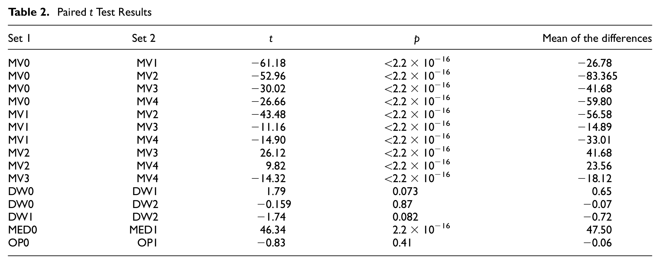
The results show that volume and median options had a significant effect on the distribution of lane changes on study subsegments, while different driveway and operation options did not influence the number of lane changes in the study subsegments. Since the values of p for different driveways were only slightly over the criterion of 0.05, it was decided to include these variables in the final statistical analysis models and investigate their effect.

Next, a regression model was built to investigate the effect of design variables on the study performance measure. Lasso regression was used to conduct the regression analysis. Choosing the shrinkage penalty parameter (lambda) in the final model affected the model’s coefficients. Figure 5 shows R² scores for the models made, with a range of 100 lambda values. The lambda value producing the lowest cross-validation error was chosen as the best lambda value, but the model with the lowest cross-validation error included a larger number of independent variables (forced fewer coefficients to be exactly zero).

Figure 5.

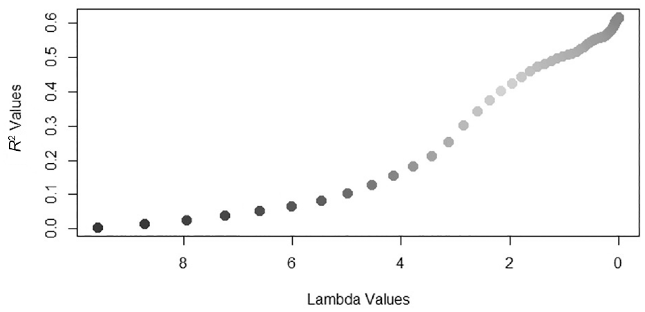
R² scores for different lambda values.

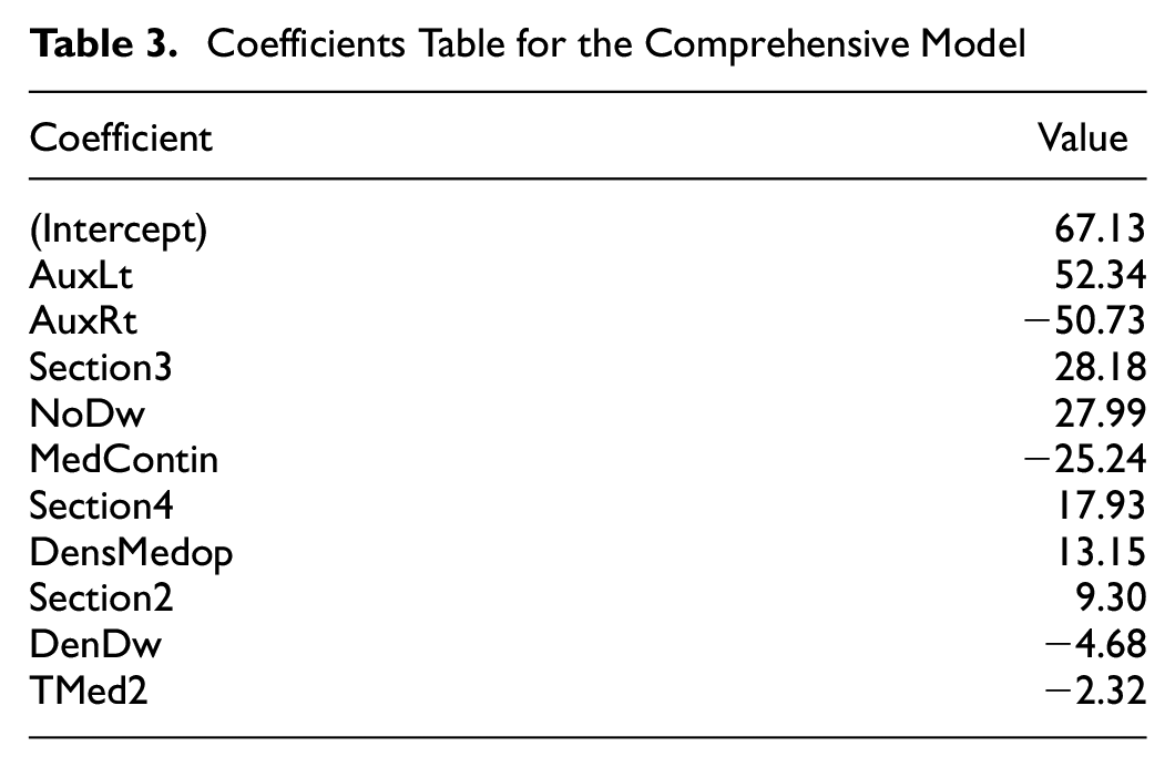
Table 3 shows the 10 largest coefficients for the best lambda, sorted from largest to smallest. The R² score for this model was 0.61; it can be seen that the binary variables for Section3 and Section2 were among the independent variables with the largest coefficients.

Table 3.

Coefficients Table for the Comprehensive Model

Coefficient	Value
(Intercept)	67.13
AuxLt	52.34
AuxRt	−50.73
Section3	28.18
NoDw	27.99
MedContin	−25.24
Section4	17.93
DensMedop	13.15
Section2	9.30
DenDw	−4.68
TMed2	−2.32

Segments 1 and 3 were located upstream of freeway on-ramps (upstream segments) and segments 2 and 4 were located downstream of freeway off-ramps (downstream segments). For upstream segments, Table 4 summarizes the coefficient values. The R² score for this model was 0.75.

Table 4.

Coefficients Table for Upstream Segments

Coefficient	Value
(Intercept)	53.63
AuxRt	27.70
NoDw	14.60
Mden.Den	1.73
OP1	1.40
DenDw	1.00
VolDwmax	0.88
WidthDwMax	−0.80
NLCmeans	−0.64
MedContin	−0.41
MED1	−0.38

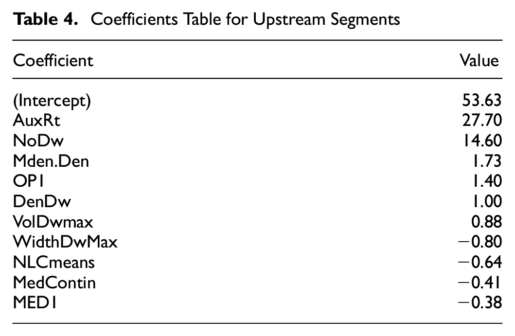
Table 5 summarizes the coefficient values for downstream segments. The R² score for this model was 0.71.

Table 5.

Coefficients Table for Downstream Segments

Coefficient	Value
(Intercept)	88.36
MedStor	37.20
AuxRt	−29.90
TMed2	4.77
NoDw	3.29
DW1	1.17
OP1	−0.69
DW2	0.44
DenDw	−0.44
VolDwmax	−0.27
WidthDw1	−0.19

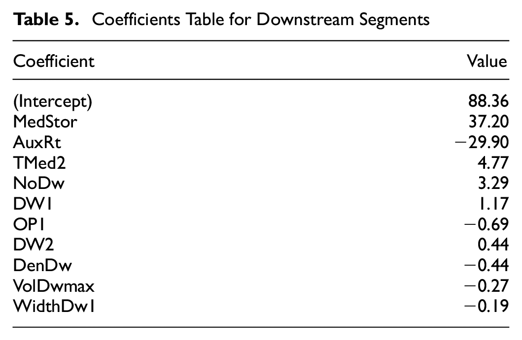
Comparison of R² scores between the comprehensive model, upstream model, and downstream model indicated that dividing the study segments into upstream and downstream categories significantly improved the fitness of the final models. This finding is intuitive, as the travel patterns in these two groups of segments differ. In the downstream segments, vehicles exiting the ramp and entering the downstream segments typically need to make more lane changes, with a significant portion of them making left turns at the first signalized intersection. Conversely, vehicles on the upstream segments are not as strongly affected by mandatory lane changes.

Following the division of the comprehensive dataset into upstream and downstream groups, two regression models were constructed. The proposed models for predicting flux in urban arterials near interchanges can be represented as

{flux}_{(down)} = 88.36 + 37.20 \times MedStor - 29.90 \times AuxRt + 4.77 \times Tmed 2 + 3.29 \times NoDW

(2)

{flux}_{(up)} = 55.63 + 27.70 \times AuxRt + 14.60 \times NoDw + 1.73 Mden / Den

(3)

The results of the regression models indicate that certain design factors had a notable effect on the fluctuation of lane changes in both upstream and downstream segments near interchanges.

For downstream segments, the provision of an auxiliary right turning lane or turning bay proved beneficial in reducing fluctuation. However, on upstream segments, the same design elements contributed to an increase in fluctuation. This suggests that this design feature has differential effects, depending on the location within the arterial segment; this could be because auxiliary right turn lanes or right turn bays on the upstream segments feed into the freeways and lane change maneuvers might take place as soon as an opportunity is provided, which might push right turning maneuvers into a specific subsegment, thus negatively affecting the flux.

The number of driveways had a significant influence on fluctuation, particularly on downstream segments, with a much higher coefficient (14.60) than for upstream segments (3.29). This implies that an increased number of driveways led to a larger fluctuation in the number of lane changes on downstream segments.

Among the design factors, the length of median storage had the highest coefficient for downstream segments, indicating that providing median storage contributed to increased fluctuation at these locations.

Furthermore, Type 2 medians (raised with openings) were found to increase fluctuation in the number of lane changes on downstream segments, while their effect on fluctuation in upstream segments was not statistically significant.

Overall, these findings highlight the importance of considering specific design factors, such as auxiliary lanes, driveways, median storage, and median type, to mitigate or manage the fluctuation of lane changes and enhance the operational safety of urban arterials near interchanges.

Discussion and Conclusions

This research was focused on examining the effect of design elements on safety performance in urban arterials near freeway interchanges. Three study sites near diamond interchanges were selected, and each study site consisted of four segments. A full factorial simulation was conducted, resulting in 600 scenarios, each of which was simulated 10 times using PTV-VISSIM (Planung Transport Verkehr-Verkehr In Stadten-SIMulationsmodell (German for “Planning Transportation Traffic- Traffic In Cities- Simulation Model”).

A safety performance measure was defined, and two statistical models were developed to analyze the fluctuation in the number of lane changes in upstream and downstream segments of urban arterials adjacent to diamond interchanges. The findings reveal that, in upstream segments, the presence of a right turning lane or turning bay led to an increase in the fluctuation of the number of lane changes. This indicates that when a right turning lane was present, lane change maneuvers tended to accumulate in a specific subsegment of the road. Additionally, the number of driveways had a significant effect on the fluctuation. For every additional driveway, the flux increased by a factor of 14.6. This suggests that reducing the number of access points could enhance safety in upstream segments of urban arterials.

In contrast, for downstream segments, providing right turning bays resulted in a decrease in flux, indicating that the presence of a right turning lane could improve the safety performance of traffic flow on urban arterials downstream from the terminal intersection.

The variable with the largest coefficient for downstream segments was whether there was median storage or not. This implies that raised medians with median openings that provide storage space had a negative effect on the safety performance of urban arterials downstream from the terminal intersection.

The results suggest that if there is a need to provide access to the opposing side of a road, it would be appropriate to investigate and assess the effects of other methods of providing access.

Overall, these findings provide insights into the design factors that can influence the safety performance of urban arterials near diamond interchanges, highlighting the importance of careful consideration and optimization of design elements to enhance traffic safety.

Footnotes

Authors’ Note

The data were produced using three of the simulation models that were developed under NCHRP project 07-23.

Author Contributions

The authors confirm contribution to the paper as follows: study conception and design: Karen Dixon, Maryam Shirinzad; data collection: Maryam Shirinzad, Karen Dixon; analysis and interpretation of results: Maryam Shirinzad, Karen Dixon; draft manuscript preparation: Maryam Shirinzad, Karen Dixon. All authors reviewed the results and approved the final version of the manuscript.

Declaration of Conflicting Interests

The author(s) declared no potential conflicts of interest with respect to the research, authorship, and/or publication of this article.

Funding

The author(s) disclosed receipt of the following financial support for the research, authorship, and/or publication of this article: This project was funded by the Safety through Disruption (Safe-D) National UTC, a grant from the U.S. Department of Transportation’s University Transportation Centers Program (federal grant number: 69A3551747115).

ORCID iDs

Maryam Shirinzad

Karen Dixon

References

FHWA and FTA. Conditions and Performance Report. U.S. Department of Transportation, Washington, D.C., 2006.

FHWA and FTA. Conditions and Performance Report. U.S. Department of Transportation, Washington, D.C., 2015, p. 544.

FHWA and FTA. Conditions and Performance Report. U.S. Department of Transportation, Washington, D.C., 2010.

Board

T. R.

Special Report 260, Strategic Highway Research Program. Transportation Research Board, The National Academies, Washington, D.C., 2001.

Shaw

Performance Measures of Operational Effectiveness for Highway Segments and Systems. Transportation Research Board, Washington, D.C., 2003.

Zegeer

C. V.

Deen

R. C.

Mayes

J. G.

The Effect of Lane and Shoulder Widths on Accident Reductions on Rural, Two-Lane Roads. Transportation Research Board, Washington, D.C., 1980.

Heimbach

C. L.

Hunter

W. W.

Chao

G. C.

Paved Highway Shoulders and Accident Experience. Journal of Transportation Engineering, Vol. 100, No. 4, 1974, pp. 889–907.

Dart

O. K.

Mann

Relationship of Rural Highway Geometry to Accident Rates in Louisiana. Highway Research Record, Vol. 312, 1970, pp. 1–16.

McCullough

B. F.

Hankins

K. D.

Skid Resistance Guidelines for Surface Improvements on Texas Highways. Highway Research Record, Vol. 131, 1966, pp. 204–217.

10.

Cribbins

P. D.

Horn

J. W.

Beeson

F. V.

Taylor

R. D.

Median Openings on Divided Highways: Their Effect on Accident Rates and Level of Service. Highway Research Record, Vol. 188, 1967, pp. 140–157.

11.

Foley

J. L.

Jr.

Major Route Improvements. Highway Research Board, Washington, D. C., 1967.

12.

Avelar

R. E.

Dixon

K. K.

Brown

L. S.

Mecham

M. E.

van Schalkwyk

Influence of Land Use and Driveway Placement on Safety Performance of Arterial Highways. Transportation Research Record: Journal of the Transportation Research Board, 2013. 2398: 101–109.

13.

T.-Y.

Mahmassani

H. S.

Day-to-Day Evolution of Network Flows under Real-Time Information and Reactive Signal Control. Transportation Research Part C: Emerging Technologies, Vol. 5, No. 1, 1997, pp. 51–69.

14.

Dia

An Agent-Based Approach to Modelling Driver Route Choice Behaviour under the Influence of Real-Time Information. Transportation Research Part C: Emerging Technologies, Vol. 10, No. 5–6, 2002, pp. 331–349.

15.

Liu

Van Vliet

Watling

Microsimulation Models Incorporating Both Demand and Supply Dynamics. Transportation Research Part A: Policy and Practice, Vol. 40, No. 2, 2006, pp. 125–150.

16.

Zhang

M. H.

Dong

Calibration of Departure Time and Route Choice Parameters in Microsimulation with Macro Measurements and Genetic Algorithm. Presented at 85th Annual Meeting of the Transportation Research Board, CD-ROM Report Number 06-23 Accession Number: 01020414, Washington, D.C., 2006. https://trid.trb.org/View/777423.

17.

Toledo

Koutsopoulos

Ben-Akiva

Modeling Integrated Lane-Changing Behavior. Transportation Research Record: Journal of the Transportation Research Board, 2003. 1857: 30–38.

18.

Zhang

H. M.

Kim

A Car-Following Theory for Multiphase Vehicular Traffic Flow. Transportation Research Part B: Methodological, Vol. 39, No. 5, 2005, pp. 385–399.

19.

Laval

J. A.

Daganzo

C. F.

Lane-Changing in Traffic Streams. Transportation Research Part B: Methodological, Vol. 40, No. 3, 2006, pp. 251–264. https://doi.org/10.1016/j.trb.2005.04.003.

20.

Ossen

Hoogendoorn

S. P.

Gorte

B. G. H.

Interdriver Differences in Car-Following: A Vehicle Trajectory–Based Study. Transportation Research Record: Journal of the Transportation Research Board, 2006. 1965: 121–129.

21.

Truong

L. T.

Sarvi

Currie

Garoni

T. M.

How Many Simulation Runs Are Required to Achieve Statistically Confident Results: A Case Study of Simulation-Based Surrogate Safety Measures. Proc., IEEE Conference on Intelligent Transportation Systems, Proceedings, ITSC, Gran Canaria, Spain, September 15–18, 2015, IEEE, New York, pp. 274–278. https://doi.org/10.1109/ITSC.2015.54.

22.

Byrne

M. D.

How Many Times Should A Stochastic Model Be Run? An Approach Based on Confidence Intervals. Proc., 12th International Conference on Cognitive Modeling, July 11–14, 2013, Carleton University, Ottawa, Canada, pp. 445–450.

23.

Young

Taylor

M. A. P.

Gipps

P. G.

Microcomputers in Traffic Engineering Series: No. 1. Research Studies Press, New York, 1989.

24.

Shirinzad

Impact of Arterial Characteristics on the Operational Performance of Traffic on Urban Arterials near Diamond Interchanges. Doctoral dissertation, Texas A&M University, College Station, 2020.

25.

, Blaschke

Brown

Dixon

K. K.

Park

E. S.

Shirinzad

Gattis

J. L.

Layton

Stover

Demosthenes

Sutherland

Levinson

Access management in the vicinity of interchanges. NCHRP Project 07-23. 2022. https://apps.trb.org/cmsfeed/TRBNetProjectDisplay.asp?ProjectID=3396.

26.

National Academies of Sciences, Engineering, and Medicine. Highway Capacity Manual 6th Edition: A Guide for Multimodal Mobility Analysis. The National Academies Press, Washington, D.C., 2016.

27.

Dastgiri

M. S.

Dixon

K. K.

Development of Analytic Method to Determine Weaving Patterns for Safety Analysis near Freeway Interchanges with Access Management Treatments. Report. Texas A&M Transportation Institute, Bryan, 2020.

Assessing Corridor Safety Performance at Approaches to Freeway Interchanges Using Lane Change Data

Abstract

Keywords

Methods

Results

Discussion and Conclusions

Footnotes

Authors’ Note

Author Contributions

Declaration of Conflicting Interests

Funding

ORCID iDs

References