Sage Journals: Discover world-class research

Abstract

Transportation costs are a key component of an overall household budget. These costs are determined in part by residential location—housing and transportation costs are inextricably linked. The burden of high housing and transportation costs must be understood in context. High costs on their own are not necessarily a problem if a household freely chooses their location. Although several national-level tools (including the Center for Neighborhood Technology’s H+T Index and the U.S. Department of Housing and Urban Development’s Location Affordability Index) are now available to improve transparency about combined housing and transportation costs, their ability to reflect local conditions and to understand relative burdens is limited. In this paper, we create a combined housing and transportation cost index tailored to the realities of the Austin metropolitan area in Central Texas, with most data sources coming from state and local government or pertinent transportation agencies. We identify households allocating large shares of their budgets to housing and transportation costs and differentiate between those that have the ability to mode switch to reduce costs in principle and those that do not. Black and Hispanic/Latino households were disproportionately burdened by high costs. But across the entire population, overall cost burdens were low. This result means that fostering nonautomobile travel or denser residential living will be challenging using cost arguments alone.

Keywords

community resources and impacts data and data science demographic data economic impacts transportation and society

Urban planners, policy makers, and residents in Austin, TX and other cities around the world are increasingly concerned about housing affordability ( 1 – 3 ), driven by rising home prices and rents in urban centers. This concern has prompted many to seek more affordable options in peripheral areas ( 4 ). However, total household costs are reflected not only in mortgages and rents but also in the transportation costs required to access daily activities from home ( 5 , 6 ). Housing prices generally decrease as the distance from urban centers increases, whereas transportation costs increase as longer travel distances are required. The term “location efficiency” is used to capture the relationship between residential location and transportation costs ( 7 , 8 ). Transportation costs are typically the second-largest expenditure for households after housing. According to the 2019 Consumer Expenditure Survey (CES) completed by the U.S. Census Bureau, annual household transportation expenditures comprised 17% of the average household’s budget.

Planners and policy makers need to understand how transportation costs differ by residential location. Multiple data sources are required to produce estimates of combined housing and transportation costs, and several tools are now available that make transportation costs more transparent, providing ready-made access to location-efficiency indicators. The Center for Neighborhood Technology’s (CNT) Housing and Transportation (H+T) Index provides estimated housing and transportation costs for every census block group in the United States ( 9 ). The U.S. Department of Housing and Urban Development’s (HUD) Location Affordability Index (LAI) provides similar functionality, allowing users to map, visualize, and download data describing both housing and transportation costs ( 5 ). CNT provided technical assistance to HUD as the latter organization produced the LAI. These national-level tools have clear value, including the elevation of location-efficiency concepts and the ability to support comparative analyses, yet the precision with which they reflect local conditions may be limited. For example, both the CNT and HUD tools partly derive transportation costs by using vehicle miles traveled (VMT) data sourced from the state of Illinois rather than from individual states or more fine-grained geographies. They also summarize results for hypothetical household profiles rather than examining conditions for actual residents.

A related limitation of existing measures is that they do not differentiate between residents who choose their location and vehicle holdings voluntarily and those who are constrained by a limited income or other factors to live in a particular location or to own one or more vehicles. Whereas the existing literature discusses residential self-selection and travel behavior, less attention has been given to the concepts of choice and constraint. These terms originate from discussions on transit ridership in the United States. For example, Garrett and Taylor consider “choice” transit riders to be those that have nontransit options available and “captive” riders to be those who solely rely on transit ( 10 ). Concepts of choice and constraint also extend to automobile use. Some travelers owning zero vehicles have freely chosen that lifestyle, often locating in places where not driving is a viable option. These travelers can be characterized as “car-free” as opposed to “car-less” travelers who would like an automobile but simply cannot afford it ( 11 ). Others might be effectively forced to own one or more automobiles when they would rather use alternatives ( 12 , 13 ). From a policy perspective, constrained travelers with a high housing and transportation cost burden require different interventions than those freely choosing. Appropriately differentiating between these two groups is critical.

In this study, we created a housing and transportation cost index tailored to the realities of the Austin metropolitan area in Central Texas. Our index differentiates between two distinct groups of travelers: constrained travelers who are compelled to live with a high cost burden, and choice travelers who voluntarily embrace a high-cost-burden lifestyle. In the following sections, the paper provides a concise overview of the existing literature on the tools and methods used to assess housing and transportation costs. Subsequently, the third section outlines the methods and data used to develop our housing and transportation cost index and identify constrained and choice travelers. The final two sections present and discuss the results, providing comparisons to existing indices and highlighting conditions faced by constrained travelers.

Prior Work on Housing and Transportation Costs

The concept of location efficiency entered the planner’s lexicon to capture the relationship between residential location and household energy use ( 7 ). A location was deemed efficient if it was located in a place where transportation costs were low by virtue of the viability of walking, cycling, and public transit use and the proximity of destinations ( 14 ). The concept is essential to counterbalance apparently low housing costs that can be obtained in peripheral areas. Although most other consumer goods purchases, including clothing, food, and leisure are independent of location, housing and transportation costs are inextricably driven by it ( 5 , 15 ). Integrating transportation and housing costs together thus provides a fuller picture of the total costs associated with living at a particular residence than housing costs alone ( 15 – 17 ).

Despite location efficiency’s intuitive appeal, operationalizing the concept is not straightforward. Two national-level efforts have been undertaken to estimate total housing and transportation costs at the neighborhood scale, based on modeling the relationships between travel behavior, urban form, and demographics and applying the resultant models to demonstrate the impact of place on a household’s combined housing and transportation costs. The two efforts are the CNT H+T Index and HUD’s LAI model. Importantly, neither approach was intended to summarize existing housing and transportation cost burdens for people or places; rather, intended users include residents seeking to understand the cost implications of an individual residential choice, or policy makers concerned with broader residential development patterns and the ultimate costs for future residents.

The CNT H+T Index includes estimates of combined housing and transportation costs for census block groups across the United States. CNT has been refining its measures and methods since the early 2000s ( 6 , 18 , 19 ). Housing costs can be estimated directly from the American Community Survey (ACS). Estimating transportation costs is more complex. The CNT index includes three elements of travel behavior that drive total transportation cost: 1) automobile ownership, 2) automobile use, and 3) public transit use. Estimating total transportation costs requires multiplying these behavioral outcomes by cost factors (e.g., cost per automobile, cost per vehicle-mile of travel, and cost per transit trip).

To model travel behavior, CNT identifies household- and neighborhood-level variables that influence the three dependent variables of interest and estimates regression models that capture the relevant relationships. The statistical models are estimated on larger datasets but when the final results are presented, representative values are used for household income, commuters per household, and vehicles owned per household. CNT intends for the observed variation in combined H+T costs to come from variation in land use and the other characteristics associated with a place rather than differences in household socioeconomic conditions.

HUD’s LAI is also a nationwide dataset of modeled housing and transportation costs that builds on the research conducted by CNT. Importantly, CNT researchers were involved in the LAI’s creation. The LAI’s goals are similar to those of the CNT H+T Index: standardizing nationwide housing and transportation cost measurement and elevating the importance of location efficiency within broader conversations about housing affordability ( 20 ).

In contrast to the CNT H+T Index, the LAI uses structural equation modeling (SEM) to model automobile ownership, housing cost, and transportation use. SEM incorporates both endogenous and exogenous variables. Exogenous variables are part of the model inputs and influence the endogenous variables. Endogenous variables are part of the model outputs as well as the model inputs. In SEM, exogenous variables influence endogenous variables, but endogenous variables can also influence each other. A path diagram can represent the relationships between variables and relationship strength. Similar to CNT’s methods, once automobile ownership and use are predicted, cost factors are used to calculate final transportation costs.

Another key distinction between the CNT H+T Index and the LAI model lies in the variation of household profiles employed for summarizing the model results. After estimating the behavioral models, the coefficients are applied using asserted values. For example, the CNT H+T Index reports H+T costs for three types of households: regional typical, regional moderate, and national typical. These categories are characterized by factors including income, number of commuters, and household size. For instance, a household in a block group located north of the University of Texas campus, with regional typical attributes ($63,437 annual household income, 1.26 commuters/household, and 2.68 people/household), is projected to allocate approximately 52% of its total household budget toward H+T expenses if it were to reside at that specific location.

In contrast, the LAI model reports housing and transportation costs for eight household profiles, also characterized by income, household size, and number of commuters: median-income families, very low-income individuals, working individuals, single professionals, single-parent families, and retired couples, moderate-income families, and dual-professional families. Income of seven of the eight family profiles was reestimated based on the median household income covered by the index to make the results regionally specific.

Critiques and Weaknesses of Existing H+T Cost Modeling

Despite the utility of modeling housing and transportation costs together to inform policy decisions, the methods used in the CNT H+T Index, the HUD LAI model, and other related approaches embody multiple limitations. One is that any definition of “affordability” will be subjective; assuming a share of income where H+T costs become “unaffordable” is difficult to justify ( 21 ). Furthermore, affordability affects individuals and households, not aggregate spatial areas like census block groups. Thus, both tools fall prey to aggregation bias and do not account for the variation of housing and transportation costs within their chosen units of geography ( 21 ).

Although these models attempt to take into account different housing and family types using asserted values, the results they generate do not necessarily represent actual households ( 22 ). Rather, they represent fictional households with prescribed characteristics residing at a specific location. Barriers to travel and financial burden are also not reflected in existing measurements. Racial disparities in affordability persist through disparities in education, access to social and economic opportunities, value appreciation, accumulated wealth, debt, and life-stage considerations ( 22 ). Neither the CNT H+T Index nor the HUD LAI model report results disaggregated by race.

These weaknesses can be addressed to some extent by thoughtful metric design and reporting. For example, different affordability levels can be used for different household types. Results can be summarized using different affordability levels for illustration and communication purposes. For example, Tiznado-Aitken et al. conducted a comprehensive examination of housing and transportation affordability using household size, sociodemographic characteristics, and income ( 23 ). They demonstrated that not only low-income households but also middle-income groups, single parents with children, retirees, and immigrants encountered significant challenges with affordability. These groups were in a precarious position, as their financial circumstances did not qualify them for housing cost reductions typically available to those in poverty, and they lacked the financial status to secure mortgages easily.

Gap in Capturing Constrained Travelers

The existing literature primarily characterizes the zero-car population incurring high housing and transportation expenditures as transportation-disadvantaged because of poverty ( 24 , 25 ). However, Johnson et al. challenge the notion that zero-car ownership should be viewed as an indicator of disadvantage, arguing that high car ownership can actually exacerbate the financial burden on low-income households, as a substantial portion of their income would be allocated to automobile ownership and use ( 12 ).

Empirical studies further reveal that low-income households with cars face greater financial burdens compared with their car-less counterparts, particularly when alternative options such as pedestrian-friendly environments or robust public transit services are lacking ( 26 , 27 ). Currie and Senbergs observed a noteworthy rise in the proportion of low-income households with two or more cars per household in areas with limited public transit service ( 27 ). They noted that these low-income households, mostly located on the outskirts of urban areas, experience high levels of car dependency. Conversely, households that do not own cars but reside in areas with viable options for walking or public transit generally face lower financial burdens.

Similarly, limited attention has been given to differentiating between individuals who voluntarily opt not to own a car and those who are unable to afford one ( 11 ). According to Brown ( 11 ), existing zero-car households across the United States can be categorized into two distinct groups. The first comprises choice travelers (car-free) who voluntarily forgo car ownership from personal preferences and typically do not face financial or physical constraints. The second consists of constrained travelers (car-less) who lack a car primarily because of financial limitations. Brown’s analysis of activity diary data from the California Household Travel Survey showed that over 79% of zero-car households in California encountered either financial or physical constraints that did not allow them to own an automobile ( 11 ). The remaining 21% freely chose a zero-car lifestyle.

This prior work supports Johnson et al.’s ( 12 ) argument that simply examining zero-car ownership status or high housing and transportation costs will not accurately depict the extent of a household’s travel burden. People who voluntarily allocate more of their spending toward housing and travel owing to personal preferences and sufficient financial resources should not be classified as burdened. Instead, the factors considered in identifying individuals burdened by travel should include low-income households with car ownership, higher car-related expenses, and other financial or physical constraints. Surprisingly, most of the existing literature fails to differentiate between individuals who voluntarily choose to spend more on housing and transportation and those who are compelled to do so out of necessity (but see Handy et al. [ 28 ]).

Existing H+T cost models do not align with local contexts, causing a disconnect between estimates and the on-the-ground realities in an area. Existing studies have not effectively identified households facing substantial financial burdens and restricted travel options. To bridge these gaps and provide a more complete understanding of H+T costs, we developed and applied a tailored H+T cost model to Central Texas. By doing so, we aimed to identify households constrained by their travel and financial situations and to address some of the limitations inherent in existing research.

Data and Methods

In this study, we developed a combined housing and transportation cost index called the “UT-Index.” Similar to prior work, we modeled key components of travel behavior using land uses and demographic predictors combined with cost estimates. In contrast to prior work, we summarized the index for existing residents and differentiated between travelers on two dimensions critical for determining choice and constraint: 1) overall H+T cost burden as a share of household income and 2) mode switch propensity. We operationalized high and low scores on each dimension to place travelers into one of four categories. Below, we describe the required data and methods to calculate each component of the UT-Index as well as the mode switch propensity.

We calculated the UT-Index at the block-group level for the Austin metropolitan area, operationalized using the six counties in Central Texas covered by the Capital Area Metropolitan Planning Organization (CAMPO): Bastrop, Burnet, Caldwell, Hays, Travis, and Williamson. CAMPO is the federally designated metropolitan planning organization for this region.

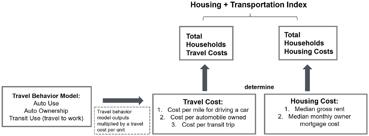
Figure 1 shows the variables needed to estimate housing and transportation costs. We include auto ownership costs (cost of auto ownership per household), driving costs (cost per mile driving per household), and public transportation costs (cost per transit trip) as the three primary sources of transportation costs, and consider rent costs and mortgage costs as the primary housing costs.

Figure 1.

Housing and transportation cost model.

The UT-Index uses a combination of demographic and travel-related data, mostly taken from national and local government sources that are publicly available. These include

American Community Survey 2015 to 2019 5-Year Estimates that provide summaries of demographic characteristics, housing characteristics, commuting characteristics, income, employment, and other variables.

U.S. Census TIGER/Line Shapefiles that provide geographic boundaries, characteristics, and the location of other features including roads and rivers.

Consumer Expenditure Surveys–Public Use Microdata (CES-PUMD) that summarize different types of automobile expenditures disaggregated by household income category.

General Transit Feed Specification (GTFS) data that contain transit route and schedule information for all fixed-route service in the Capital Metropolitan Transportation Authority (CapMetro) service area. CapMetro is the public transportation provider in Austin, TX.

Capital Area Rural Transportation System (CARTS) transit stops: CARTS provides transit service in some nonurbanized areas of the region. Their website lists bus stop addresses.

National Transit Database 2019 (NTD): NTD data summarize the financial, asset, and operating conditions of transit systems across the United States.

2015 CAMPO trip data: These origin–destination data originate from CAMPO’s travel demand model and summarize trip counts at the traffic analysis zone (TAZ) level.

Table 1 below summarizes the specific variables extracted from each data source. Mortgage and rent costs are obtained directly at the block-group level, whereas other variables must be converted to the block-group level from other spatial units using areal interpolation.

Table 1.

UT-Index Variables and Data Sources

Variable description	Source	Geographic level
Housing variables
Monthly costs for owners with a mortgage	2019 ACS	Block group
Median gross monthly rent for renters	2019 ACS	Block group
Transportation variables
Transit use	Number of transit commuters: 2019 ACS	Block group
	Fare revenue: 2019 NTD	Data at county level converted to block-group level
	Service location: CapMetro GTFS, CARTS transit stops	Geographic location (latitude, longitude)
Auto ownership	2019 CES-PUMD	State level by income group
Auto use	2015 CAMPO all-purpose trips between production and attraction zones	Traffic analysis zone level converted to block group

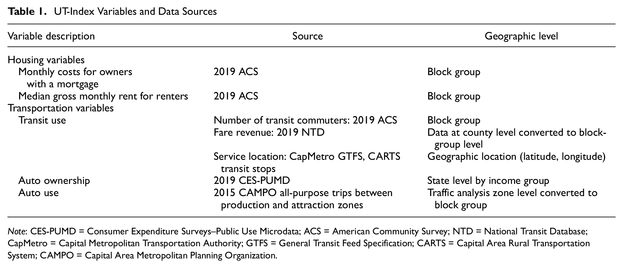
Note: CES-PUMD = Consumer Expenditure Surveys–Public Use Microdata; ACS = American Community Survey; NTD = National Transit Database; CapMetro = Capital Metropolitan Transportation Authority; GTFS = General Transit Feed Specification; CARTS = Capital Area Rural Transportation System; CAMPO = Capital Area Metropolitan Planning Organization.

Although the data used here are localized, the entire process and logic of the UT-Index could be employed elsewhere in the United States, where similar travel demand and automobile cost information are available. The only somewhat difficult-to-obtain dataset used in the UT-Index was automobile travel demand, sourced from a regional travel demand model. All other data, including transit revenue, transit service locations, transit commuters, and auto ownership costs, were derived from publicly available datasets. Our strategy for making this index more contextually appropriate was to narrow the geographic scope of all the data to Texas or smaller. For example, we only looked at the total public transit revenue shared by all three local public transit providers in the target region. We also used consumer expenditure results for Texas from the CES dataset.

Housing Costs

We took housing costs from the ACS 2015 to 2019 5-year estimates. We averaged monthly owner costs for owner-occupied units and monthly gross rent for renter-occupied units weighted by the ratio of the owner- to renter-occupied housing units from the tenure variable for each block group. Total costs were divided by the number of housing units to derive an average housing cost per household at the block-group level.

Public Transit Costs

We allocated total fare revenue gleaned from the NTD to each county, weighted by their proportion of transit stops, to obtain total public transit costs. Household transit costs at the block-group level were estimated by converting transportation revenues from the county to the block-group level using the ratio of block-group public transportation commuters to county public transportation commuters taken from the ACS.

Auto Ownership and Use Costs

We produced automobile ownership and use costs separately for each of the five household income categories ($ 0–20,000, $20,000–40,000, $40,000–60,000, $60,000–100,000, and $100,000 and above). We classified expenditures related to the purchase and operation of cars and trucks into the following five categories:

Outlay purchase: average outlays for vehicle purchases including down payment, principal, or if not financed, the purchase amount;

Finance: average annual payment of other finance expenses related to the vehicle;

Insurance: average annual insurance paid;

Fuel: average annual costs of fuel used in passenger vehicles; and

Drivability (maintenance + service): average annual cost of keeping the vehicle in a drivable condition, including maintenance, repairs, vehicle rental, leases, licenses, and other service charges.

We calculated total automobile ownership and use costs at the block-group level using Equation 1,

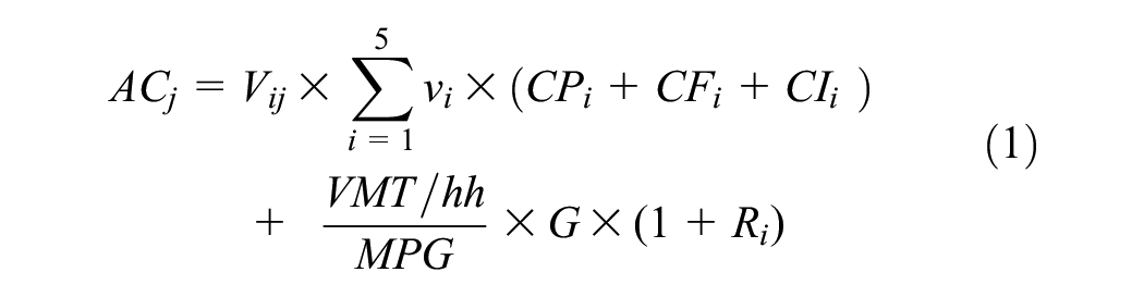
\begin{matrix} A C_{j} = V_{ij} \times \sum_{i = 1}^{5} v_{i} \times ({CP}_{i} + {CF}_{i} + {CI}_{i}) \\ + \frac{VMT / hh}{MPG} \times G \times (1 + R_{i}) \end{matrix}

(1)

where j indexes block groups, i indexes the five income categories, Vij is the total number of vehicles owned by income category i in block group j, v_i represents the average number of vehicles owned per household for income category i, CP_i represents per vehicle outlay purchase cost (excluding finance) for income category i, CF_i represents per vehicle finance charges for income category i, CI_i represents per vehicle annual insurance costs for income category i, VMT/hh is vehicle miles traveled per household at the block-group level, MPG is the average fuel economy in Texas in 2017 = 22.1 mpg, G is the average cost of gasoline per gallon in the Gulf Coast for 2019 = $2.691, and R_i is the average ratio of drivability to fuel costs.

Input data came from multiple sources. We used the CES-PUMD state weights for Texas to extract vehicle outlay purchase cost, finance charges, insurance costs, and the ratio of maintenance and service costs to fuel costs. We used VMT data gleaned from base year 2015 trip and skim tables at the TAZ level obtained from CAMPO, downsampling to the block-group level using areal interpolation. Average fuel economy data came from the 2017 National Household Travel Survey (NHTS) dataset. Average fuel price was taken from the Energy Information Administration.

To calculate total transportation costs for each block group, we used ACS estimates of automobile ownership by income at the tract level. Block-group data were not available with acceptable margins of error. Ultimately, mean household automobile ownership and use costs in each tract were generated by dividing the average weighted total expenditures at the tract level by the number of households at the tract level. We then assigned the average expenditures in each tract to the corresponding block groups within that tract to produce household automobile ownership expenditures at the block-group level.

Identifying Choice and Constraint Using Mode Switch Propensity

We gleaned the mode switch propensity score from several NHTS questions. Specifically, the NHTS includes questions asking about mode choice and financial burdens that we used to identify block groups where residents are able to switch to public transit, walking, and cycling. The three NHTS questions separately ask whether a household uses public transit, walks, or bikes to reduce the “financial burden of travel.” Responses are on a Likert scale ranging from “strongly agree” to “strongly disagree.” These questions mix elements of choice and constraint. Some households may switch modes to reduce the financial burden of travel but may not strictly need to save money—they may simply value thrift. The households would score high on mode switch propensity but are not actually constrained in their choices. Others may want to switch modes but simply cannot, because of infrastructure deficiencies, levels of service, feelings of safety, or other factors. These households would score low but in fact are substantially constrained. Investigating overall mode switch propensity scores alongside other demographic indicators should shed light on whether households are more likely to experience freedom of choice or to be constrained.

We used a binary logit model to identify NHTS variables associated with mode switch propensity. Our dependent variable was binary. If a respondent selected that they “agreed” or “strongly agreed” that they mode switch in any of the three cases to reduce financial burdens, we identified them as high-propensity households. We selected independent variables known to affect travel behavior, including income and race, car ownership, trip purpose, travel time, population density, and transit use. We focused exclusively on work-related trips to ensure consistency with the variables employed in the UT-Index. The binary logit model is summarized in Equation 2,

P (y_{j}) = (1 + e^{- [b_{0} + \sum_{i = 1}^{8} (b_{i} \times X_{ij})]})^{- 1}

(2)

where

j indexes block groups;

y_j represents the binary dependent variable for mode switch, as described above;

b₀ is constant obtained during model estimation;

b_i represents the coefficient for the ith independent variable; and

x_ij represents value of the ith independent variable in block group j.

The independent variables include automobile sufficiency, household income, daily travel distance, population density, travel time, transit users, householders by race, and householders by ethnicity.

We used the final model to estimate mode switch propensity for each block group using ACS variables corresponding to those employed during estimation. These weighted variables were analogous to the independent variables used in the logit model. The coefficient assigned to each variable corresponded to the respective coefficient values derived from the logit model. Variables related to aggregated travel times and the size of households in relation to available vehicles were converted from the census tract level to the block-group level.

Results and Discussion

H+T Cost Modeling Comparison

Overall, the UT-Index-estimated total H+T cost had a similar distribution to CNT’s final estimated H+T costs (Figure 2). Both the CNT and UT-Index showed that the H+T costs per household were higher in the western part of the region compared with the east. The results corresponded to the skewed spatial distribution of housing costs and income resulting from myriad policies that have shaped the spatial distribution of opportunity in the region. For example, the notorious “1928 Austin City Plan,” effected de facto racial zoning by placing all services and facilities available to Black people in East Austin while refusing to provide services for Black residents living elsewhere in the city ( 29 – 31 ). East Austin and parts of south Austin were subsequently “redlined,” making obtaining real-estate financing and attendant wealth-building difficult or impossible for Austin’s Black residents. Generational racialized health disparities have persisted in Austin and elsewhere throughout the 20th and 21st centuries ( 31 ).

Figure 2.

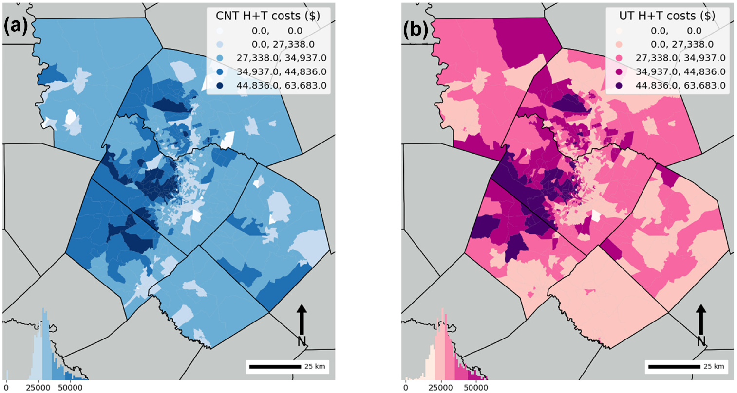
Choropleth maps showing Five total H+T cost categories defined using Jenks natural breaks for (a) the Center for Neighborhood Technology’s (CNT) Housing and Transportation (H+T) cost index and (b) our UT-Index estimates.

The differences between the two indices are likely the result of using different data sources. The UT-Index used more complete public transit information and locally tailored estimates of automobile travel and automobile ownership costs. Higher-income households residing in the western region incurred higher housing costs, owned more automobiles, and traveled further than households located in the east. But these results tell us little about which households are burdened.

In relation to the spatial pattern of transportation costs, households with any public transit costs at all were concentrated in central Austin. This result is not surprising, since this is where service is concentrated as well, as shown in Figure 3. The locations with the highest costs were generally populated by students.

Figure 3.

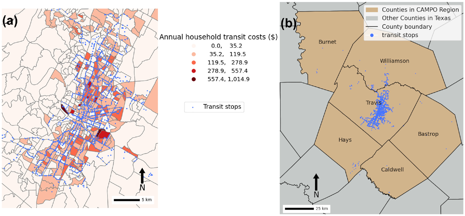
(a) Annual public transit costs per household in Austin and (b) the distribution of transit stops in the study region.

Key Factors Contributing to Mode Switch Propensity

The mode switch propensity model results are shown in Table 2. They show that automobile sufficiency, household income, and travel distance (measured as VMT) were all associated with a lower likelihood of mode switching. These results were all in the expected direction. If a household had greater automobile and financial resources, they were less likely to mode switch. Additionally, the results demonstrated that all households with householders of color were more likely than white households to mode switch, even when controlling for income. Historical distributions of opportunity and ongoing racism and discrimination are likely to account for these differences. Our land-use variable—population density—showed the expected relationship as well. In denser locations, NHTS respondents were more likely to switch modes, all else equal.

Table 2.

NHTS Logit Model Showing the Key Factors Contributing to Mode Switch Propensity

	Coefficient	p-value	Standard error
Intercept	0.519	0.000	0.024
Dummy: Number of household vehicles < Household size	Reference group
Dummy: Number of household vehicles ≥ Household size	−0.502	0.000	0.009
Dummy: Household Income Group 1: (<$75,000)	Reference group
Dummy: Household Income Group 2 (≥$75,000)	−0.472	0.000	0.005
Daily VMT	−0.006	0.000	0.000
Population density (persons/mi²)	0.00005	0.000	0.000
Travel time (min)	0.001	0.000	0.000
Dummy: Transit user	Reference group
Dummy: Nontransit use	−1.825	0.000	0.002
Dummy: White householder	Reference group
Dummy: Black householder	0.290	0.000	0.011
Dummy: Asian householder	0.605	0.000	0.012
Dummy: Multiple race householder	0.365	0.000	0.016
Dummy: Other race householder	0.550	0.000	0.013
Dummy: Non-Hispanic Householder	Reference group
Dummy: Hispanic householder	0.309	0.000	0.007
N = 921,121 McFadden’s rho²: 0.04 Adjusted rho²: 0.06

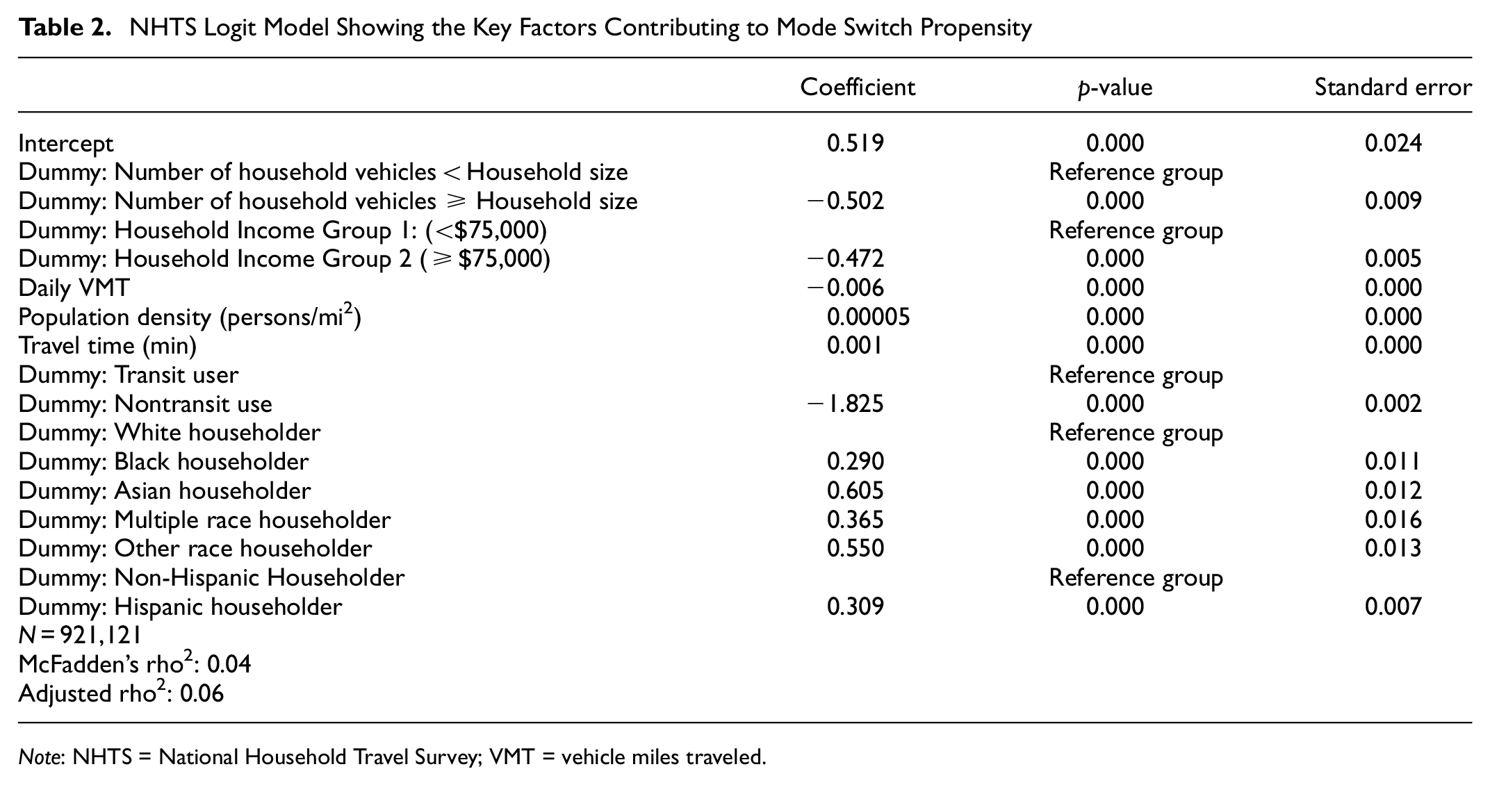
Note: NHTS = National Household Travel Survey; VMT = vehicle miles traveled.

Using the coefficients from Table 2, we calculated a mode switch propensity at the block-group level for the entire region. In line with affordability benchmarks ( 32 ), where H+T costs should not exceed 45% of a household’s income, we classified areas where H+T costs surpassed this threshold as those with high H+T costs. High mode-switch propensity households were those with a mode switch probability equal to or greater than 50%.

Figure 4 shows four distinct household types based on their H+T costs and mode switch propensity:

High mode switch propensity-High cost burden (HH): mode switch propensity > 50% and combined H+T share > 45%

High mode switch propensity-Low cost burden (HL): mode switch propensity > 50% and combined H+T share < 45%

Low mode switch propensity-High cost burden (LH): mode switch propensity < 50% and combined H+T share > 45%

Low mode switch propensity-Low cost burden (LL): mode switch propensity < 50% and combined H+T share < 45%

Figure 4.

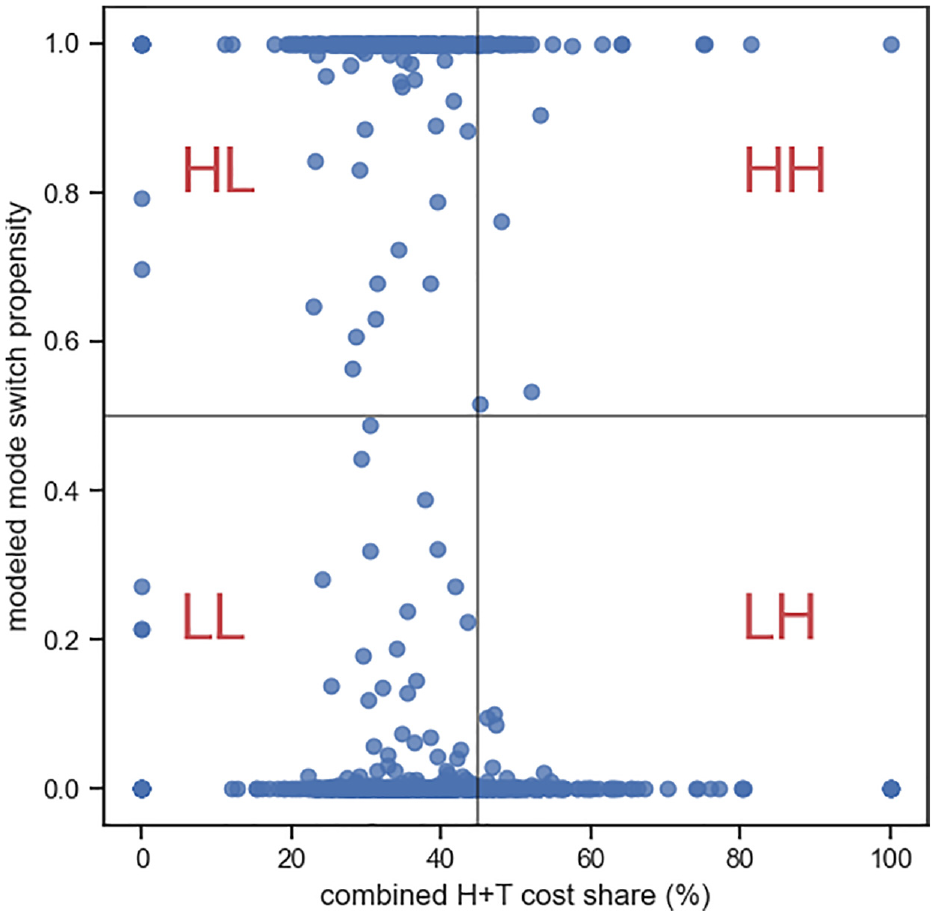
Modeled travel burden probability and combined H+T costs for all block groups.

Choice and Constrained Travelers in the CAMPO Region

Table 3 summarizes household demographics for block groups in each of the four categories. The table demonstrates the importance of income for determining the true degree of choice versus constraint faced by a household. Block groups characterized by high H+T cost burdens (the first two rows of Table 3) had similarly low average incomes and similar automobile ownership, but quite different travel patterns, depending on their mode switch propensity. HH households consumed about 50% of the VMT that LH households did. The relatively low amount of driving that HH households undertook probably reflects some combination of the viability of available alternatives or some degree of suppressed travel demand. LH households, on the other hand, generally did not mode switch to reduce the financial burden of travel. But rather than indicating relative ease, the low propensity to switch might reflect lower available alternatives to driving. Locked into automobile ownership and with few alternatives available, LH households are effectively forced to drive to access opportunities. Notably, households with a similar mode switch propensity experienced similar work-related VMT, regardless of the cost burdens. This result reduces the likelihood that either HH or LH households experience suppressed travel demand, on average.

Table 3.

Income and Vehicle Travel Distances by Mode Switch Propensity at the Household Level

	Average annual income ($)	Annual work-related VMT	Automobile ownership	Number of block groups
HH	43,098	9,263	1.4	43
LH	46,136	17,511	1.5	132
HL	82,989	8,533	1.6	294
LL	92,824	15,800	1.7	525

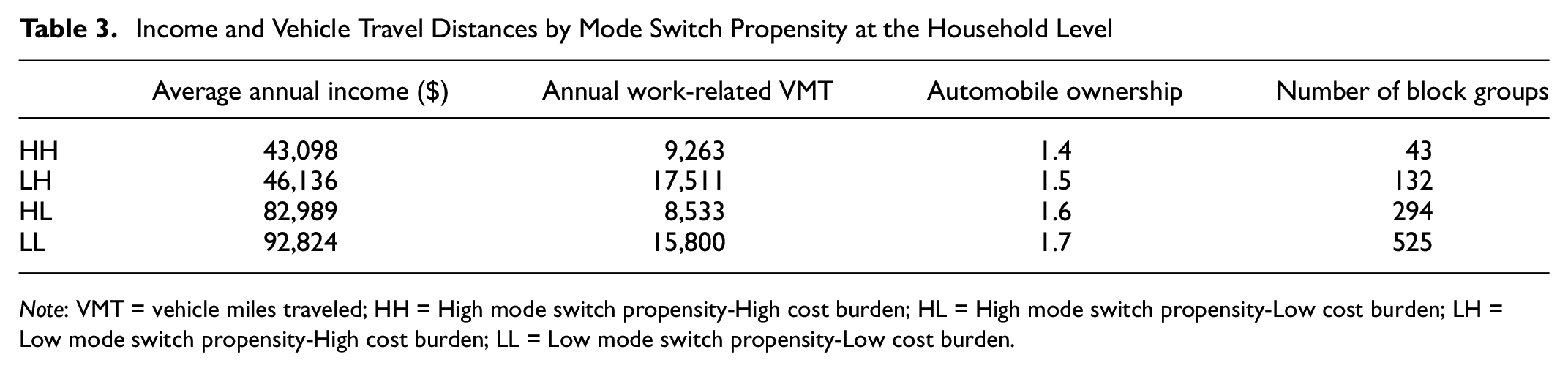
Note: VMT = vehicle miles traveled; HH = High mode switch propensity-High cost burden; HL = High mode switch propensity-Low cost burden; LH = Low mode switch propensity-High cost burden; LL = Low mode switch propensity-Low cost burden.

The main difference between block groups characterized by low and high H+T cost burdens was income. On average, higher incomes did not translate to higher H+T cost shares. Block groups characterized by low H+T cost burdens (the last two rows of Table 3) had relatively high average incomes—approximately double those with low cost burdens. The annual VMT of these block groups was also bifurcated. HL households had about 50% of the annual work-related VMT as LL households. HL households had a higher propensity to mode switch and were thus likely have more viable alternatives as opposed to a genuine need to save money or suppress travel demand.

The results demonstrated that income was only one dimension of choice and constraint. There appeared to be at least some low-income households with high H+T cost shares that were able to mode switch to reduce financial burdens. However, other high H+T cost households faced limited travel alternatives, most likely leading to involuntary expenditures and forced car ownership ( 33 ). Accordingly, households characterized by high H+T costs cannot be automatically classified as constrained. Rather, it is necessary to incorporate information about other travel-related burdens and constraints to make this determination.

There is, of course, a spatial dimension to these patterns. Figure 5 shows the spatial distribution of block groups in each of the four categories with the U.S. Census Bureau’s urbanized area definition overlaid ( 34 ). Not surprisingly, those block groups identified as experiencing high mode switch propensity were concentrated largely within the region’s urbanized area. By and large, these represent relatively dense locations where automobile alternatives are likely to be more viable. Even relatively small Bastrop, TX (population approximately 10,000, the easternmost urbanized location) contains a walkable downtown street grid. Outside of the urbanized area, where land use is likely to be more rural in character, there was a mix of households with low mode switch propensity but both high and low H+T costs. Accordingly, people either earned enough that their H+T costs were low as a share of income, or they were unable to mode switch and faced relatively high H+T costs. Numerically, a majority of block groups were categorized as LL, suggesting that arguments about reducing transportation costs are likely to have little resonance among that population.

Figure 5.

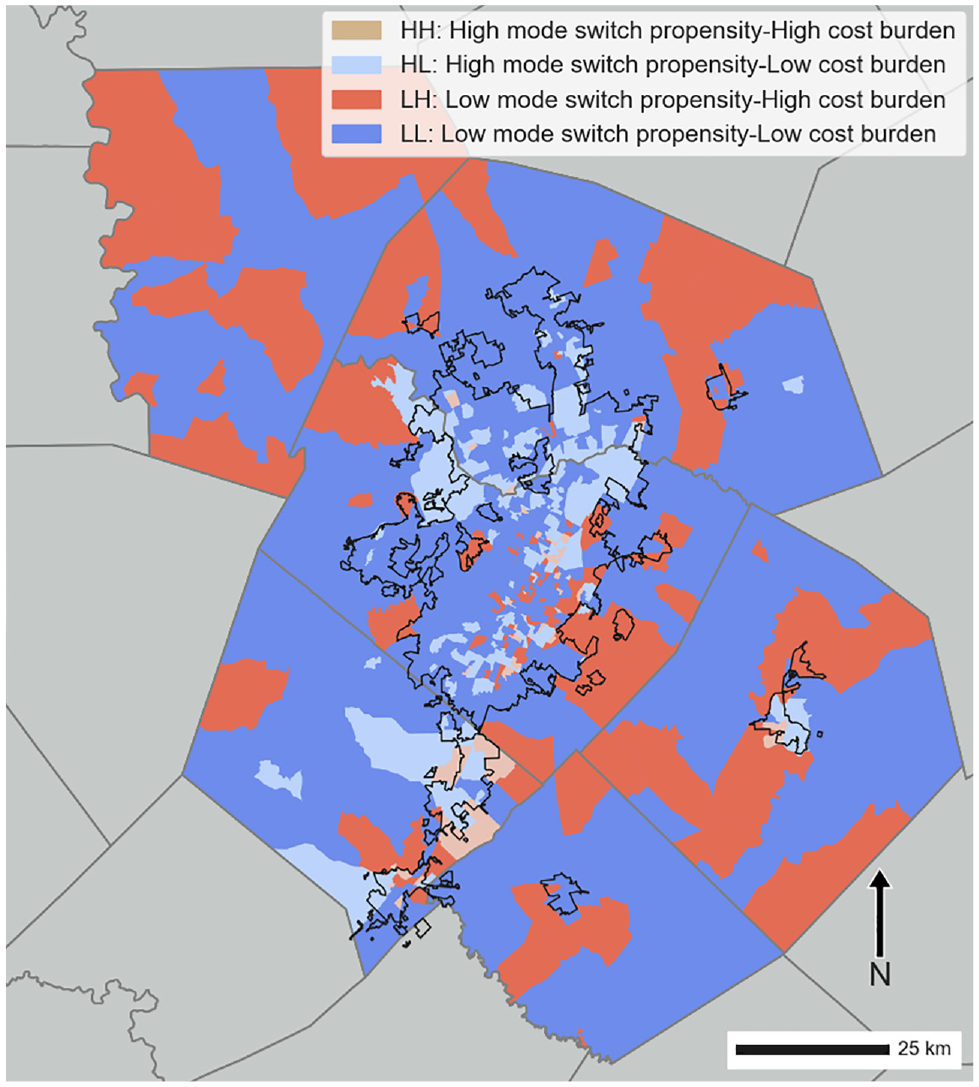
Spatial distribution of mode switch propensity and H+T costs. The black outline represents the U.S. Census Bureau’s urbanized area definition.

Drilling down further into demographic composition, racial and ethnic patterns were also evident in the different categories of mode switch propensity and H+T cost burdens, as summarized in Figure 6. In general, a high proportion of white and Asian households were located in block groups that had low H+T cost shares compared with other racial and ethnic groups. Specifically, the share of white residents in block groups experiencing low H+T costs was 87% of the total white population. The same value for Asian households was 88.5%. On the other hand, only 78.5% of Hispanic or Latino residents and 75.9% of Black residents were located in low H+T block groups. These results highlight a disparity in the distribution of households experiencing constraints, with white and Asian households experiencing a notably lower burden compared with other racialized populations. In part these results reflect known disparities in income and wealth that have historical and ongoing causes ( 35 ), and ongoing issues with spatial mismatch and residential displacement ( 36 , 37 ). The results presented here might actually underestimate true H+T cost burdens, since they do not account for the differential treatment faced in the automobile lending market by borrowers of color, including higher interest rates and inflated purchase costs ( 38 ). We relied on statewide averages across all automobile owners, which were the only data available.

Figure 6.

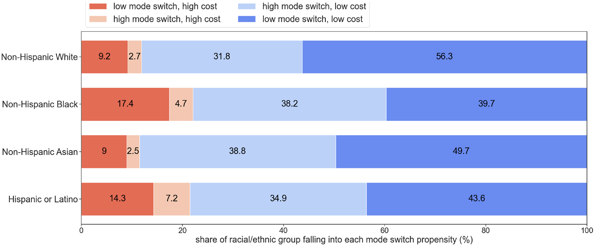
Share of racial/ethnic group falling into each mode switch propensity category.

Conclusions

This study has made two main contributions to the literature on H+T costs: 1) building and applying a local, context-dependent, and reproducible H+T cost model and 2) identifying choice/constrained households using H+T costs and mode switch propensity. The former fills the gap in estimating H+T costs using local datasets, whereas the latter problematizes the use of H+T cost alone to assess transportation disadvantage. Specifically, we developed the UT-Index using data gleaned largely from publicly available sources and drawing inspiration from the two leading H+T cost modeling efforts undertaken by CNT and HUD. The UT-Index reflected more nuanced H+T cost differences that corresponded to local conditions.

When considering how to translate these or similar results into practice, local agencies may face limited staff capacity or expertise. One possible solution is to partner with institutions of higher education to leverage their professional resources. Fields et al. ( 39 ) report that providing educational institutions with an opportunity for capstone or research programs can both help the next generation of professionals gain an early understanding of the skills needed by agencies and compensate for staffing shortages. In other words, agencies need not possess financial resources to take advantage of collaborations with colleges and universities.

Unlike the two existing tools authored by CNT and HUD, we did not rely on fictional household compositions to identify vulnerable groups. Instead, we spatially distinguished between choice and constrained households using a combination of the UT-Index results and NHTS data. Households experiencing a higher degree of choice resided close to populated cities. These households included those with both high and low H+T cost burdens and they generated similar amounts of work-related VMT, suggesting that households with a high ability to switch modes do not experience much suppressed travel, even though they have high H+T costs. Our work will allow decision makers and advocates to identify specific locations in a region where certain H+T cost conditions and travel behaviors dominate. These locations can subsequently be targeted for mitigation. By summarizing results for typical household profiles, existing H+T cost tools simply do not offer the same information that the UT-Index does.

Our results were limited in various ways by the available data. For example, we obtained mode switch propensity scores by using questions from the NHTS, specifically focusing on the financial aspects of travel burdens. However, individuals with low mode switch propensity may encounter more than just financial challenges. Our study demonstrated how this group often lacks access to multiple transportation options for reaching their destinations. In addition, most literature has highlighted a wide variety of travel barriers that people may encounter in addition to the cost of travel, such as mobility problems for people with disabilities and safety concerns when using public transit ( 40 – 44 ).

Travel and activity surveys rarely include specific questions about different types of travel burdens and their underlying causes. The more precise survey questions are in relation to travel burdens, the more accurate mode switch propensity scores can become. As suggested by Luiu et al. ( 45 ), it is crucial to pay attention to individuals’“inability” to complete necessary travel, where this inability can be attributed to health conditions, physical disabilities, or the absence of suitable travel services or tools. Indeed, empirical work has underscored that various social characteristics such as race/ethnicity, gender identity, sexual orientation, language proficiency, immigration status, and disability status can produce travel barriers ( 43 , 44 , 46 –50). Therefore, we suggest that transportation agencies include travel burden questions in relevant surveys, including but not limited to affordability, safety, travel comfort, language proficiency, disability status, gender identity, and other relevant factors.

The absence of these questions means that we cannot link real-world travel burdens to the mode switch propensity we estimated. Although the intersection of H+T costs and mode switch propensity appeared to produce reasonable results in relation to the spatial location of travelers in each of the four categories, directly measuring the extent to which high and low mode switch propensity were associated with travel burdens is still unattainable. In other words, did respondents with a high mode switch propensity experience limited travel or suppressed demand? Or were alternatives sufficient to meet their daily needs? Conversely, did respondents with a low propensity feel constrained to use the automobile to meet most or all of their travel needs, or did they freely choose those travel behaviors? Emerging approaches that more directly address travel problems present a promising approach for differentiating between these possibilities, but questions would need to be incorporated into large-scale regional or national surveys to be of use (e.g., Singer and Martens [ 51 ]).

Finally, our work suffers from issues related to missing data and aggregation bias. CapMetro implemented a new shared-ride shuttle service called “Pick Up” within various zones of its service area beginning in 2017. Our estimates of public transit service coverage did not include this service because no data are available on its relative use across space. Issues of aggregation bias arose because of the different spatial units inherent in the various datasets we used. To apply results gleaned from the NHTS to our case, we had to conduct the analysis at the block-group level. This translation involved using aggregate ACS shares to estimate probabilities gleaned from a model that was itself estimated from individual-level NHTS data. As a result, we were only able to classify block groups into our four categories. Ideally, we would be able to generate some information about the distribution of people across the four groups. In some sense, this tradeoff is impossible to address using currently available data source. The public use microdata sample is available, but geographic information about respondents is limited to the public use microdata area (PUMA) level. A single county sometimes contains several PUMAs, but the PUMA definition is so coarse as to prevent linking local land-use or transportation characteristics to it. Again, original data collection is likely to offer a way forward.

Footnotes

Author Contributions

The authors confirm contribution to the paper as follows: study conception and design: M. Situ, A. Karner; data collection: M. Situ; analysis and interpretation of results: M. Situ, A. Karner; draft manuscript preparation: M. Situ, A. Karner. All authors reviewed the results and approved the final version of the manuscript.

Declaration of Conflicting Interests

The authors declared no potential conflicts of interest with respect to the research, authorship, and/or publication of this article.

Funding

The authors disclosed receipt of the following financial support for the research, authorship, and/or publication of this article: Support for this work was provided by the City of Austin Transportation Department under master agreement number UTA19-000382.

ORCID iDs

Minyu Situ

Alex Karner

References

Wetzstein

The Global Urban Housing Affordability Crisis. Urban Studies, Vol. 54, No. 14, 2017, pp. 3159–3177. https://doi.org/10.1177/0042098017711649.

Rohe

W. M.

Tackling the Housing Affordability Crisis. Housing Policy Debate, Vol. 27, No. 3, 2017, pp. 490–494. https://doi.org/10.1080/10511482.2017.1298214.

Tretter

Mueller

E. J.

Heyman

Yimbyism, the Environment, and the Remaking of Race and Class Coalitions in Austin, TX. International Journal of Urban and Regional Research, Vol. 46, No. 2, 2022, pp. 312–318. https://doi.org/10.1111/1468-2427.13066.

Hamidi

Ewing

Is Sprawl Affordable for Americans?: Exploring the Association Between Housing and Transportation Affordability and Urban Sprawl. Transportation Research Record: Journal of the Transportation Research Board, 2015. 2500: 75–79.

Haas

P. M.

Newmark

G. L.

Morrison

T. R.

Untangling Housing Cost and Transportation Interactions: The Location Affordability Index Model—Version 2 (LAIM2). Housing Policy Debate, Vol. 26, No. 4–5, 2016, pp. 568–582. https://doi.org/10.1080/10511482.2016.1158199.

Haas

P. M.

Makarewicz

Benedict

Bernstein

Estimating Transportation Costs by Characteristics of Neighborhood and Household. Transportation Research Record: Journal of the Transportation Research Board, 2008. 2077: 62–70.

Holtzclaw

Clear

Dittmar

Goldstein

Haas

Location Efficiency: Neighborhood and Socio-Economic Characteristics Determine Auto Ownership and Use - Studies in Chicago, Los Angeles and San Francisco. Transportation Planning and Technology, Vol. 25, No. 1, 2002, pp. 1–27. https://doi.org/10.1080/03081060290032033.

Koschinsky

Talen

Location Efficiency and Affordability: A National Analysis of Walkable Access and HUD-Assisted Housing. Housing Policy Debate, Vol. 26, No. 4–5, 2016, pp. 835–863. https://doi.org/10.1080/10511482.2015.1137965.

Center for Neighborhood Technology. H+T Index Methods. Center for Neighborhood Technology. Chicago, IL, 2017.

10.

Garrett

Taylor

Reconsidering Social Equity in Public Transit. Berkeley Planning Journal, Vol. 13, No. 1, 1999, pp. 6–27. https://doi.org/10.5070/BP313113028.

11.

Brown

A. E.

Car-Less or Car-Free? Socioeconomic and Mobility Differences among Zero-Car Households. Transport Policy, Vol. 60, 2017, pp. 152–159. https://doi.org/10.1016/j.tranpol.2017.09.016.

12.

Johnson

Currie

Stanley

Measures of Disadvantage: Is Car Ownership a Good Indicator?

Social Indicators Research, Vol. 97, No. 3, 2010, pp. 439–450. https://doi.org/10.1007/s11205-009-9510-1.

13.

Mattioli

Where Sustainable Transport and Social Exclusion Meet: Households Without Cars and Car Dependence in Great Britain. Journal of Environmental Policy & Planning, Vol. 16, No. 3, 2014, pp. 379–400. https://doi.org/10.1080/1523908X.2013.858592.

14.

Ewing

Cervero

Travel and the Built Environment. Journal of the American Planning Association, Vol. 76, No. 3, 2010, pp. 265–294. https://doi.org/10.1080/01944361003766766.

15.

Saberi

Amoh-Gyimah

Smith

Arunachalam

Measuring Housing and Transportation Affordability: A Case Study of Melbourne, Australia. Journal of Transport Geography, Vol. 65, 2017, pp. 134–146. https://doi.org/10.1016/j.jtrangeo.2017.10.007.

16.

Dewita

Yen

B. T. H.

Burke

The Effect of Transport Cost on Housing Affordability: Experiences from the Bandung Metropolitan Area, Indonesia. Land Use Policy, Vol. 79, 2018, pp. 507–519. https://doi.org/10.1016/j.landusepol.2018.08.043.

17.

Hartell

A. M.

Evaluating the Concept of Location Affordability: Recent Data on the Relationship Between Transportation, Housing, and Urban Form. Housing Policy Debate, Vol. 27, No. 3, 2017, pp. 356–371. https://doi.org/10.1080/10511482.2016.1220402.

18.

CNT, and Surface Transportation Policy Project. Driven to Spend: The Impact of Sprawl on Household Transportation Expenses. Surface Transportation Policy Project, Washington, D.C. Center for Neighborhood Technology, Chicago, IL, 2000.

19.

Haas

P. M.

Morse

Becker

Young

Esling

The Influence of Spatial and Household Characteristics on Household Transportation Costs. Research in Transportation Business & Management, Vol. 7, 2013, pp. 14–26. https://doi.org/10.1016/j.rtbm.2013.03.004.

20.

HUD. Location Affordability Index - Documentation. https://www.hudexchange.info/programs/location-affordability-index/documentation. Accessed November 3, 2021.

21.

Guerra

Kirschen

Housing Plus Transportation Affordability Indices: Uses, Opportunities, and Challenges. Discussion Paper, Publication 2016–14. International Transport Forum, Paris, France, 2016.

22.

Ganning

J. P.

It’s Good but Is It Right? An Under-the-Hood View of the Location Affordability Index. Housing Policy Debate, Vol. 27, No. 6, 2017, pp. 807–824. https://doi.org/10.1080/10511482.2017.1312478.

23.

Tiznado-Aitken

Lucas

Muñoz

J. C.

Hurtubia

Freedom of Choice? Social and Spatial Disparities on Combined Housing and Transport Affordability. Transport Policy, Vol. 122, 2022, pp. 39–53. https://doi.org/10.1016/j.tranpol.2022.04.005.

24.

Jirón

Carrasco

J.-A.

Rebolledo

Observing Gendered Interdependent Mobility Barriers Using an Ethnographic and Time Use Approach. Transportation Research Part A: Policy and Practice, Vol. 140, 2020, pp. 204–214. https://doi.org/10.1016/j.tra.2020.08.018.

25.

Kawabata

Shen

Commuting Inequality between Cars and Public Transit: The Case of the San Francisco Bay Area, 1990-2000. Urban Studies, Vol. 44, No. 9, 2007, pp. 1759–1780.

26.

Banister

Equity and Acceptability in Internalising the Social Costs of Transport. EMCT, Internalising the Social Costs of Transport, 1994, pp. 153–175.

27.

Currie

Senbergs

Exploring Forced Car Ownership in Metropolitan Melbourne. 2007.

28.

Handy

Weston

Mokhtarian

P. L.

Driving by Choice or Necessity?

Transportation Research Part A: Policy and Practice, Vol. 39, No. 2, 2005, pp. 183–203. https://doi.org/10.1016/j.tra.2004.09.002.

29.

Busch

A. M.

The Perils of Participatory Planning: Space, Race, Environmentalism, and History in “Austin Tomorrow.”

Journal of Planning History, Vol. 15, No. 2, 2016, pp. 87–107. https://doi.org/10.1177/1538513215590500.

30.

Busch

Building “A City of Upper-Middle-Class Citizens”: Labor Markets, Segregation, and Growth in Austin, Texas, 1950–1973. Journal of Urban History, Vol. 39, No. 5, 2013, pp. 975–996. https://doi.org/10.1177/0096144213479324.

31.

Hidalgo

Keep Austin…White? How Equitable Development Can Save Austin, Texas from Its Racist Past and Homogenized Future. Texas A&M Journal of Property Law, Vol. 9, No. 1, 2023, pp. 109–145. https://doi.org/10.37419/JPL.V9.I1.5.

32.

CNT. CNT H+T Index. https://cnt.org/tools/housing-and-transportation-affordability-index. Accessed November 13, 2021.

33.

Delbosc

Currie

Choice and Disadvantage in Low-Car Ownership Households. Transport Policy, Vol. 23, 2012, pp. 8–14. https://doi.org/10.1016/j.tranpol.2012.06.006.

34.

U.S. Census Bureau. Urban and Rural. https://www.census.gov/programs-surveys/geography/guidance/geo-areas/urban-rural.html#:~:text=To%20qualify%20as%20an%20urban,population%20of%20at%20least%205%2C000.

35.

Hamilton

Darity

Can ‘Baby Bonds’ Eliminate the Racial Wealth Gap in Putative Post-Racial America?

The Review of Black Political Economy, Vol. 37, No. 3–4, 2010, pp. 207–216. https://doi.org/10.1007/s12114-010-9063-1.

36.

Allen

Farber

Suburbanization of Transport Poverty. Annals of the American Association of Geographers, Vol. 111, No. 6, 2021, pp. 1833–1850. https://doi.org/10.1080/24694452.2020.1859981.

37.

Gobillon

Selod

Spatial Mismatch, Poverty, and Vulnerable Populations. In Handbook of Regional Science ( M. M.

Fischer

Nijkamp

, eds.), Springer, Berlin, Heidelberg, 2021, pp. 573–588.

38.

Livingston

Ross

Cars and Jails: Freedom Dreams, Debt and Carcerality. OR Books, New York, NY; London, 2022.

39.

Fields

N. L.

Miller

V. J.

Cronley

Hyun

Mattingly

S. P.

Khademi

Nargesi

S. R. R.

Williams

Interprofessional Collaboration to Promote Transportation Equity for Environmental Justice Populations: A Mixed Methods Study of Civil Engineers, Transportation Planners, and Social Workers’ Perspectives. Transportation Research Interdisciplinary Perspectives, Vol. 5, 2020, p. 100110. https://doi.org/10.1016/j.trip.2020.100110.

40.

Bezyak

J. L.

Sabella

S. A.

Gattis

R. H.

Public Transportation: An Investigation of Barriers for People with Disabilities. Journal of Disability Policy Studies, Vol. 28, No. 1, 2017, pp. 52–60. https://doi.org/10.1177/1044207317702070.

41.

Eisenberg

Heider

Gould

Jones

Are Communities in the United States Planning for Pedestrians with Disabilities? Findings from a Systematic Evaluation of Local Government Barrier Removal Plans. Cities, Vol. 102, 2020, p. 102720. https://doi.org/10.1016/j.cities.2020.102720.

42.

Lubitow

Rainer

Bassett

Exclusion and Vulnerability on Public Transit: Experiences of Transit Dependent Riders in Portland, Oregon. Mobilities, Vol. 12, No. 6, 2017, pp. 924–937. https://doi.org/10.1080/17450101.2016.1253816.

43.

Prescott

Labbé

Miller

W. C.

Borisoff

Feick

Mortenson

W. B.

Factors That Affect the Ability of People with Disabilities to Walk or Wheel to Destinations in Their Community: A Scoping Review. Transport Reviews, Vol. 40, No. 5, 2020, pp. 646–669. https://doi.org/10.1080/01441647.2020.1748139.

44.

Loukaitou-Sideris

Fear and Safety in Transit Environments from the Women’s Perspective. Security Journal, Vol. 27, 2014, pp. 242–256.

45.

Luiu

Tight

Burrow

The Unmet Travel Needs of the Older Population: A Review of the Literature. Transport Reviews, Vol. 37, No. 4, 2017, pp. 488–506.

46.

Liu

C. Y.

Painter

Travel Behavior among Latino Immigrants: The Role of Ethnic Concentration and Ethnic Employment. Journal of Planning Education and Research, Vol. 32, No. 1, 2012, pp. 62–80.

47.

Lubitow

Tompkins

Feldman

Sustainable Cycling for All? Race and Gender–Based Bicycling Inequalities in Portland, Oregon. City & Community, Vol. 18, No. 4, 2019, pp. 1181–1202. https://doi.org/10.1111/cico.12470.

48.

Lubitow

Abelson

M. J.

Carpenter

Transforming Mobility Justice: Gendered Harassment and Violence on Transit. Journal of Transport Geography, Vol. 82, 2020, p. 102601.

49.

McDonald

N. C.

Travel and the Social Environment: Evidence from Alameda County, California. Transportation Research Part D: Transport and Environment, Vol. 12, No. 1, 2007, pp. 53–63.

50.

Zeitler

Buys

Mobility and Out-of-Home Activities of Older People Living in Suburban Environments: ‘Because I’m a Driver, I Don’t Have a Problem’. Ageing & Society, Vol. 35, No. 4, 2015, pp. 785–808.

51.

Singer

M. E.

Martens

Measuring Travel Problems: Testing a Novel Survey Tool in a Natural Experiment. Transportation Research Part D: Transport and Environment, Vol. 121, 2023, p. 103834. https://doi.org/10.1016/j.trd.2023.103834.

Choice or Constraint? A Locally Tailored Assessment of Housing and Transportation Costs in Central Texas

Abstract

Keywords

Prior Work on Housing and Transportation Costs

Critiques and Weaknesses of Existing H+T Cost Modeling

Gap in Capturing Constrained Travelers

Data and Methods

Housing Costs

Public Transit Costs

Auto Ownership and Use Costs

Identifying Choice and Constraint Using Mode Switch Propensity

Results and Discussion

H+T Cost Modeling Comparison

Key Factors Contributing to Mode Switch Propensity

Choice and Constrained Travelers in the CAMPO Region

Conclusions

Footnotes

Author Contributions

Declaration of Conflicting Interests

Funding

ORCID iDs

References