
Abstract
Understanding the response of a transportation system to disruptive events is significant for evaluating the resilience of the system. However, data collection during such events is always challenging, and the data volume is insufficient for building a robust model. Transfer learning provides an effective solution to this problem. In this study, we propose a floating car data (FCD) driven transfer learning framework for predicting the resilience of target transportation systems to similar disruptive events to those that have ever occurred in the source systems. The core of the framework is an unsupervised pattern extractor that combines the k-Shape clustering and Bayes inference methods for extracting resilience patterns from the FCD collected in the source systems during the disruption period. The extracted patterns can then be used to assist in the prediction of the resilience of the target systems. We examine the effectiveness of the proposed framework by conducting a case study under the context of the COVID-19 pandemic, in which the source domain cities include Antwerp and Bangkok, and the target domain city is Barcelona. Results show that the extracted resilience patterns can improve the prediction performance of transfer learning neural networks with less pre-event information and limited data volume.
Keywords
Large events such as concerts, sports events, pandemics, and inclement weather can affect citizens’ travel behavior, causing disturbance to transportation systems. For example, under heavy rainstorms, the average vehicle speed will reduce because of slippery road surfaces and impaired visibility. During the COVID-19 pandemic, the intervention policies and people’s awareness of self-protection led to a reduction in traffic volume on the road network. By leveraging the knowledge of transportation system resilience, governments are able to establish more comprehensive recovery policies and containment measures, which help build a robust transportation system in the long run. Therefore, understanding the resilience of transportation systems under such events to bring systems back to their normal state in a timely manner becomes imperative ( 1 ).
Estimating and predicting the resilience of transportation systems has been a challenge for researchers for decades. Bruneau et al. ( 2 ) proposed a quantitative framework to evaluate the seismic resilience of communities, and the four associated four characteristics (robustness, redundancy, resourcefulness, and rapidity) are soon transferred into the field of transportation systems. The “4R” framework describes the resilience patterns, including the performance drop phase and performance recovery phase, as well as the new state a system reaches. However, evaluating the resilience of a transportation system using these characteristics relies on the complete information of the system functionality before, during, and after the event. In addition, the description of the coarse-grained resilience characteristics of a traffic road network could not provide sufficient support for the establishment of preparedness and recovery measures. To provide comprehensive information on resilience patterns, collecting appropriate data and developing an effective method to predict resilience patterns during the entire disruption period from pre-event data becomes imminent.
The challenges of predicting resilience patterns are three-fold. Firstly, the data used should reflect the fine-grained performance of a transportation system and be able to capture the features of the system’s reaction to large events. Secondly, because of the lack of during and post-event information in the target transportation system, predicting a time series with the entire system functionality trend requires a proven method to fully leverage the additional information. Thirdly, a transfer learning strategy for dealing with the data insufficiency problem is necessary. However, to our best knowledge, the research on resilience pattern prediction is still limited, and none of the previous studies have focused on all three of these issues at once.
To fill in the aforementioned gaps, we propose a transfer learning framework for predicting transportation demand resilience using floating car data (FCD), which utilizes the learned knowledge and experiences of source cities to facilitate the prediction for target cities. FCD is collected by Global Positioning System (GPS)-equipped vehicles, which play a vital role in traffic data mining ( 3 ). Compared to traditional methods of collecting traffic data, FCD are provided by various types of vehicles in a city-wide road network in real-time and are more flexible than fixed road sensors and traffic cameras ( 4 ), which overcomes some technical and terrain limitations of certain areas. In addition, FCD usually contains multi-dimensional information, such as positions, speed, time, and traffic volume, which strongly support the research on intelligent transportation systems (ITSs) ( 5 ).
The proposed framework consists of a resilience pattern extractor and artificial neural networks, which can alleviate the problem of low model performance caused by inconsistent traffic volume distribution among different systems/cities and enable effective transfer learning for the target domain. The contributions of this study are three-fold:
a transfer learning model is developed to address the transportation demand resilience prediction problem in the context of limited available data;
an unsupervised method combining k-Shape clustering and Bayes inference is designed to extract resilience patterns from the FCD;
we conduct case studies on three cities by using the FCD before and after the occurrence of the COVID-19 pandemic.
The rest of the paper is structured as follows. The Related Literature section reviews previous research focusing on transportation resilience estimation and prediction as well as transfer learning methods in traffic prediction tasks. The Methodology section presents the FCD-driven transfer learning framework for transportation demand resilience. The Case Study and Experimental Design sections introduce the study areas and experimental setups. Then, the Results section discusses the experiment results. Finally, the Conclusions section draws some conclusions and points out limitations and future directions.
Related Literature
In this section, we first review the studies related to transportation resilience estimation and prediction. Then, we introduce the transfer learning methods and the applications of transfer learning in transportation prediction tasks found in the existing literature.
For the past decades, a considerable amount of research has been conducted to estimate the resilience of transportation systems, and various indicators have been selected. For example, topological measures based on complex network theory, which can represent the structural properties (e.g., connectivity and accessibility) of the network ( 6 ), have gained popularity as resilience indicators in previous studies ( 7 ). On the other hand, traffic-based indicators, such as network average travel time ( 8 , 9 ), average speed ( 10 ), and demand served ( 11 ), have also been adopted to overcome the drawbacks of the topology-based ones.
To observe the trends in resilience patterns, some researchers leveraged the power of regression models to approximate the whole time series of the traffic representatives. For instance, Zhu et al. ( 12 ) scrutinized the number of taxi trips and subway ridership in New York City before and after the impact of hurricanes and applied a logistic function to model the recovery rate. Although the regression models are computationally efficient and can approximate resilience patterns, they fell short in capturing the temporal dependencies of these patterns. Mojtahedi et al. ( 13 ) developed a time-dependent recovery rate regression model based on Cox’s proportional hazards regression model, focusing on the post-event reconstruction duration. However, their model only considered the overall recovery time, that is, the rapidity of the system, thereby neglecting other resilience features (e.g., robustness, resourcefulness, and redundancy). Consequently, it failed to elucidate the specific event impacts at various stages.
On the other hand, predicting event-free scenarios has received increasing attention as it can reflect the impact of large events more intuitively. Therefore, causal impact analysis has become an important approach to the study of transportation system resilience, which is instrumental in evaluating the causal effect of a particular intervention on the outcome of an event. Statistical time series models have been extensively applied in transportation resilience causal impact analysis. Given the high efficiency of the auto-regressive integrated moving average (ARIMA) model in stable time series analysis and prediction, Zhu et al. ( 14 ) applied the ARIMA model to predict the short-term gross domestic product (GDP) of earthquake-free scenarios by using pre-event time series, particularly focusing on the post-event macroeconomic recovery ratio. The Bayesian structural time series (BSTS) model is another method for inferring causal impact attributed to its capability of integrating multiple regression components and separately estimating their potential contributions. Xiao et al. ( 15 ) applied the BSTS to infer the non-event ridership of public transport and used a regression tree to explore the relationship between the resilience of the rail transit system and possible influencing factors, such as the built environment, socioeconomic disparities, and COVID-19 cases. Meng et al. ( 16 ) calculated the dynamic time warping (DTW) distance to measure the similarity between smooth historical data and shocked serial data. They measured the resilience of the ecosystem by using the disturbance magnitude, recovery strength, and recovery rate.
However, these models are typically only valid for certain events. Moreover, they are non-transferable and can hardly be applied in large-scale scenarios. Recently, deep learning methods such as the recurrent neural network (RNN), long short-term memory (LSTM), and temporal convolutional network (TCN) have shown promising results on time series prediction tasks. They also offer opportunities to predict the entire duration cycle of resilience patterns directly. For instance, Wang et al. ( 17 ) proposed a bidirectional diffusion graph convolutional layer to predict the transportation system resilience patterns under extreme weather. Essien et al. ( 18 ) combined deep a bidirectional LSTM network and autoencoder to predict urban traffic flow using a traffic dataset, as well as event-related tweets and weather datasets. However, training a deep neural network is usually time-consuming, and the scarcity of sufficient data always distances researchers from applying these approaches. In addition, a challenge for traffic forecasting is insufficient data ( 19 ), and using past traffic data for a data imputation is always unreliable ( 20 ). Therefore, finding a transfer learning strategy to utilize inter-region knowledge to improve prediction performance has become one of the most popular methods for traffic prediction tasks in recent years.
The distributions of the traffic data are usually inconsistent among different cities, which is the so-called domain shift. Transfer learning aims to improve the performance of the target domain model using the knowledge from the pre-trained model of the domain task. Because of the great success achieved by the transfer learning method, increasing research has been dedicated to alleviating the issues of insufficient data and the inter-city domain shift in traffic prediction tasks. Wan et al. ( 21 ) pre-trained an LSTM model using traffic data from the UK for traffic prediction and transferred the model to predict the traffic of 11 European cities, which outperformed the direct training model. Zhang et al. ( 22 ) designed a ConvLSTM model by integrating a convolutional neural network (CNN) and LSTM to predict the cellular traffic volume of three different datasets. In addition, they tested the transfer learning models between different datasets and introduced an eigenvector centrality-based clustering method for inter-cell transfer learning. Mallick et al. ( 23 ) proposed a transfer learning strategy for speed prediction by training the neural network in the subgraphs of the highway network, which made the previously proposed state-of-the-art model transferable.
The above literature provides evidence with respect to the potential of transfer learning in transportation resilience prediction tasks. Considering the common existing issues, such as insufficient traffic data and domain shift between different cities’ road networks, the following section introduces a framework that leverages the cross-city knowledge for transportation resilience pattern prediction.
Methodology
In this section, we first describe the FCD-based transfer learning framework designed for transportation demand resilience prediction. Then, we introduce its components sequentially.
Transfer Learning Framework for Transportation System Resilience Prediction
System resilience can be quantified by integrating the deviation of system functionality from its optimal value ( 2 ). The measurement for system functionality should be able to represent the mobility patterns of the concerned area. Considering that FCD has wide coverage across urban areas, the traffic volume of floating cars is used to describe the system functionality in this study. Accordingly, the traffic volume time series of floating cars are used to monitor the changes in functionality over time.
The proposed transfer learning framework integrates a k-Shape clustering algorithm, a Bayes-based pattern extractor, and neural network models, aiming to predict the resilience patterns of the target domain by using solely the pre-event FCD and the knowledge gained from the source domain. Figure 1 presents the overall framework and the interrelations of the components assembled.
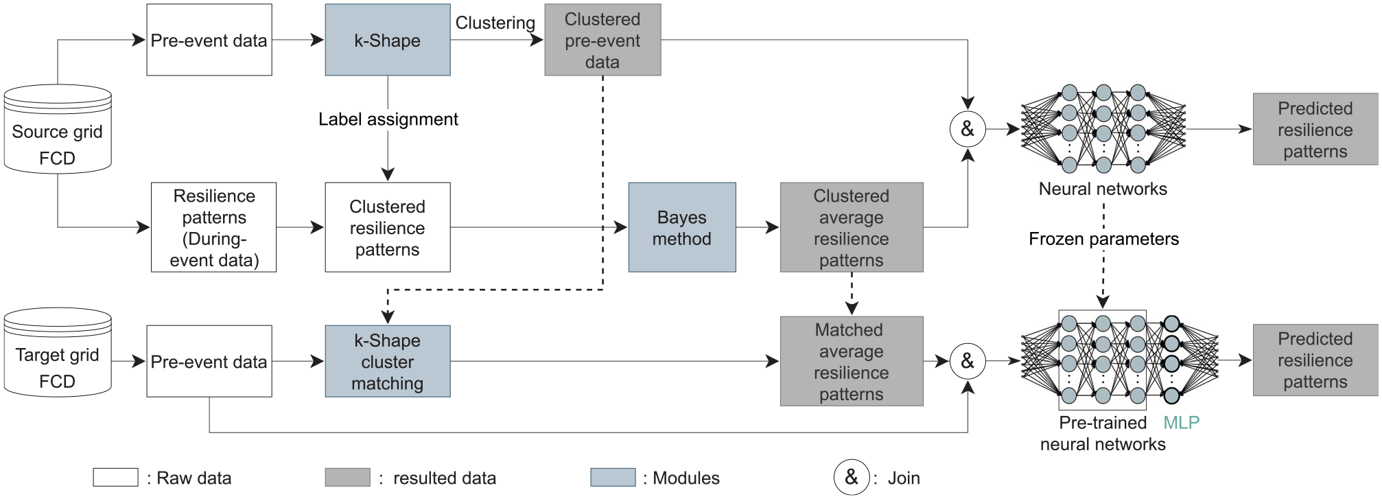
Transfer learning framework for transportation demand resilience prediction.
It is worth noting that the concerned areas/systems require prior division into numerous subsystems in advance, which serve as the unit of analysis in this study. With grid-wise systems as an example, each small system can then be characterized by the respective time series of the traffic volume of floating cars, such as the entering and leaving flows in various directions. These time series will be treated as different observations, recording the development of the functionality of these systems. As such, the time series containing the event period can be used to estimate their resilience patterns in the face of a certain type of event. Although such traffic volume time series vary from city to city, substantial similarities are anticipated among those much smaller grids. Moreover, it is plausible to assume that grids exhibiting similar pre-event characteristics would manifest comparable resilience patterns in similar events. Here, resilience patterns are defined as the changing patterns of the traffic volume time series during the life cycle of the event. In addition, we consider multiple cities in transfer learning models, within which the cities with during-event data are treated as source cities, and otherwise target cities.
To measure the similarities of different grid systems, we applied the k-Shape time series clustering method to cluster the pre-event time series. Note that in this step, the raw grid traffic volume time series from different source cities are mixed and inputted to the k-Shape method. Then, the clusters identified are used to label the corresponding during-event time series. Namely, the resilience patterns of different grid clusters are defined according to their pre-event functionality.
Given the stochastic nature of FCD, extracting the average resilience pattern for each grid cluster is necessary. To this end, we applied the Bayes method for each cluster to infer the posterior distribution of the during-event traffic volume time series. Thus, traffic volume distributions at every time step can be obtained for grids that belong to the same cluster. We denote the mean values of the distributions as the extracted prompt features. The extracted prompt features’ sequence represents each cluster’s average resilience pattern.
As presented in Figure 1, the clustered pre-event time series and their corresponding average resilience patterns are joined together and fed into neural networks to predict the actual resilience patterns. In this way, the pre-trained models are obtained. For the test set, only pre-event data is given. The pre-event data of the test set are first matched to the corresponding cluster identified using the source data. Then, by joining the pre-event data and the average resilience patterns of the matched cluster, one can obtain the same format of input as those used to train the source model. The joined sequences are then fed into the pre-trained neural networks with frozen parameters. Each pre-trained neural network is stacked with a multi-layer perceptron (MLP) for parameter learning. It follows that the transfer learning model can predict the resilience patterns for the target cities with only the pre-event data.
Time Series Clustering
We applied time series clustering to categorize grids with similar pre-event patterns. We denote the traffic volume time series dataset of an n-grid city as
We apply the k-Shape algorithm to identify grids with similar resilience patterns. The k-Shape algorithm is a k-means-based clustering method with shape-based distance (SBD) as the distance measure. Figure 2 illustrates the application of the k-Shape algorithm in this problem. Firstly, the algorithm is implemented on the partition of pre-event time series,
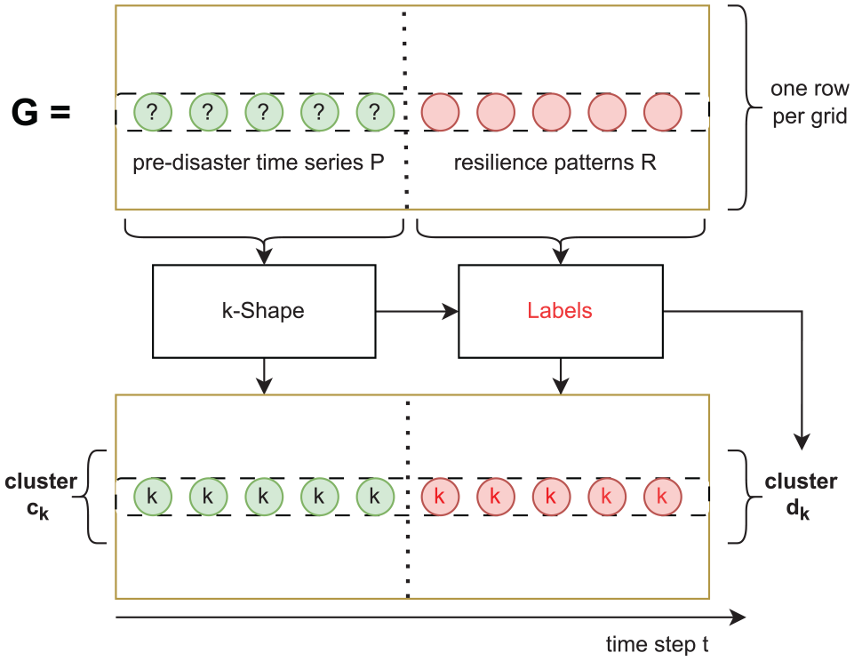
The k-Shape time series clustering for grid floating car data.
Bayes-Based Shape Extractor
Assume that for a resilience pattern cluster
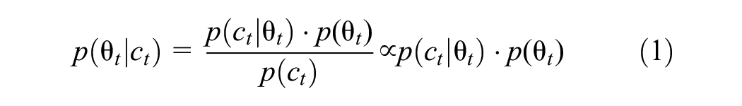
where
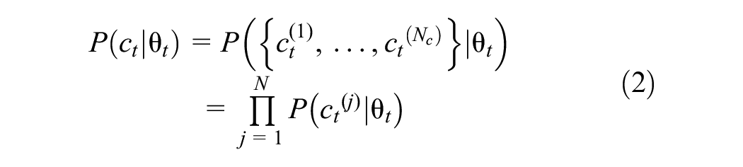
For each time step
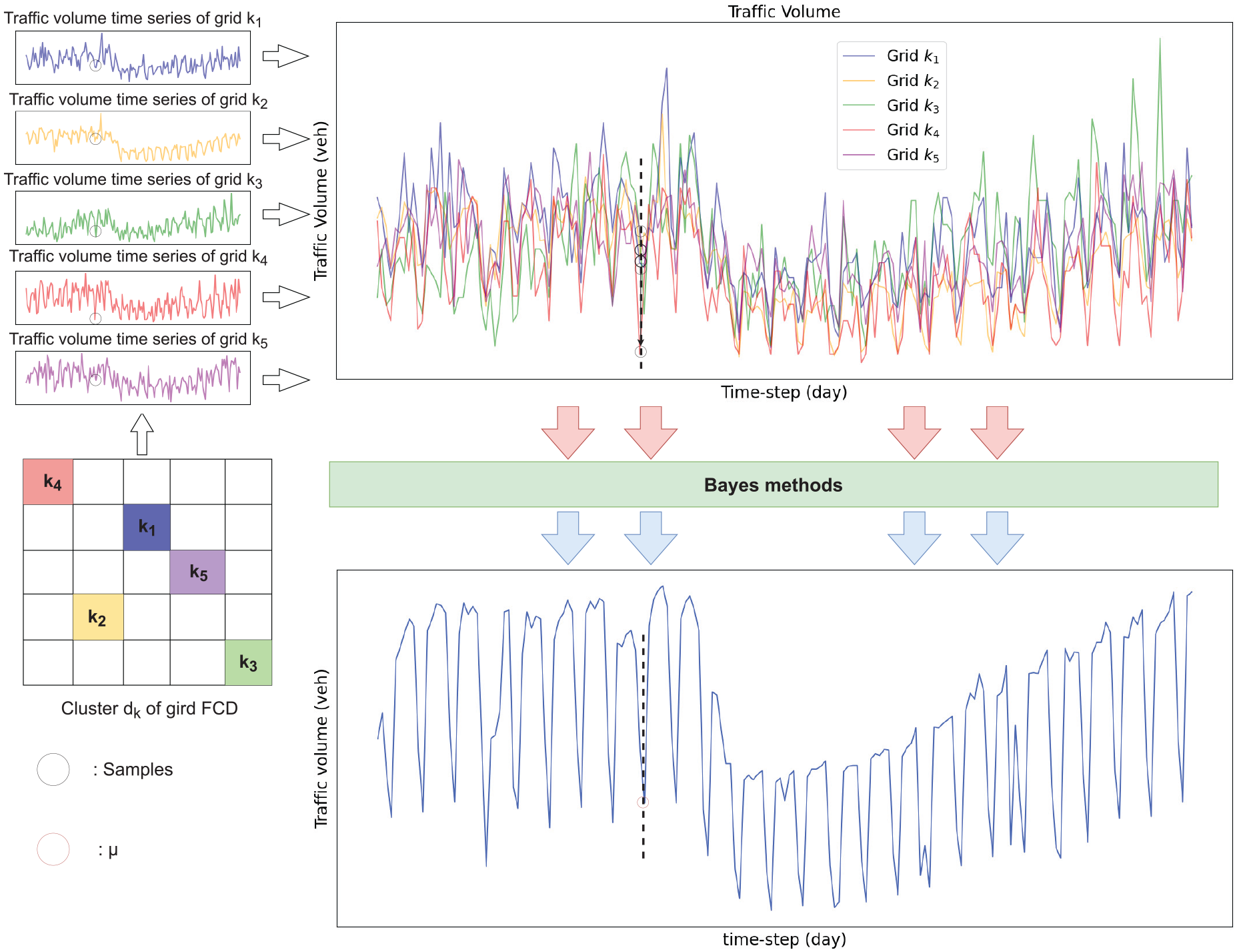
Example of Bayes resilience patterns extraction. Here we mark an example of resilience pattern extraction for a single time step. The samples of each time step form a dataset. For each cluster
Neural Networks
The application of k-Shape clustering and the Bayes method enables the extraction of prior knowledge about resilience patterns, thus enriching the feature set for the transfer learning dataset. To acquire deep embedding of the features and accomplish prediction tasks, deep learning models are applied to learn the model parameters. This study considers two kinds of deep learning models: MLP and RNNs. For RNNs, we consider a conventional RNN and an LSTM network.
Multi-Layer Perceptron
The MLP is a basic type of feed-forward neural network (FNN). The nodes of a FNN are connected in a directed graph without a circular structure. The inputs of a FNN only flow from the input layer through hidden layers to the output layer in one direction. In this study, the inputs of the MLP are the joined sequences comprising the pre-event time series and the corresponding resilience patterns derived by the Bayes method. The outputs are the predicted resilience patterns.
Recurrent Neural Network
In contrast to FNNs, RNNs share parameters across various time steps, enabling the model to handle the variable-length sequence. The RNN model processes one input at a time, and for each layer, the inputs are not only the features of the current time step but also the hidden features from the last time step, thereby enabling the RNN to capture the temporal dependency of the time series. In this study, the inputs of the RNN are also the joined sequences comprising the pre-event time series and the corresponding Bayes resilience patterns. Only the outputs from the last few layers are optimized to predict the resilience patterns.
Long Short-Term Memory
The LSTM is a variant of the RNN, which is designed to solve the gradient problem to capture more information from the past. In the RNN, the outputs can only be optimized through hidden features. Once the weights are smaller than zero or larger than one, based on the backward propagation through time (BPTT) and the chain rule, the successive derivations of the latest outputs can result in their gradients to the previous inputs converging to either zero or infinity when predicting for a long sequence. Therefore, the previous information is challenging to propagate to distant future units. An LSTM unit contains a memory cell, an input gate, a forget gate, and an output gate. The memory cell is introduced to aggregate the past and current information, the flow of which is adjusted by the gate units so that the information can be selectively transmitted to the following LSTM units to keep a long-term temporal dependency.
Case Study
In this section, we introduce the case study for the following experiments, which are conducted in the context of the COVID-19 pandemic. We first analyze the impact of COVID-19 on urban transportation systems. Then, we describe the situation of the study areas and the FCD used in the experiments.
The Impact of COVID-19 on Transportation
Unlike general events, the COVID-19 pandemic did not destroy the transportation infrastructure directly but rather affected travel behaviors and limited the travel opportunities of citizens. To protect the health of citizens and mitigate the economic fallout caused by the pandemic, governments of different countries and regions have taken a series of emergency measures. Among them, the lockdown of event venues, short-term travel control of citizens, and quarantine policies are the most commonly used measures. According to Engle et al. ( 25 ), the mobility of the population is sensitive to the government’s stay-at-home announcement, which alters travel behavior and restricts citizen mobility, thereby substantially reducing traffic demand over a certain period.
Under the pandemic control policies, the traffic volumes of many cities showed a sharp decline and then gradually recovered as the control measures were relaxed. Although “resilience triangles” showed in most of the city road networks, the impact of COVID-19 varied greatly in different cities because of their unique topologies and response policies ( 26 ). Therefore, learning from the experience of other cities and studying how to transfer the knowledge of resilience patterns play essential roles. In the following experiments, we applied the proposed method to the grid traffic volume FCD from three cities: Antwerp, Bangkok, and Barcelona. We used the data of Antwerp and Bangkok for source domain model training and the FCD from Barcelona for transfer learning.
Study Areas
Antwerp is the largest city in Belgium, which is located in the Antwerp Province in the Flemish region. As presented in Figure 4a, the road network of Antwerp has a radial structure with a relatively dense road network in the city center and a sparse road network on the outskirts. To combat the spread of the COVID-19 virus, Belgium implemented lockdown policies on March 18, 2020. The lockdown measures affected schools, restaurants, and workplaces across the entire nation. The traffic volume decreased sharply under the pandemic intervention measures until May 4, 2020, when the lockdown measures were gradually eased, some urban amenities were allowed to reopen, and the traffic volume started to recover.
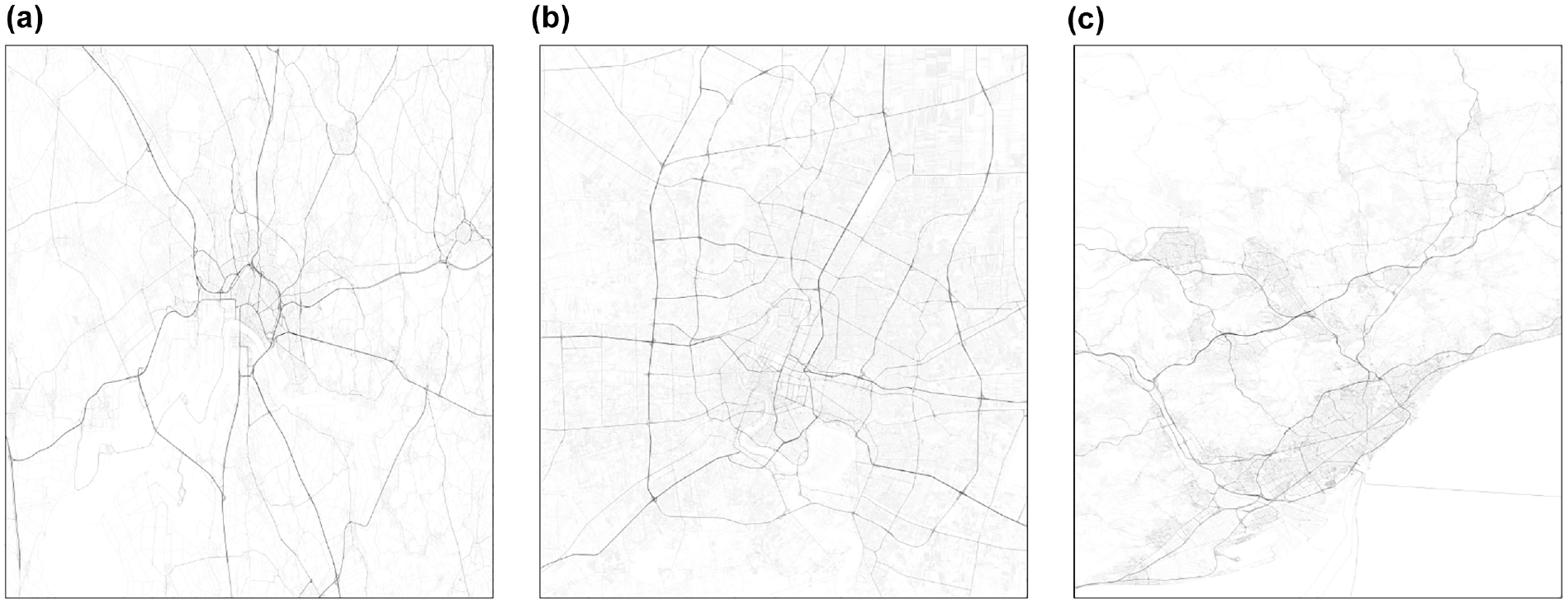
Study areas and networks. (a) Antwerp network. (b) Bangkok network. (c) Barcelona network.
Bangkok, situated in the country’s center, is the capital of Thailand. As presented in Figure 4b, the road network of Bangkok exhibits a ring structure, with the roads within the ring demonstrating a mix of grid and radial layouts. The pandemic intervention measures in Bangkok were initiated on January 3, 2020, when the Thai Ministry of Public Health started to screen the temperature and issue health declaration cards to travelers. From March 3, 2020, the Thai government commenced prohibitions on large gatherings and closures of schools and entertainment venues. Shortly after the closures, the government imposed a curfew from March 26 to May 17, 2020, when entertainment places were allowed to reopen. Because of the timely implementation of pandemic intervention policies, the transportation system of the Bangkok road network was relatively less affected by the pandemic and showed more resilient patterns.
Barcelona, the city for the transfer learning experiment in this study, is located on the northeast coast of Spain. As presented in Figure 4c, Barcelona has a comprehensive network structure that consists mainly of ring and radial roads, and some blocks in the city center have a grid structure. The government of Spain implemented lockdown measures on March 14, 2020, and extended the measures until April, 26. Following that, the prevention measures began to ease, and on May 11, 2020, citizens were incrementally permitted to resume social activities. During the pandemic, the traffic volume in Barcelona experienced a sharp decline and then gradually recovered at an unstable rate.
Floating Car Data Description
The grid traffic volume FCD is provided by HERE ( 27 ) and was used for NeurIPS Traffic4cast competitions ( 28 ). The data from each city is split into two halves: the first half, ranging from January 2, 2019, to June 30, 2019, before the COVID pandemic, and the second half from January 2, 2020, to June 30, 2020, during the first outbreak of the pandemic. Therefore, the data contains 180 days of pre-COVID patterns and 181 days during and after the first outbreak patterns. As shown in Figure 5, the raw data for our experiment is a (288, 495, 436, 4) tensor for one day. The first three dimensions encode the number of 5-min time intervals per day and the number of 100 m × 100 m grids for each city, and the four channels encode the traffic volume of four different directions of each grid. In our experiment, we merged the time interval into one day to avoid multiple seasonality.
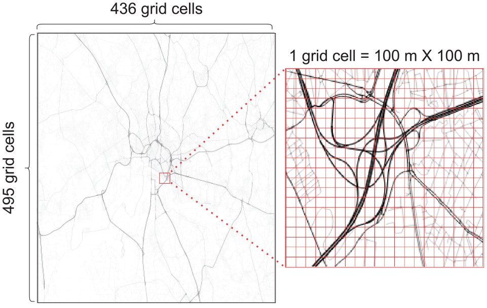
Grid floating car data.
Experimental Design
Data Preprocessing
Since the spatial partitioning of the raw data is based on image pixels rather than the road network structure, grids without roads typically do not contain traffic volume, and grids with small traffic volume exhibit unstable trends in time series. Consequently, data preprocessing was conducted to remove the grids where traffic volume was either unavailable or abnormal.
Data preprocessing involves the following steps: (1) aggregating the traffic volume into one-day intervals; (2) folding the data into four dimensions (cities, total samples of four directions, time steps, traffic volume); (3) setting a threshold to eliminate part of the abnormal data, that is, the average traffic volume per day of each grid should be greater than
We first pre-trained the neural networks using the 180-day pre-pandemic FCD traffic volume for the source domain cities to predict the 181-day resilience patterns. Then, the pre-trained models were fine-tuned to predict 181-day resilience patterns for the target domain with only 50 days of its pre-pandemic data. Therefore, the total input sequence lengths of the source domain and target domain time series are 361 and 231, respectively.
For a 100 m × 100 m grid size, each city contains 495 × 436 grid cells, and each grid contains the traffic volume time series from four different directions, which means that for each city, a maximum of 863,280 traffic volume time series can be extracted. The threshold
Model Evaluation
The architectures of the neural networks are shown in Table 1. We employed the rectified linear unit (ReLU) activation function for more effective learning. The initial learning rate is set to 0.001, and we applied the step decay schedule with the decay rate of 0.75 per 50 steps. The batch size for all models is taken as 64.
Model Architecture
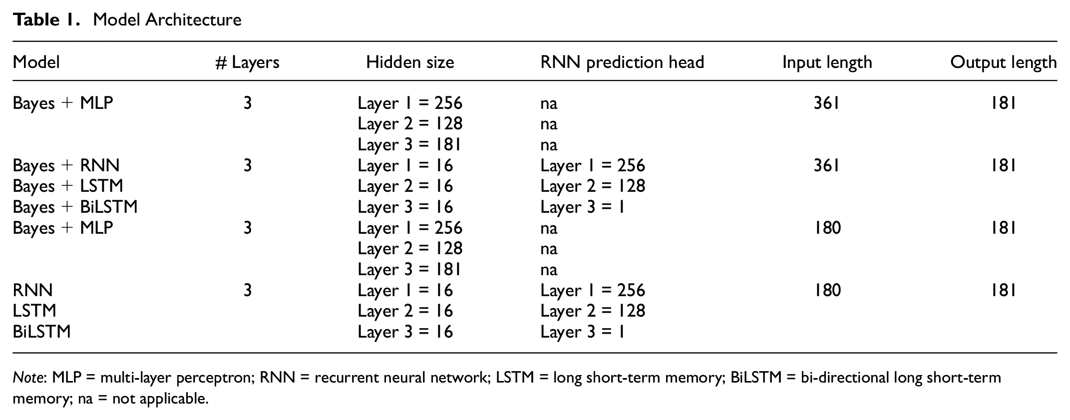
Note: MLP = multi-layer perceptron; RNN = recurrent neural network; LSTM = long short-term memory; BiLSTM = bi-directional long short-term memory; na = not applicable.
Initially, we applied a Bayes patterns extractor to generate the average resilience patterns for each cluster, the sequence length of which is 181. Therefore, the input sequence length of each neural network is the sum of the pre-pandemic sequence length and the average resilience pattern length, which is 361. To demonstrate the effectiveness of the proposed Bayes resilience patterns extractor, we performed an ablation experiment, that is, comparing the case with and without the extractor. Without the extractor, the average resilience patterns in Figure 3 are unable to be extracted, and therefore we directly fed the pre-pandemic sequence into the neural network with the same architecture as our proposed model. For each RNN, we added a feed-forward network as the prediction head to generate the output. For transfer learning, the parameters of all models were frozen, and their outputs were fed into an FNN for fine-tuning.
For model performance evaluation, we employed the mean absolute error (MAE), root-mean-squared error (RMSE), and DTW as metrics, which are defined as follows:


where
Results
Macroscopic Traffic Volume Resilience Patterns
The total traffic volume time series of the three cities are presented in Figures 6–8, respectively. Compared with their pandemic intervention timeline, it can be observed that they have different patterns before and during the pandemic.
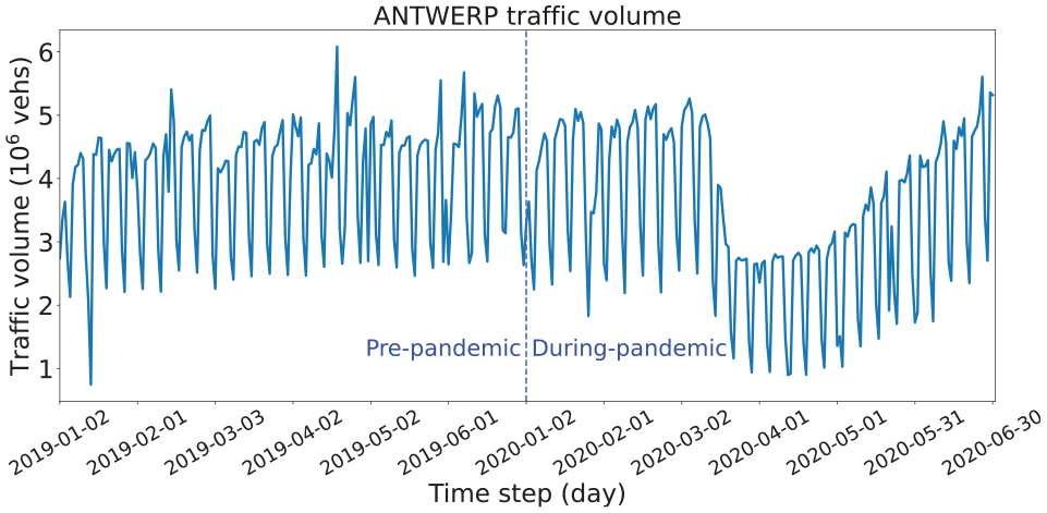
Antwerp traffic volume time series.
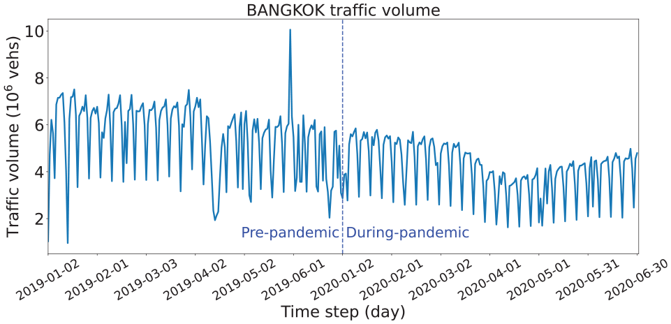
Bangkok traffic volume time series.
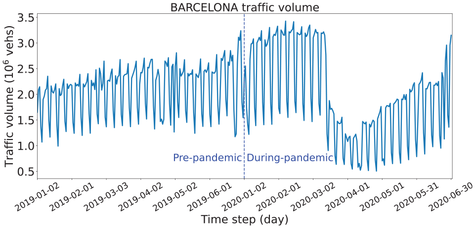
Barcelona traffic volume time series.
As shown in Figure 6, the trend of Antwerp’s traffic volume time series was relatively stable before the pandemic. In the first half year of 2019, the values showed a slightly increasing trend and remained at the same level in the first three months of 2020. Subsequently, the government of Antwerp implemented pandemic preventive measures in March 2020, leading to a sharp decline in traffic flow, reaching its minimum point. It was only half of the pre-pandemic level by the end of March and maintained a low level afterward. As the preventive policies were eased in early May, the traffic volume gradually recovered with a slightly accelerating trend. By the end of June, the overall traffic volume in Antwerp had recovered to its pre-pandemic level.
Figure 7 shows that the traffic volume trend in Bangkok was relatively stable before April 2019, followed by a slight decline. In early 2020, because of the timely prevention measures, the traffic volume had a slightly decreasing trend and declined to the minimum point at the beginning of April. In March 2020, the curve recovered gradually but failed to reach its original state. The traffic volume in Bangkok did not experience a sharp decrease during the pandemic. Instead, it exhibited an overall decreasing trend.
Figure 8 shows the traffic volume patterns in Barcelona. Unlike the previous two cities, its traffic volume increased gradually before 2020 and was relatively stable in early 2020. Then a plunge showed in the curve because of the implementation of the lockdown policies in March and remained at a low level. After the lockdown, the traffic volume trended upward and recovered to the pre-pandemic level.
From the macro level, the overall traffic volume in each of the three cities has distinct trends and resilience patterns. However, from a microscopic view, the grids of each city contain various patterns, and for different cities, some of their grids may contain the same patterns.
Results of the Source Domain Model
Average Resilience Patterns
We utilize the elbow method to determine the optimal number of clusters. The elbow method plots the within-cluster sum of squares (WCSS) against the number of clusters. The WCSS represents the total squared distance between each point and the centroid within its cluster, and the point of inflection on the WCSS curve, often referred to as the “elbow,” is selected as the number of clusters.
Based on the WCSS curve given in Figure 9, the number of clusters can either be set to three or four. Although more clusters could lead to high inter-cluster similarities, the pre-pandemic time series were segmented into four clusters by the k-Shape method for extracting more resilience patterns. Figure 10 presents each cluster’s clustering centroids of the pre-pandemic time series. To verify our assumption presented in the Methodology section that grids exhibiting similar pre-event patterns would manifest comparable resilience patterns in the face of similar events, the k-Shape method was also applied to the entire traffic volume time series, which includes both pre-pandemic and during-pandemic time series. The grids within the clusters that were generated based on the entire time series have high similarity across the entire time series, and the pre-pandemic part of these also exhibited high similarities with the clustering centroids generated by using only the pre-pandemic time series, except cluster 0. This validates our assumption. According to Paparrizos and Gravano ( 24 ), the cluster centroid is computed by maximizing the cross-correlation similarity between a given sequence and the time series within the cluster. Thus, the cluster centroid intuitively reflects the time series shape within the cluster. Note that the magnitude deviation is caused by normalization, and the offset in the time dimension does not affect the clustering results as the k-Shape method aligned the time series automatically when calculating the SBD between time series. Figure 10, a and b , shows that the first two clusters comprised the normalized traffic volume pre-pandemic time series with overall stable trends. The centroid of cluster 0 shows smaller amplitudes and some unstable amplitudes, and the reason is that cluster 0 captured more grids containing smaller traffic volumes, which generally exhibit less stable trends, but the fluctuations are limited in range. On the other hand, the centroids of the last two clusters each exhibit different declining trends at different time steps. In addition, the centroid of each cluster shows similar seasonality and amplitudes through time, which means the elements within the same cluster have high similarity.
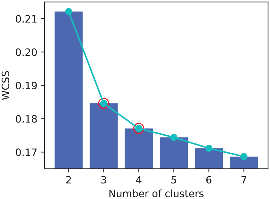
Within-cluster sum of squares (WCSS) of different numbers of clusters.
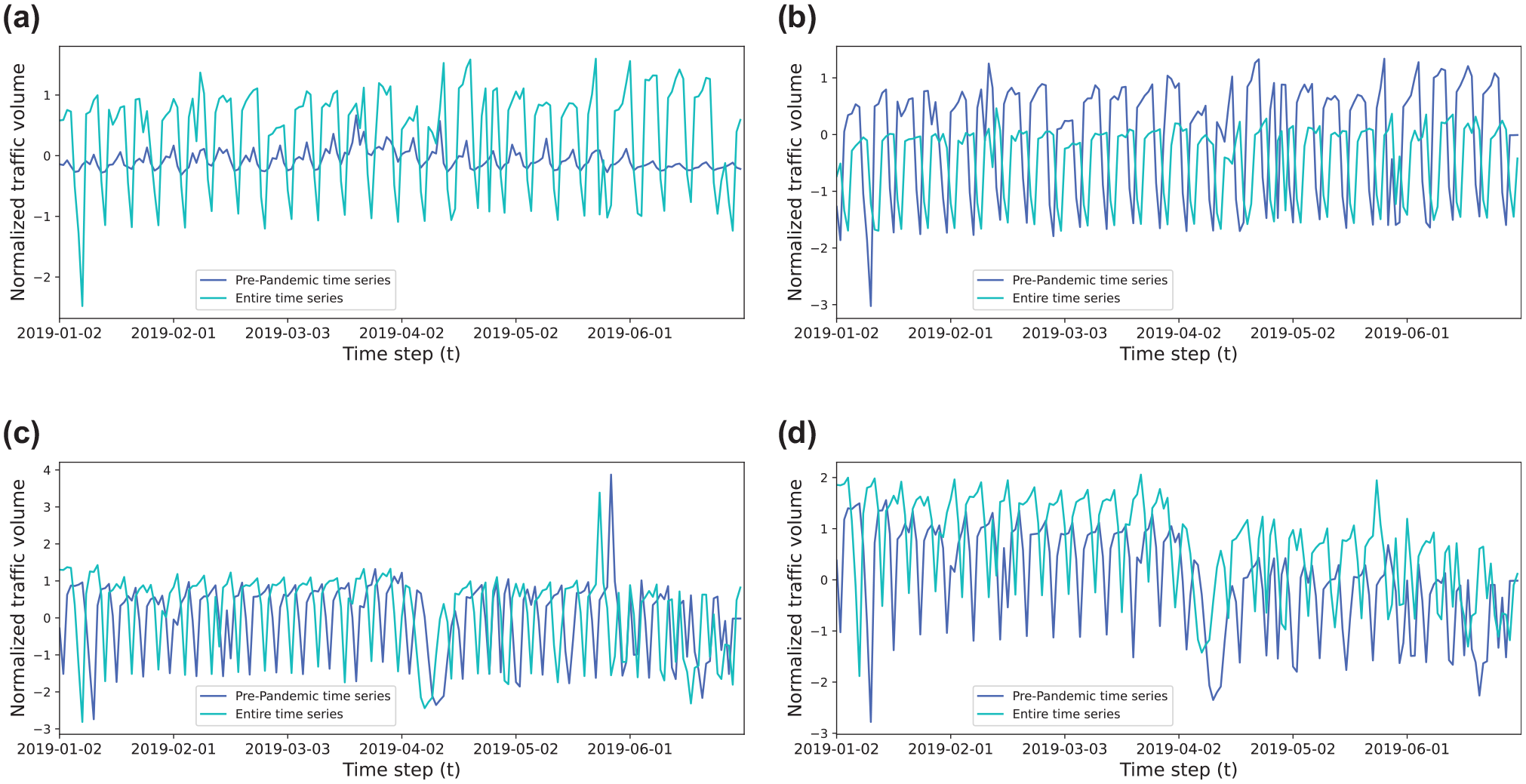
Clustering centers of pre-pandemic clusters. (a) Cluster 0 (pre-disaster). (b) Cluster 1 (pre-disaster). (c) Cluster 2 (pre-disaster). (d) Cluster 3 (pre-disaster).
According to the clustering results of the pre-pandemic time series, the resilience patterns can likewise be segmented into four clusters. Figure 11 presents the samples of during-pandemic time series and the extracted average resilience patterns from all elements in each cluster. Consistent with pre-pandemic clusters, an apparent bolded trend curve can also be observed among the samples of each cluster. The average resilience patterns reflect the possible normalized traffic volume with the highest degree of confidence in each cluster. As shown in Figure 11a, the average resilience pattern of cluster 0 showed a slightly downward trend in mid-March 2020 and a slow upward trend since April 2020. In contrast, the average resilience pattern of cluster 1 (see Figure 11b) presented a more distinct “resilience triangle” shape. The extracted time series in Figure 11, c, and d had an overall downward trend and slight resilience patterns.
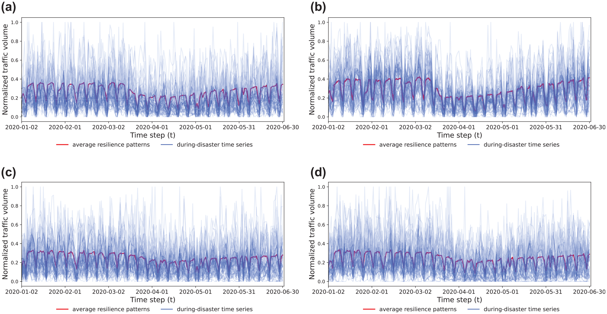
During-pandemic clusters and average resilience patterns. (a) Resilience patterns of cluster 0. (b) Resilience patterns of cluster 1. (c) Resilience patterns of cluster 2. (d) Resilience patterns of cluster 3.
Results of Neural Networks
Table 2 summarizes the performance of different models under different metrics when predicting traffic volume resilience patterns at the grid level.
Source Domain Ablation Experiment
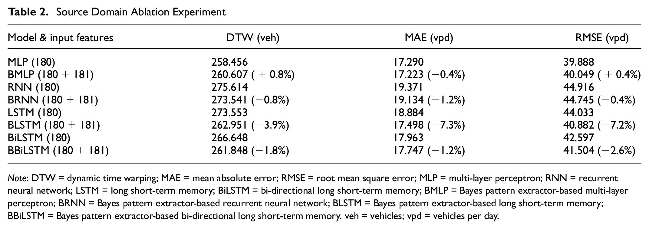
Note: DTW = dynamic time warping; MAE = mean absolute error; RMSE = root mean square error; MLP = multi-layer perceptron; RNN = recurrent neural network; LSTM = long short-term memory; BiLSTM = bi-directional long short-term memory; BMLP = Bayes pattern extractor-based multi-layer perceptron; BRNN = Bayes pattern extractor-based recurrent neural network; BLSTM = Bayes pattern extractor-based long short-term memory; BBiLSTM = Bayes pattern extractor-based bi-directional long short-term memory. veh = vehicles; vpd = vehicles per day.
In the source domain, it is unequivocally demonstrated that the MLP model underpinned by a Bayes patterns extractor (BMLP) exhibits superior performance across all three metrics. In contrast, the Bayes pattern extractor-based RNN (BRNN) model performed worst. Both the LSTM model and the bi-directional long short-term memory (BiLSTM) model, equipped with Bayes pattern extractors (BLSTM and BBiLSTM, respectively), demonstrated comparable performance to the BMLP. For DTW, the performance of the BMLP, BLSTM, and BBiLSTM was almost identical, while the performance of the BRNN was worse. Apparently, the BRNN model failed to capture the similarity of the traffic volume time series. For the MAE, the BLSTM and BBiLSTM models achieved similar performance to the BMLP model, while the MAE of the BRNN model was significantly lower than that of the other models, indicating its relatively poor prediction accuracy. With respect to the RMSE, the BMLP and BLSTM models had relatively low values of around 40, significantly lower than the value of the BRNN model. The recorded RMSE values show that significant errors less influenced the predictions of the BMLP and BLSTM models compared to the BiLSTM and BRNN models.
Moreover, it can be observed that the resilience patterns extracted by the Bayes patterns extractor can improve the overall performance of RNN-based models but fail to improve the performance of the MLP. However, in RNN-based models, the improvement of the BRNN compared to the traditional RNN was marginal. In contrast, both the BLSTM and BBiLSTM significantly outperformed the LSTM and BiLSTM across all measured metrics. A possible explanation for this could be that the memory capability of the RNN for pre-pandemic information is inferior to those of the LSTM and BiLSTM over longer prediction lengths.
It can be noticed that the BMLP model exhibited more robust prediction performance than RNN-based models in the source domain. The possible reason could be the cumulative error caused by the long prediction length. In RNN-based models, the BLSTM and BiLSTM outperformed the BRNN because the gate mechanism can strengthen the ability of the LTSM-based model to capture the long-term temporal dependencies, thereby achieving similar performance to the BMLP model.
Figure 12 presents the performance of the proposed models as well as the Bayes ablated models. It can be observed that the predictions of the Bayes-based model are almost consistent with the ground truth. As shown in Figure 12a, the BMLP exhibited strong robustness over the entire forecasting interval, but a noticeable bias is evident when predicting the peak value for the initial month. In addition, it possessed relatively low precision at the time steps marked by substantial changes in trends, which indicates that the BMLP struggled to capture the dependency between adjacent time steps but can learn the overall shape of the resilience patterns. On the other hand, Figure 12b illustrates that the BRNN performs well in the prediction from January to March but fails to predict accurately during April and May when clear frustration presents. This implies that the BRNN has limitations in capturing the long-term dependencies of the sequence and is not sensitive enough to the changes in the trends of the time series. The BLSTM model was relatively robust throughout the entire prediction interval, as displayed in Figure 12c. Compared to the BMLP, the BLSTM performs better in peak values and is also capable of capturing significant changes in trends. However, the BLSTM is unstable in predicting the valley values of each period in our experiment. As shown in Figure 12d, the BBiLSTM performs better in predicting peak-to-peak values in the first few months. However, for the prediction from mid-March to the end of May, the BiLSTM continuously overestimated the traffic volume.
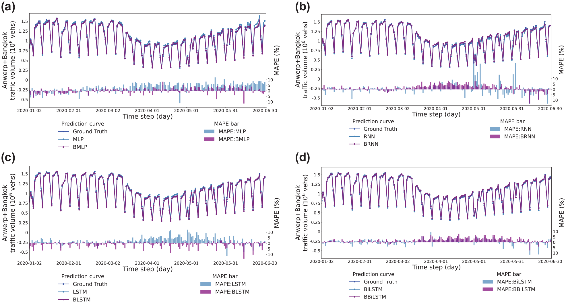
The macro-level prediction and true values in the source domain. (a) Multi-layer perceptron (MLP) model. (b) Recurrent neural network (RNN) model. (c) Long short-term memory (LSTM) model. (d) Bi-directional long short-term memory (BiLSTM) model.
To quantify and compare the performance of different models in different experiments for the macro-level prediction, we further introduced the MAPE as the metric. The bar charts of Figure 12 present the MAPE of different neural networks for each time step.
Results of the Target Domain Model
In the target domain, the input was only 50 days of the Barcelona pre-pandemic traffic volume time series, and an FNN was stacked to each pre-trained model for fine-tuning. Table 3 lists the prediction performance comparison of different models under different metrics at the grid level.
Target Domain Ablation Experiment
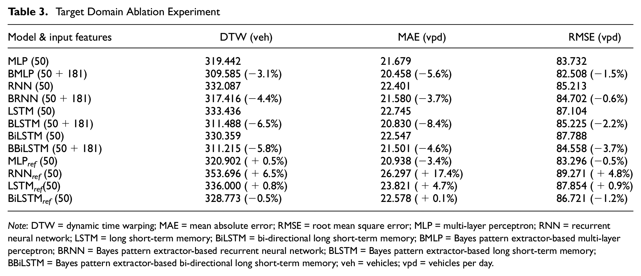
Note: DTW = dynamic time warping; MAE = mean absolute error; RMSE = root mean square error; MLP = multi-layer perceptron; RNN = recurrent neural network; LSTM = long short-term memory; BiLSTM = bi-directional long short-term memory; BMLP = Bayes pattern extractor-based multi-layer perceptron; BRNN = Bayes pattern extractor-based recurrent neural network; BLSTM = Bayes pattern extractor-based long short-term memory; BBiLSTM = Bayes pattern extractor-based bi-directional long short-term memory; veh = vehicles; vpd = vehicles per day.
In general, similar to the results of the source domain models, the BMLP showed the strongest robustness across all three metrics, whereas the BRNN delivered the poorest performance. The BLSTM and BBiLSTM exhibited similar performance. The DTW results were consistent between the target and source domains. The BMLP-based transfer learning model continued to exhibit the most prominent performance in capturing the similarity between traffic volume time series. The BLSTM and BBiLSTM exhibited comparable DTW performances, which were close to that of the BMLP. However, the BRNN still performed poorly in learning time series similarity. The MAE results show that the BLSTM and BMLP achieved high accuracy in our traffic volume prediction task, while the BBiLSTM and BRNN had approximately 4% lower prediction accuracy. With respect to the RMSE, the BMLP yielded significantly lower errors than other models. Although the BLSTM exhibited the highest accuracy in MAE error, the BBiLSTM and BRNN models were less affected by significant errors.
Compared to the source domain tasks, the performance of the BRNN was closer to that of other models. In the source domain, the performance of the BRNN and other models differs by approximately 5% with respect to the DTW metric. However, in the transfer learning experiment, the gap had reduced to approximately 2%–2.5%. With respect to the MAE, the performance of the BRNN was even closer to the BBiLSTM and exhibited better performance than in the source domain. With respect to the RMSE, the BRNN’s performance surpassed that of the BLSTM and was close to that of the BBiLSTM. This result suggests that although RNN models have a relatively poor ability to capture the similarity of traffic volume time series at the micro level, they exhibited good generalization ability in predictive accuracy.
Moreover, the proposed models showed stronger robustness in transfer learning. Compared to the Bayes component ablated models for DTW, the BMLP, BRNN, BLSTM, and BBiLSTM models performed more robustly in capturing time series similarity by 3.1%, 4.4%, 6.5%, and 5.8%, respectively. The accuracy of the proposed models also improved by 5.6%, 3.7%, 8.4%, and 4.6% with respect to the MAE. Moreover, for the RMSE, the accuracy of our models increased by 0.6% to 3.7%.
From a macro perspective, all four models achieved robust prediction performance for relatively stable trends but exhibited particular bias in predicting the valleys of the overall resilience pattern, as shown in the line charts of Figure 13. Figure 13a illustrates the prediction results of the BMLP model in the target domain. It can be observed that the BMLP model delivered a generally robust performance, particularly during periods with significant trend changes. Figure 13b shows that although the BRNN model could capture the overall trend of the time series, its predictive ability for the valleys of the resilience patterns is limited. Compared to the BRNN model, as shown in Figure 13c, the BLSTM model better captured the downward trend of the resilience patterns, although it overestimated the robustness and resourcefulness of the transportation systems. Figure 13d shows the prediction results of the BBiLSTM, which showed a more robust performance in predicting the traffic volume during the recovery phase of the time series than the BLSTM.
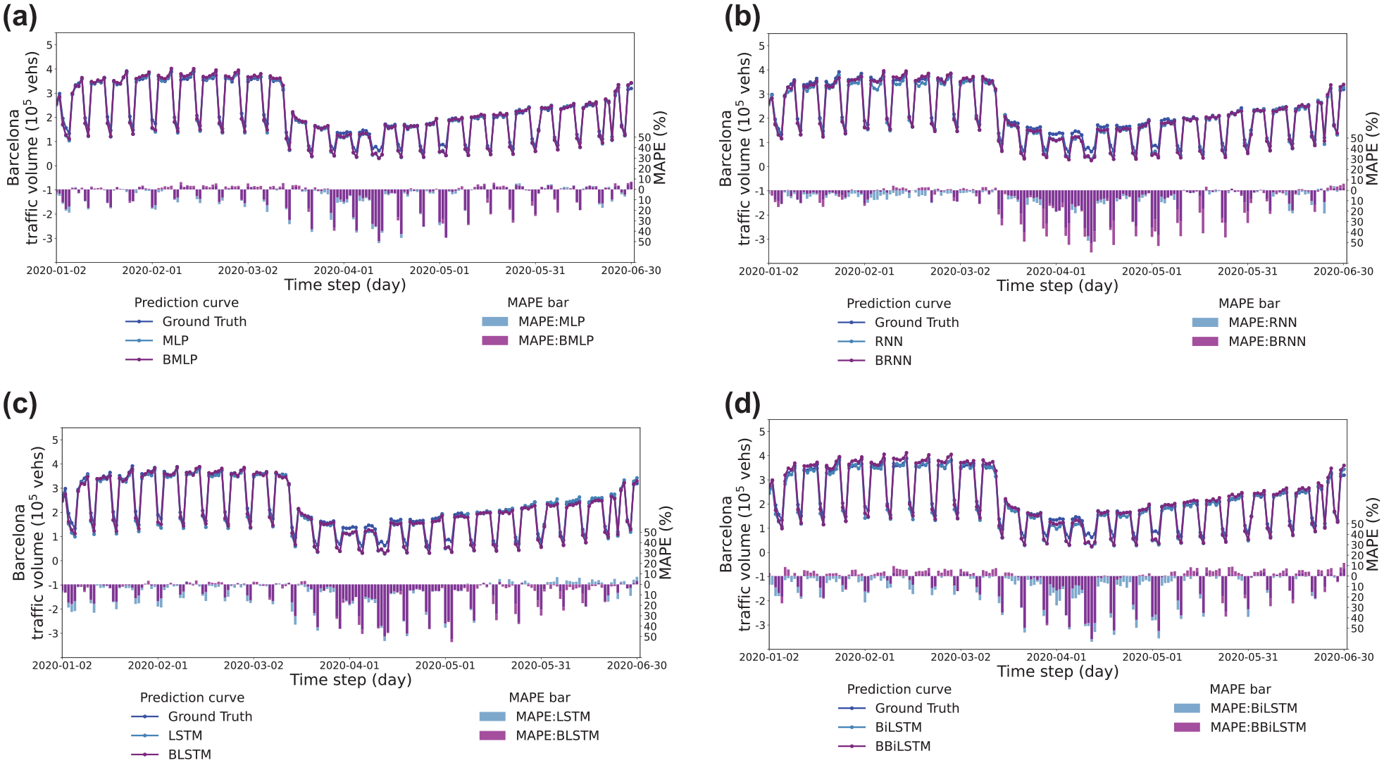
The macro-level prediction and true values in the target domain. (a) Multi-layer perceptron (MLP) model. (b) Recurrent neural network (RNN) model. (c) Long short-term memory (LSTM) model. (d) Bi-directional long short-term memory (BiLSTM) model.
However, Figure 13 suggests that all models experienced large MAPE when the traffic volume was relatively low. Because of the inconsistency of traffic volume distribution between the source domain cities and Barcelona, as well as data instability arising from the small grid size, the models may show subpar prediction performance for the grids and periods characterized by low traffic volumes.
From the ablation experiments, it can be inferred that Bayes pattern extractor-based models primarily contributed to the model’s robustness in predicting peak and valley values. Although the Bayes component ablated models (MLP, RNN, LSTM, BiLSTM) could learn temporal dependencies between different patterns, they all continuously overestimated or underestimated the traffic volume in predicting the overall city resilience patterns. The reason could be the over-capturing of the local unstable traffic trends, which made them fail to express the global traffic volume trends. In long-term prediction tasks, the accumulative error also was a limitation for RNN-based models (RNN, LSTM, and BiLSTM). However, introducing the Bayes pattern extractor can provide global information to the neural networks and make the input grid time series more stable, which could enhance the models’ robustness in predicting the overall traffic volume at the macro level. On the other hand, the quality of traffic volume FCD is highly contingent on the number of vehicles connected, which can increase the instability of data with a small grid size. However, the extracted resilience patterns might prevent the models from learning such unstable trends. Therefore, some models did not show significant improvements at the grid level.
Effectiveness of Transfer Learning
The bottom partition of Table 3 shows the performance of transfer learning by comparing the neural networks trained directly (MLP ref , RNN ref , LSTM ref , BiLSTM ref ) and those trained by transfer learning.
The input of all neural networks was the time series with only a 50-day pre-event traffic volume. While transfer learning improved the performance of most models, it led to lower predicted performance for the MLP and BiLSTM, which indicates a negative transfer issue. For the RNN and LSTM, the predicted performance of all metrics was improved by transfer learning, and the improvement of the RNN was particularly significant, as the RNN is less robust and more sensitive to data scarcity. In contrast, the LSTM benefited only marginally from transfer learning. In addition, Table 3 demonstrates that all neural networks supported by the Bayes resilience patterns extractor outperformed both Bayes component ablated models and models trained directly, which evidences that the proposed transfer learning strategy not only enhances the robustness of neural networks but also mitigates the negative transfer problem.
Conclusions
This study built a transferable model for capturing and predicting transportation demand resilience patterns using FCD. The framework integrates an unsupervised resilience patterns extractor and different kinds of neural networks. By conducting a case study under the context of the COVID-19 pandemic, we demonstrated the effectiveness of our model.
We applied grid traffic volume as model inputs and sought to capture the transportation resilience patterns. The proposed framework combines unsupervised machine learning methods and supervised deep learning methods. The unsupervised machine learning methods include time series clustering and Bayes inference methods. We developed prompt features for grid-wise systems with homogeneous resilience patterns and derived the average resilience patterns as an additional input to the neural networks. In addition, the average resilience patterns enable the models to learn the experience from other systems. Unlike the existing literature, in which the inputs to models for resilience pattern prediction are mostly the traffic data at the local level or only the macro-level data, we augmented the feature set by incorporating the extracted resilience patterns from different cities, providing macro-level information for the deep learning models. More importantly, we explored and analyzed the performance and transferability of the models with diverse neural network components.
Despite the satisfactory performance of our proposed method in the case study, certain limitations persist. The extracted resilience patterns enabled the proposed method to learn experiences from different grids and cities. However, the COVID-19 pandemic lasted for a relatively consistent duration globally. Consequently, the effectiveness of the proposed method across time series with varying event durations remains unproven. In reality, most events have different durations, and collecting data with the same event duration requires considerable effort and is not always applicable. Besides, the proposed framework relies on the widespread availability of FCD, but the sparsity of the data or the necessity to quantify system resilience using other indicators could lead to more efforts in data collection and exploration of the temporal characteristics of different indicators. We assumed cities with similar pre-event traffic volume patterns would exhibit similar resilience patterns during the pandemic. Therefore, we applied time series clustering to capture the similarity between grids. However, the performance of time series clustering depends on how similar the pre-event patterns between different grids and cities are. In this study, we only used the FCD from two cities for resilience patterns extraction, which could not guarantee that each grid from the target city could have the right category to correspond. In addition, because of the variability in socioeconomic resources and event response measures among different cities, the reaction of citizens from different cities to large events could be different, even if they have similar driving patterns. Therefore, the proposed method should be more predictive within a single country or region. Furthermore, this paper only considered the similarity of the data itself but neglected the spatial similarity between grids. Therefore, introducing spatial features could potentially enhance grid clustering and accuracy in resilience pattern extraction.
Footnotes
Author Contributions
The authors confirm contribution to the paper as follows: study conception and design: N. Yang, Q.-L. Lu, C. Lyu, C. Antoniou; data collection: N. Yang, Q.-L. Lu; analysis and interpretation of results: N. Yang, Q.-L. Lu, C. Lyu; draft manuscript preparation: N. Yang, Q.-L. Lu, C. Lyu, C. Antoniou. All authors reviewed the results and approved the final version of the manuscript.
Declaration of Conflicting Interests
The author(s) declared no potential conflicts of interest with respect to the research, authorship, and/or publication of this article.
Funding
The author(s) disclosed receipt of the following financial support for the research, authorship, and/or publication of this article: This work was supported by the European Interest Group CONCERT-Japan DARUMA project (Grant Number: 01DR21010), funded by the German Federal Ministry of Education and Research (BMBF). This research was also partially funded by the German Federal Ministry for Economic Affairs and Climate Action (BMWK) (PANAMERA project, Grant Number: 19I21016F) and the International Graduate School of Science and Engineering (IGSSE) of the Technical University of Munich (TUM) (MODA project).