
Abstract
Desired speed or free speed distributions are important input parameters for microscopic traffic flow simulations. Whereas driven speeds can be measured, desired speeds are not detectable for all vehicles because of vehicles constraining each other. An established approach to estimating desired speed distributions is the modified Kaplan–Meier approach, which estimates desired speed distributions based on single vehicle data from stationary detectors. We propose a novel approach to determine desired speeds based on vehicle trajectory data. The proposed approach, as well as the modified Kaplan–Meier approach, is applied to a trajectory dataset recorded on a German freeway. With the modified Kaplan–Meier approach, we observed that the resulting desired speed distributions vary by approximately 5 km/h depending on the position of the stationary detectors. The desired speed distributions obtained from the trajectory-based approach are approximately 5 to 10 km/h higher than those estimated by the modified Kaplan–Meier approach. This difference in results is probably because the trajectory-based approach observes each vehicle over a longer distance rather than just at stationary points. Nevertheless, it can be concluded that the estimation of desired speed distributions is subject to a certain degree of inaccuracy. The analysis of the vehicle trajectory data revealed a notable intra-vehicle instability in desired speeds, with a difference of 5 to 7 km/h observed for 40% of the vehicles between different periods of free driving. These findings should be considered in the context of calibrating microscopic traffic flow simulations.
Keywords
The term “desired speed” (or “free speed”) refers to the maximum speed a driver intends to reach. If necessary, the driver performs a lane change to overtake preceding vehicles traveling at lower speeds. The desired speed is individual to each driver, resulting in a distribution of desired speeds across the collective of drivers on a particular road segment. Whereas driven speeds can be measured, desired speeds are not detectable for all vehicles. The relation between driven speed and desired speed can only be assumed for vehicles that are moving freely without being constrained by preceding vehicles. As traffic density increases, the interaction between road users intensifies, leading to fewer freely moving vehicles and consequently a greater disparity between desired and driven speeds. Furthermore, road users with higher desired speeds exhibit a higher likelihood of being constrained compared with those with lower desired speeds ( 1 ). Relying solely on free speeds of a subset of vehicles to infer the desired speed distribution for all road users would result in a systematic underrepresentation of high desired speeds. However, this approach is used in certain studies to determine desired speeds on highways ( 2 , 3 ). The most established method for estimating desired speed distributions is the modified Kaplan–Meier approach ( 4 , 5 ). This approach can be applied to single vehicle data recorded by stationary detectors, consisting of both constrained and unconstrained vehicles.
Desired speed distributions serve as an input parameter for microscopic traffic flow simulations and significantly influence the traffic dynamics within the simulation. Numerical simulations conducted by Lipshtat indicate that the width of the distribution has a significant impact on the stability of traffic flow because it leads to larger variations in desired speeds among individual drivers ( 6 ). These differences result in more drivers being constrained by those with lower desired speeds, inevitably leading to an increased amount of overtaking attempts. Additionally, Farzaneh and Rakha have found that the desired speed distribution also influences the speed at capacity and, therefore, the shape of the fundamental diagram ( 7 ). Thus, it is crucial to calibrate the desired speed distributions in microscopic traffic flow models.
The advancements in drone technology and automatic image processing now offer the possibility to record and analyze vehicle trajectories for traffic flow investigations. Utilizing vehicle trajectories to estimate desired speeds provides significant benefits because it enables the examination of each vehicle over an extended distance. Moreover, it provides flexibility in recording as vehicle trajectories can be captured at almost any desired location, while stationary detectors for recording single vehicle data need to be installed along the observed road segment.
Within the scope of this study, we propose a method to determine desired speed distributions based on vehicle trajectory data. The approach entails identifying intervals within each trajectory where the vehicle travels at free speed. Our evaluations are based on a vehicle trajectory dataset of a 1,200-m-long segment of a German freeway. To examine the validity of the proposed method, we apply the established modified Kaplan–Meier approach to the dataset by synthesizing stationary detector data from the vehicle trajectories. Further, the intra-vehicle stability of desired speed and the overall concept of one global desired speed per vehicle are discussed. To the best of our knowledge, there are currently no published approaches for determining desired speeds from trajectory data.
Literature Review
Desired Speed Estimation
Approaches for estimating desired speed distributions described in the literature are based on product-limit methods. One commonly used method is the estimator by Kaplan and Meier, originally applied in the context of clinical studies ( 8 ). This method features the estimation of survival probabilities over a specific time period, for example, after an operation. Some patients pass away at a specific point in time after the operation because of post-operative complications. Other patients experience different causes of death or drop out of the study. Therefore, all observed lifetimes contribute to the estimation as either a death event or a loss, forming an incomplete observation. The Kaplan–Meier approach is a non-parametric approach, meaning that the resulting distribution does not conform to a specific mathematical function type.
In traffic engineering, desired speed distributions draw an analogy to survival probabilities in medicine. Instead of a time period, we consider speeds, and instead of the events of death and loss, we consider whether a vehicle is unconstrained (free driving) or constrained by preceding vehicles. In the context of desired speeds, the application of the Kaplan–Meier approach was initially introduced by Botma ( 1 ). Hoogendoorn ( 4 , 9 ) and Geistefeldt ( 5 , 10 ) have further developed this approach for estimating desired speeds. In addition, the Kaplan–Meier approach is used in traffic flow analysis to determine distribution functions of freeway capacity ( 10 – 12 ). Also analogous to survival probabilities in medicine, the procedure involves estimating the survival probability of the traffic flow, whereby the capacity represents the lifetime of the traffic flow.
To estimate desired speed distributions, individual vehicle data from stationary detector recordings are used. For each vehicle j passing through the stationary detector, the speed
A significant disadvantage of the Kaplan–Meier approach is that the resulting desired speed distribution strongly depends on the chosen threshold value of the headway. Thus, Hoogendoorn (
4
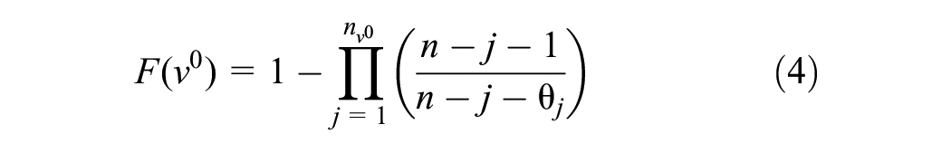
) further developed the Kaplan–Meier approach by including partially constrained observations to the classification as constrained and unconstrained observations. For this modified Kaplan–Meier approach, the probability

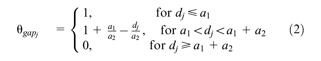
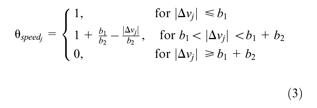
where
In this study, Equation 4, as proposed by Hoogendoorn, is utilized for the modified Kaplan–Meier approach for highways ( 9 ).
where
Trajectory Data in the Context of Microscopic Traffic Simulation
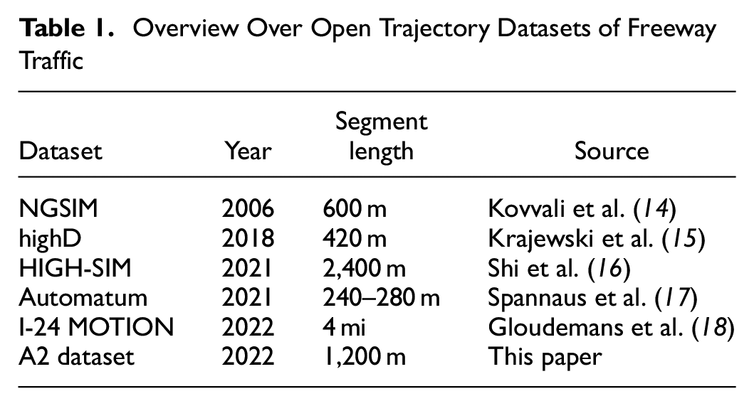
Driven by technological advances in the development of camera drones and automatic image processing, various freely available trajectory datasets have been collected and processed to support the development of trajectory processing and the use of trajectories in the context of simulation models. Table 1 shows a selection of currently available datasets. Research has been conducted on subjects such as traffic flow analysis and modeling, traffic-related estimation and prediction, traffic flow model calibration, vehicle trajectory data cleaning, and vehicular ad hoc network-related studies based on the NGSIM dataset ( 13 ).
Overview Over Open Trajectory Datasets of Freeway Traffic
Hamdar et al. ( 19 ) and Hao et al. ( 20 ) calibrated and validated their proposed car-following models based on trajectories of the NGSIM dataset by comparing speed, acceleration, time headway, and space headway. Przybyla et al. ( 21 ) analyzed trajectories to identify driver behavior and characteristics to propose a data-driven car-following model, whereas Li et al. ( 22 ) examined the distribution of headways collected from NGSIM trajectories. To calibrate Wiedemann’s car-following model in PTV Vissim, Durrani et al. estimated the model parameters directly from the NGSIM trajectories ( 23 ). The study showed that vehicle-following behavior is significantly different among various vehicle classes, and recommends setting parameter values as distributions instead of fixed values. Hale et al. propose a method to calibrate a microscopic traffic flow simulation of a freeway segment by comparing and minimizing the difference between observed and simulated trajectories ( 24 ). To ensure comparing sufficiently similar trajectories, both observed and simulated trajectories have been binned into specific groups. Li et al. ( 25 ) and Zhong et al. ( 26 ) propose approaches similar to Hale et al. ( 24 ) to calibrate the intelligent driver model (IDM) with NGSIM trajectories, whereas Kurtc ( 27 ) demonstrated that the IDM is capable of reproducing naturalistic vehicle trajectories based on the highD dataset.
The literature review shows that vehicle trajectories are a suitable data source for the calibration of microscopic traffic flow simulations, but most studies focus on driving behavior. To the best of our knowledge, there are currently no published approaches for determining desired speeds from trajectory data. Nonetheless, the studies mentioned above indicate that trajectory data is capable of providing the required information to estimate desired speeds, such as speed, acceleration, as well as time and space headways to the surrounding vehicles.
Method
Used Data
To estimate desired speeds from vehicle trajectories, it is beneficial to have a trajectory dataset with wide spatial coverage. As the length of the recorded trajectory increases, it is more likely to identify time periods in which the vehicle is not constrained by surrounding vehicles and thus is able to attain its desired speed. Considering the available datasets presented in Table 1, the recorded trajectories, except for the HIGH-SIM and the I-24 MOTION dataset, are too short to fully utilize the advantages of vehicle trajectories. However, the HIGH-SIM dataset only includes a single recording of 40 min containing 2,182 vehicles for one driving direction, whereas longer recordings and more captured vehicles would be beneficial. The I-24 MOTION dataset is not yet available at the time of this study.
For this reason, we use a recently recorded vehicle trajectory dataset that was acquired through a collaboration with a commercial provider. This dataset focuses on a segment of the German A2 freeway between the cities of Hanover and Brunswick, and is referred to as the A2 dataset in the following. It is located 1,000 m west of the exit Peine and 5 km east of the exit Hämelerwald (see Figure 1). The segment is composed of three lanes per driving direction and has no speed limit. The drone recording was carried out on Tuesday, November 1, 2022, during the morning peak hour, and covered a distance of 1,200 m in both directions. Overall, 11,488 vehicles (passenger cars and heavy vehicles) have been captured. Because of technical limitations (battery capacity of the camera drone), the data collection resulted in six separate recordings of 21 min. Figure 2 illustrates the traffic volume (passenger cars and heavy vehicles), and Figure 3 illustrates the spatiotemporal evolution of the average passenger car speed aggregated to 50-m and 1-min intervals. In the westbound driving direction, there are slightly higher traffic volumes than in the eastbound direction and no noticeable traffic instabilities. Whereas in the eastbound driving direction, congestion is beginning to form in Recording 5. This breakdown is most probably caused by an oversaturation of the exit Peine, which is located 1,000 m downstream of the recorded area.
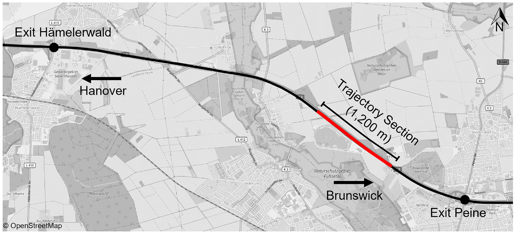
Location of the A2 dataset.
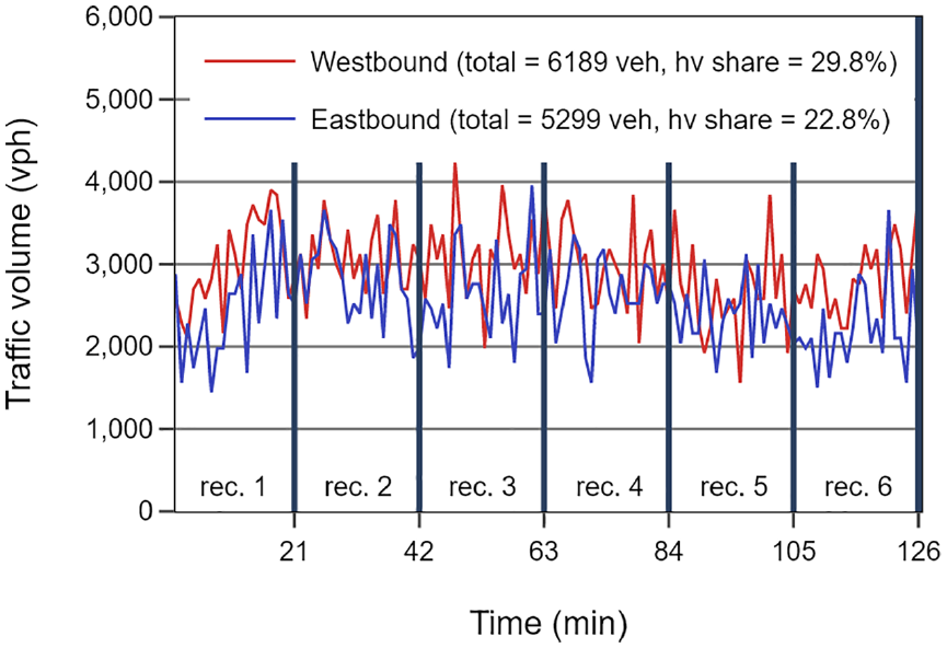
Traffic volume of the A2 dataset.
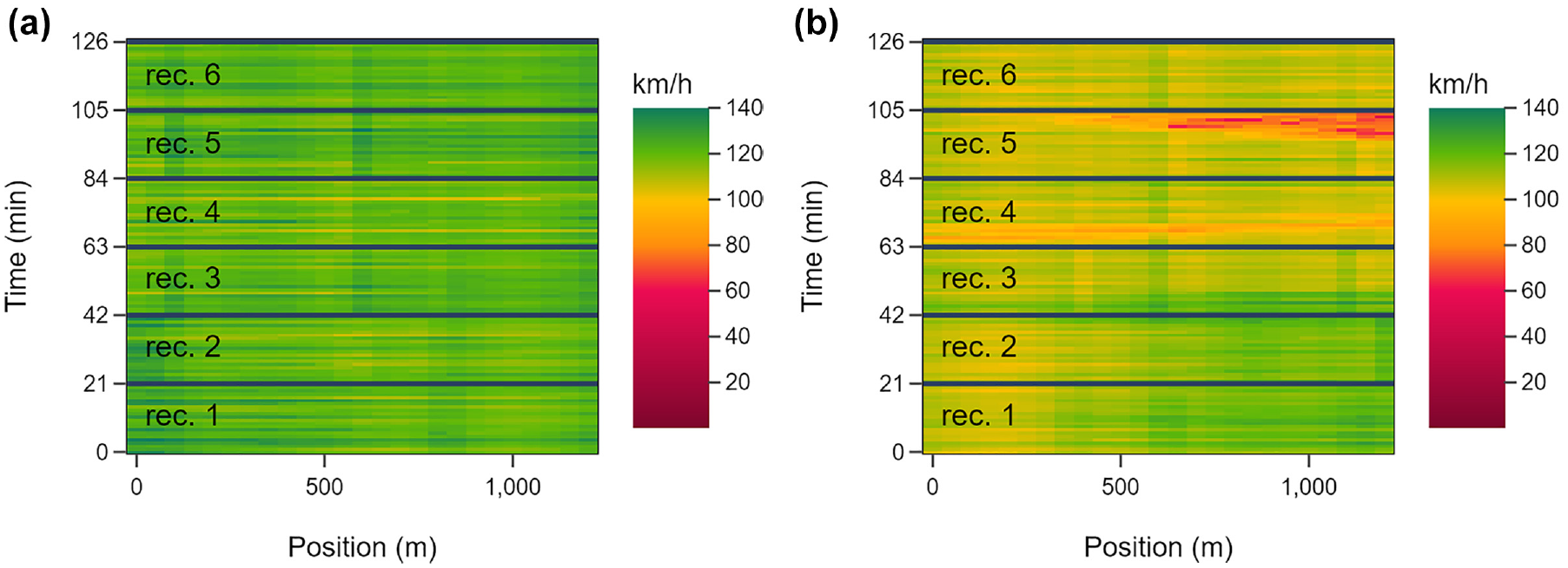
Spatiotemporal evolution of average passenger car speed of the A2 dataset (a) westbound, and (b) eastbound.
The data preprocessing conducted for the A2 dataset is described in the following sections.
Data Preprocessing
Lane Matching
The recorded vehicle trajectories are initially projected onto world coordinates. To be able to determine time headways, we perform a projection onto roadway coordinates and a lane matching. Automatic extraction of map lane boundaries is not used because of the distorted positions of the vehicles. Instead, we carry out the determination of the lane boundaries manually. To support this process, we generate cross-sections at intervals of 10 m, and create histograms of the lateral positions of the intersecting trajectories. The lane boundaries are then placed as close as possible to the minima of the histograms.
Subsequently, the lane boundaries are iteratively improved. For this purpose, we introduce a metric to determine vehicles overtaking each other within the same lane based on the current lane boundaries. The objective is to minimize this metric by slightly adjusting the lane limits.
Vehicle Dynamics Calculation
We compute the speed of a vehicle
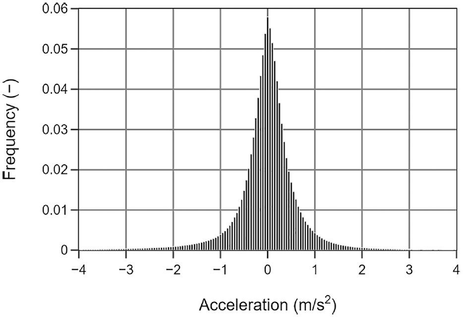
Distribution of acceleration values after data processing.
Headway Calculation
At each time step, we determine the preceding and following vehicles of a vehicle. To achieve this, we cluster the vehicles into groups based on their lane for each time step. Each group is then sorted based on the distance traveled, allowing for retrieval of the preceding vehicles.
Then, we calculate the distances between each vehicle and the surrounding vehicles and, based on these distances, we compute space and time headways. The time headway is based on the speed of the following vehicle.
Application of the Modified Kaplan–Meier Approach
Applying the modified Kaplan–Meier approach requires individual vehicle data from stationary detectors. These data need to be synthesized from the vehicle trajectory datasets and are further referenced as synthetic stationary detectors. To do this, the trajectories are cut every 50 m along the recorded segment (see Figure 5), and for each of these stationary detectors, the current speed of every vehicle and its space headway to the preceding vehicle, as well as the speed difference to the preceding vehicle, are calculated. Based on these values, we determine for each vehicle the probability that it is constrained while driving (see Equation 1). The modified Kaplan–Meier estimation is carried out individually for each of these synthetic stationary detectors, resulting in one desired speed distribution every 50 m along the freeway segment, as well as for the combined data of all synthetic detectors of each direction.
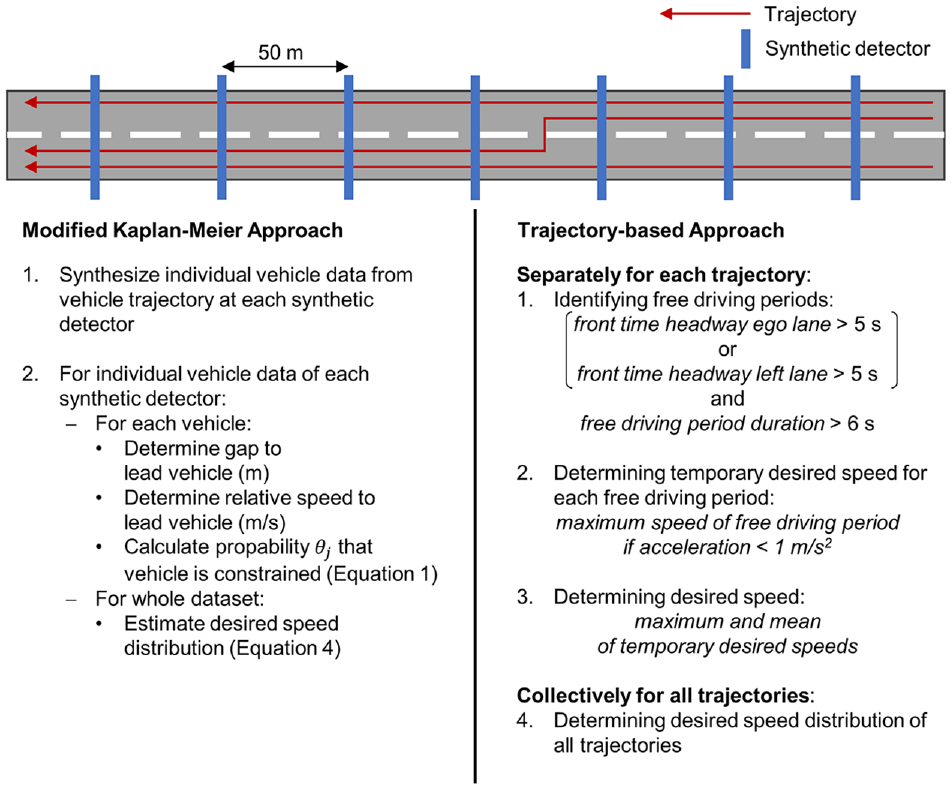
Estimating desired speed distributions with the modified Kaplan–Meier approach and determining desired speeds based on vehicle trajectory data.
Determining Desired Speeds Based on Vehicle Trajectory Data
The modified Kaplan–Meier approach is limited to observing a vehicle only at a single point in space and time. In contrast, the method proposed in this study utilizes vehicle trajectories to determine desired speeds as we examine a vehicle over a specific time duration and distance. In the first step, we identify free driving periods during which an ego vehicle is driving without being constrained by preceding vehicles. We define being constrained as having a front time headway of less than a threshold of 5 s. Other studies use smaller thresholds (e.g., Geistefeldt [ 5 ]), but to ensure that the vehicles are unconstrained we opt for this conservative definition. This assessment considers both the preceding vehicle in the same lane and in the left lanes of the ego vehicle, whereas the headway to at least one of these preceding vehicles must be higher than the threshold. To ensure that the driver is conscious about a free driving period, only periods exceeding a minimum free driving period duration of 6 s are considered further. This represents a duration in which a driver has enough time to perceive their current situation and potentially adjust their speed to match their desired speed. This parameter value is a best guess that we find reasonable but have not empirically investigated so far. For this reason, its impact on the proportion of vehicles for which a desired speed can be determined will be discussed later as part of a sensitivity analysis.
In the next step, we determine a temporary desired speed for each free driving period. For this purpose, we identify the highest speed attained during the period and verify whether the vehicle’s acceleration, by the time it reaches this maximum speed, remains below a threshold of 1
If multiple free driving periods are identified for a vehicle, various temporary desired speeds may result. To determine a desired speed distribution for the collective of vehicles on the segment, these temporary desired speeds need to be aggregated into a single desired speed value for each vehicle. Several approaches can be used for this aggregation, such as selecting the maximum temporary desired speed, the mean of the temporary desired speeds, or the temporary desired speed that occurs most frequently. Since this study is based on trajectory datasets with a length of 1,200 m, and thus only a limited amount of free driving periods are expected to be identified per vehicle, we carry out the estimation with the mean and maximum temporary desired speed and discuss the results. The differences between these temporary desired speeds and the stability of the desired speed over the course of the road segment are examined further.
Results
Modified Kaplan–Meier Approach
We applied the Kaplan–Meier approach separately to the data from each individual synthetic detector, allowing the estimation of desired speed distributions at 50-m intervals for both driving directions. Figure 6 shows the resulting desired speed distributions. The color shades illustrate the different synthetic detectors, with the colors darkening along the driving direction. In the westbound direction, the median of the distributions is approximately 15 km/h higher than in the eastbound direction. This difference could potentially be attributed to the presence of a freeway exit about 1,000 m downstream and the occurrence of merging processes toward the end of the trajectories in the eastbound direction.
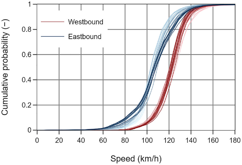
Desired speed distributions of passenger cars for every synthetic detector based on the Kaplan–Meier approach.
Figure 7 depicts the variation of desired speed distributions in 50-m increments along the segment. Each line corresponds to the evolution of a percentile, with the percentiles plotted at 5% intervals. In the westbound direction, the desired speed distributions remain relatively constant, with percentile values as well as the median fluctuating in an interval of 5 km/h, with the median remaining between 120 and 125 km/h. In contrast, in the eastbound direction, it is evident that the dispersion of the desired speed distribution increases with position, particularly as the distance to the exit decreases. Despite this variation, the median of the distribution remains approximately constant at 105 km/h along the trajectory. Interestingly, both the lower and upper percentiles widen equally. This could be because, on the one hand, vehicles may reduce their speed without direct influence from other vehicles, and on the other hand, there tend to be fewer vehicles on the left lane near the exit, providing more space for vehicles staying on the freeway to drive faster.
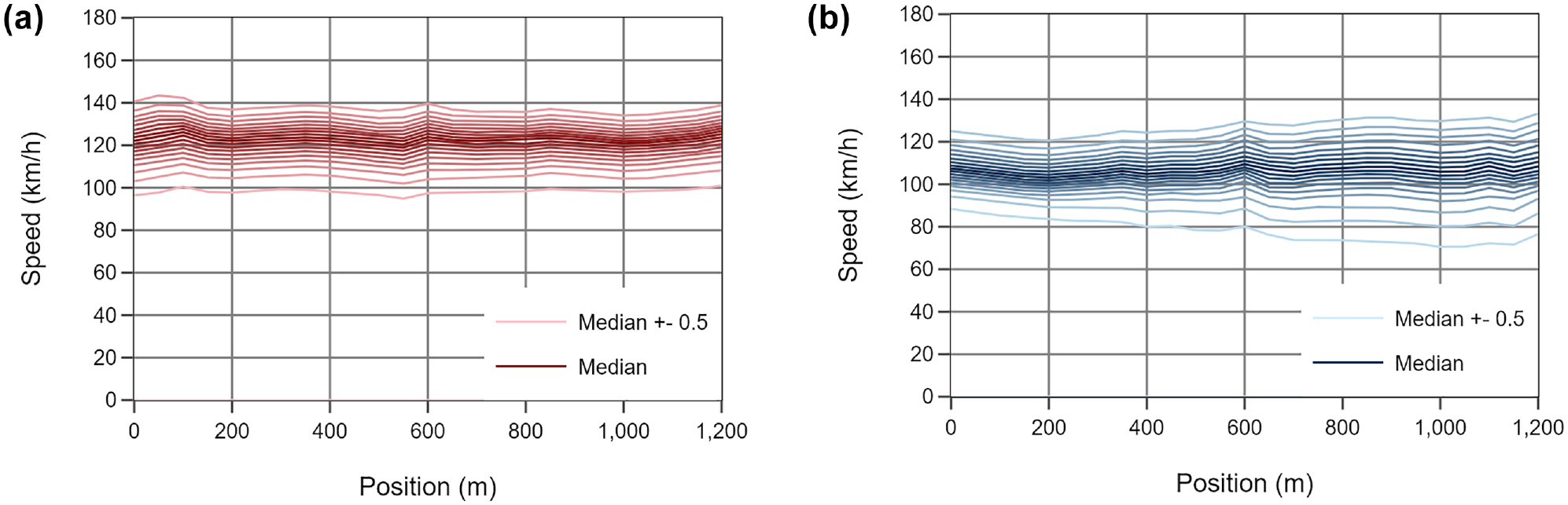
Percentiles of the desired speed distributions of passenger cars estimated with the modified Kaplan–Meier approach (a) westbound and (b) eastbound.
Trajectory-Based Approach
Estimating the desired speed from vehicle trajectories enables the examination of the stability of a vehicle’s desired speed throughout the duration of its trajectory. As Figure 8 illustrates, we could only identify one free driving period for most of the vehicles because of the 1,200 m length of the vehicle trajectory dataset. To examine the intra-vehicle stability of the desired speed, we focused only on vehicles for which more than one free driving period could be identified. To assess the intra-vehicle stability of the desired speed, the difference between a vehicle’s highest and lowest temporary desired speeds is determined. While other statistical metrics like the standard deviation of the temporary desired speeds are conceivable, they have been omitted because of the limited amount of free driving periods available for evaluation. This maximum desired speed delta exceeds 5 to 7 km/h for 40% of the vehicles, depending on the driving direction.
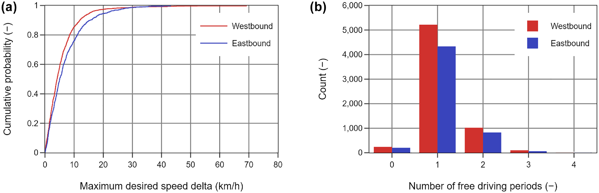
(a) Distribution of maximum desired speed distribution delta for passenger cars with multiple free driving periods, and (b) number of free driving periods per passenger car.
Figure 9 displays the desired speed distributions estimated using the trajectory-based approach. Similar to the results of the modified Kaplan–Meier approach, the westbound desired speed distribution is approximately 15 km/h higher in the median range. As we mentioned above, this difference could potentially be attributed to the presence of a freeway exit about 1,000 m downstream and the occurrence of merging processes toward the end of the trajectories in the eastbound direction. We have considered two variants of the method concerning the determination of the desired speed for each vehicle based on the temporary desired speeds: the maximum and mean of the temporary desired speeds. These results were compared with the estimations obtained with the modified Kaplan–Meier approach, which were computed based on the entire set of synthetic detector data for each driving direction. Because of the limited amount of vehicles for which we have been able to identify multiple free driving periods, the results of the maximum and mean of the temporary desired speed mostly align, as they yield the same result for vehicles with only one free driving period.
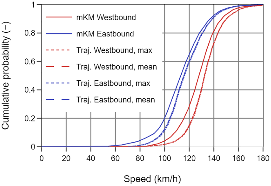
Desired speed distribution of passenger cars estimated with trajectory-based approach (traj.) and modified Kaplan–Meier approach (mKM).
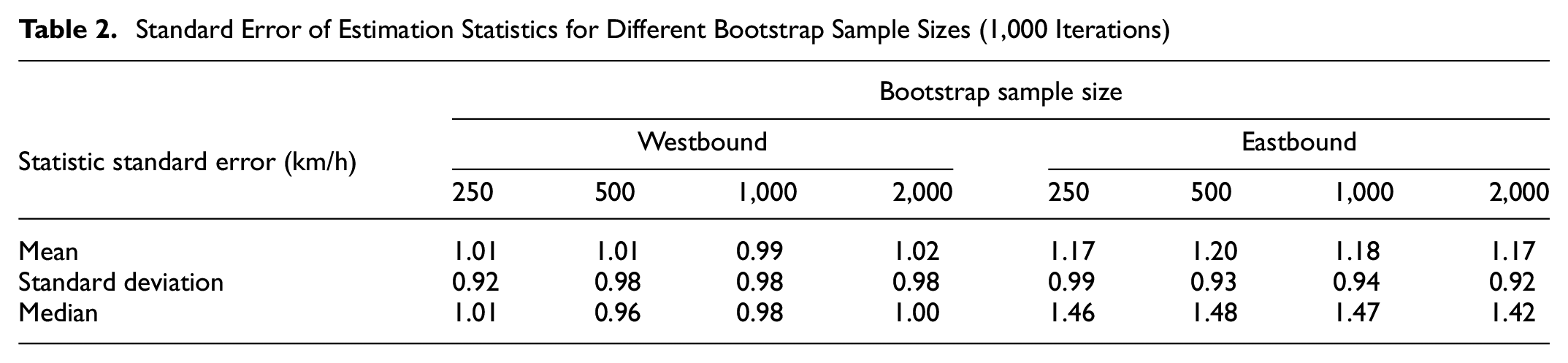
We apply non-parameterized bootstrapping with 1,000 iterations separately for each driving direction to further examine the significance of the obtained results. Table 2 presents the results for the distributions’ mean, standard deviation, and median for different sample sizes. Regardless of the sample size, the median in the westbound driving direction yields a standard error of about 1.0 km/h, and in the eastbound driving direction, it is lower than 1.5 km/h. Comparing the results of the trajectory-based approach with the modified Kaplan–Meier approach, we observed similar outcomes in both driving directions: the shapes of the desired speed distributions largely align, but the values at the median level are approximately 5 to 10 km/h higher with the trajectory-based approach.
Standard Error of Estimation Statistics for Different Bootstrap Sample Sizes (1,000 Iterations)
Discussion
Comparing the proposed trajectory-based approach with the established modified Kaplan–Meier approach indicates that the achieved results are reasonably plausible because they fall within a similar range as those of the modified Kaplan–Meier approach, and the shapes of the desired speed distributions align. The discrepancies can be explained as follows. Since the modified Kaplan–Meier approach relies on stationary detector data, each vehicle is considered only once at a single point in space and time. Therefore, it is possible that a vehicle has not yet reached its desired speed at that particular point and continues to accelerate after passing the stationary detector. Additionally, it is conceivable that apart from the free driving period recorded by the stationary detector, there are other free driving periods for the same vehicle with higher temporary desired speeds. Under these circumstances, it is reasonable that the desired speed distribution obtained through the trajectory-based approach displays higher speeds than the modified Kaplan–Meier approach.
Considering the discrepancies observed both in the application of the modified Kaplan–Meier approach to multiple synthetic detectors and between the results of the modified Kaplan–Meier approach and the proposed trajectory-based approach, it can be concluded that the estimation of desired speed distributions is subject to a certain degree of inaccuracy, ranging between 5 and 10 km/h for the A2 dataset. This should be taken into account when calibrating microscopic traffic flow simulation models.
The question of which method provides the “more accurate” results cannot be easily answered based solely on empirical evidence from the vehicle trajectory dataset. Without knowledge of the actual ground truth, that is, the true desired speed of each vehicle, we lack a definitive benchmark for comparison. Simulation experiments, where a specific desired speed distribution is defined as an input parameter and the presented approaches are used to attempt to reproduce this desired speed distribution from the resulting simulation outcomes, can provide valuable insights.
Nevertheless, this raises the question of whether the concept of a fixed desired speed over time and space accurately reflects reality. As shown in Figure 8, the temporary desired speeds can exhibit considerable variations across different free driving periods (in the A2 dataset, the maximum desired speed delta exceeds 5 to 7 km/h for 40% of the vehicles). Current microscopic traffic flow simulation tools do not consider these intra-vehicle instabilities of desired speed in their models. The extent to which these instabilities influence traffic flow cannot be conclusively determined here and must be addressed in further investigations.
Based on the A2 dataset, Figure 10a illustrates that depending on the position of the synthetic detector and driving direction, approximately 80% of the vehicles are unconstrained according to the modified Kaplan–Meier approach, allowing for direct determination of desired speed. As we do not know the desired speeds of the constrained vehicles, the desired speeds are estimated by applying the product-limit method. In contrast to the modified Kaplan–Meier approach, the trajectory-based approach lacks a mechanism to determine desired speeds for vehicles without a free driving period. This mechanism is not necessarily required here as we were able to identify a free driving period for 96% of the vehicles in both directions (see Figure 10a), allowing for the determination of desired speed.
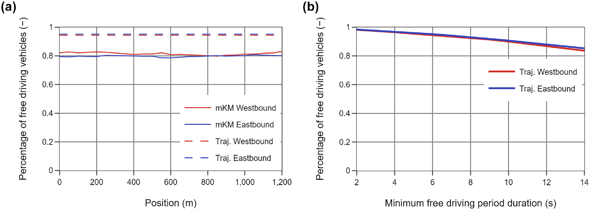
Percentage of free driving passenger cars depending on the used approach (a) and the min. free driving period duration (b).
The percentage of free driving vehicles is influenced by the choice of the minimum free driving period duration parameter. A sensitivity analysis reveals that the percentage of free driving vehicles decreases linearly with increasing the minimum free driving duration (see Figure 10b). We use 6 s as a threshold in this study.
Conclusion and Further Research
Desired speed distributions are crucial input parameters in microscopic traffic flow simulations. However, their determination is not straightforward, especially in situations of high traffic densities, where most vehicles are constrained by surrounding vehicles and cannot attain their desired speeds. The established method for estimating desired speed distributions is the modified Kaplan–Meier approach, which estimates the desired speed distribution based on single vehicle data from stationary detectors using the product-limit method. Nonetheless, the application of this method is limited to a stationary perspective, where each vehicle is only captured at a single point in space and time. In contrast, vehicle trajectory data provides the opportunity to observe each vehicle over a certain distance. In this paper, we propose a novel method for estimating desired speeds from vehicle trajectory data, as no similar approach has been found in the existing literature. This trajectory-based approach is compared with the established modified Kaplan–Meier approach, which is applied to synthesized stationary detector data derived from the vehicle trajectories. Furthermore, we evaluated the intra-vehicle stability of desired speeds using the outcomes obtained from both methods. To conduct our evaluations, we used vehicle trajectories covering a length of 1,200 m on a German freeway. The trajectory dataset covers 2 h of recording time, encompassing both driving directions and a total of 11,488 vehicles.
Applying the modified Kaplan–Meier approach on synthetic detectors at 50-m intervals along the recorded vehicle trajectories revealed that the desired speed distribution widens as the freeway exit is approached, with lower percentiles experiencing a notable decrease in speed. Analyzing the trajectory data demonstrated that 40% of the vehicles exhibited a delta of temporary desired speeds exceeding 5 to 7 km/h between different free driving periods. These findings suggest that the desired speed of a vehicle does not remain constant along its route, although the obtained results are based on only 1,200-m-long trajectories, and longer trajectories are necessary to verify them further.
Comparing our proposed method based on vehicle trajectory data with the established modified Kaplan–Meier approach, it becomes evident that the obtained results are reasonably plausible. The estimated desired speed distributions lie within a comparable range to those of the modified Kaplan–Meier approach, and the shapes of the distributions align. For both approaches, the westbound desired speed distribution is approximately 15 km/h higher in the median range, most probably because of the presence of a freeway exit about 1,000 m downstream and the occurrence of merging processes toward the end of the trajectories in the eastbound direction. The desired speed distributions obtained from the trajectory-based approach are approximately 5 to 10 km/h higher than those estimated by the modified Kaplan–Meier approach. This difference in results is possibly because the trajectory-based approach observes each vehicle over a longer distance rather than just at stationary points. While this finding holds true for both driving directions in the A2 dataset, this investigation should be conducted in the future for additional road segments to validate the findings. Nevertheless, it can be concluded that the estimation of desired speed distributions is subject to a certain degree of inaccuracy. This should be considered in the context of calibrating microscopic traffic flow simulations.
The analysis of the trajectory data enables the identification of a free driving period for almost every vehicle in the A2 dataset, facilitating the determination of desired speeds. However, at higher traffic densities than those present in the current dataset, this approach may not be as straightforward. Future studies should explore and refine the proposed trajectory-based approach to deliver plausible results even when free driving periods cannot be identified for all vehicles. Moreover, all analyses of desired speeds in this study pertain to passenger cars. The extent to which the share of heavy vehicles influences these desired speeds and whether the approach can also be used to estimate desired speeds for heavy vehicles needs to be further investigated in subsequent studies. To extrapolate empirical findings and compensate for the lack of a ground truth, microscopic traffic flow simulations should be employed. Using these simulations, the proposed approach can be applied to various scenarios and traffic densities, allowing for an examination of how well the desired speed distributions defined as input parameters in the simulation can be reproduced by the approach based on the simulation results. Further investigations into the intra-vehicle stability of desired speed also require additional vehicle trajectory datasets, ideally covering longer stretches, such as the I-24 MOTION project ( 27 ), whose data was not available at the time of this study. In this context, it is important to explore the potential impact of intra-vehicle instability of desired speed on traffic flow and to assess whether and how such variability should be represented in microscopic traffic flow simulations.
Footnotes
Author Contributions
The authors confirm contribution to the paper as follows: study conception and design: M.V. Baumann, C.M. Weyland, L. Fuchs, J. Grau, P. Vortisch; data collection: M.V. Baumann, J. Ellmers; analysis and interpretation of results: M.V. Baumann, C.M. Weyland; draft manuscript preparation: M.V. Baumann, C.M. Weyland, J. Ellmers, L. Fuchs. All authors reviewed the results and approved the final version of the manuscript.
Declaration of Conflicting Interests
The authors declared no potential conflicts of interest with respect to the research, authorship, and/or publication of this article.
Funding
The authors disclosed receipt of the following financial support for the research, authorship, and/or publication of this article: This paper is based on research funded by the German Federal Ministry for Digital and Transport, represented by the Federal Highway Research Institute.