Sage Journals: Discover world-class research

Abstract

The long-term monitoring of transportation infrastructure assets at a lower cost and with short mobilization time is of significant interest to both state and federal transportation agencies in the U.S. Because of the significant improvement in spatial and temporal resolution of synthetic aperture radar (SAR) remote sensing systems and a notable reduction in the cost of data acquisition, SAR has now become a viable method to provide economic and rapid condition assessment of transportation assets. A research study was developed and performed to comprehensively perform the inspection and characterization of a pavement surface based on the amplitude of backscattering of an X-band radar. In situ characterization of the test site was first performed using traditional inertial profilers and aerial photogrammetry with unmanned aerial vehicle (UAV) surveys. The results from these in situ methods were compared with the corrected amplitude of the SAR data, which indicated that the distribution of surface roughness values computed from the inertial profiler, UAV, and SAR exhibited similar probability densities at various segmental lengths considered in this study. This suggested that the problematic areas that are evident during in situ characterization can be delineated and quantified based on the normalized radar cross section of the pavement surface. Overall, the outcome of this research exhibits the potential of SAR for future transportation asset management undertakings, and the systematic framework developed as a part of this research could be of significant interest to engineers and transportation practitioners.

Keywords

infrastructure geology and geoenvironmental engineering geotechnical instrumentation and modeling instrumentation development pavements pavement condition evaluation measurement remote sensing synthetic aperture radar (SAR)transportation assets management unmanned aerial vehicle (UAV)profiler

The transportation network in the U.S. has 4.2 million miles of highway with 3,261 billion vehicle miles traveled as of 2019 ( 1 ). The total expenses and revenues accounted up to $235 billion and $146 billion, respectively, in the financial year 2018. However, more than 50% of interstate miles and 70% of major arterial miles have been reported to have an International Roughness Index (IRI) value greater than 60 ( 1 ). With an increase in the serviceability age of transportation infrastructures, a need for strategic planning and management to keep the functioning of the transportation network in an acceptable condition and at a reasonable cost is of paramount importance ( 2 ). “Moving Ahead for Progress in the 21st Century” (MAP-21) law and “Fixing America’s Surface Transportation” (FAST) Act required each state to prepare a risk-based assets management plan for pavement and bridges which are part of the National Highway System (NHS) to assess the conditions and performance of the system. Transportation asset management (TAM) is defined as a strategic and systematic process of operating, maintaining, and improving the condition of transportation assets to a good or acceptable state at minimum cost with a consideration of both engineering and economic aspects in the development of maintenance, preservation, repair, rehabilitation, and replacement actions ( 3 – 7 ). Conditions of pavement and bridges within the NHS are assessed either annually or biennially; however, assets outside NHS, as well as other right-of-way (ROW) assets, do not have any mandatory condition assessment requirement. Such a gap in data has limited the scope of the TAM plan as these assets have significant importance in the lifecycle of a transportation system as a whole system. A long-term consistent monitoring program for assets such as pavements, highway embankments, and earth retaining systems at a reasonable cost and with a quick mobilization can provide the necessary data to expand the current mandated scope of TAM.

Federal requirement (23 CFR Part 490) mandates U.S. state DOTs to report the condition of pavement—as IRI, rutting, faulting, and cracking percentage—of interstates and non-interstate NHS to the Federal Highway Administration (FHWA). In standard practice, IRI is reported based on American Association of State Highway and Transportation Officials (AASHTO) M328-14 and R56-14 using data from inertial profilers which are required to be collected annually or biennially ( 8 – 10 ). Such a large temporal gap between two acquisitions may fail to identify deteriorating pavement sections; however, increasing the frequency of such acquisitions poses logistical and economic challenges. Therefore, remote sensing platforms have established themselves as data sources that can complement traditional measurement techniques at a lower cost and a shorter turnaround time. Remote sensing is a process of collecting and interpreting information about the environment from a distance (typically using sensors and instruments that are located on aircrafts or satellites). Remote sensing can be a useful tool for monitoring transportation and geotechnical assets network by providing valuable information about its condition and spatial location ( 11 – 13 ). Digital photogrammetry using structure-from-motion (SfM) algorithms is a type of remote sensing technique that has been used for creating high-resolution 3D models of the real world using a set of overlapping 2D images which is based on computer vision and visual perception principles ( 14 – 17 ). Use of unmanned aerial vehicles (UAVs) has increased significantly in 3D mapping of civil infrastructure that leverage the SfM algorithm to accurately reconstruct the scene at very high resolution—up to sub-centimeter ( 12 , 16 , 18 , 19 ). SfM algorithms detect key features in each overlapping 2D image and track these 2D feature between the images which are then reconstructed into features with 3D positions.

Although data from UAVs provide very detailed information on the site, issues such as weather constraints, flight permission, and flight duration present significant challenges in its application ( 18 , 20 ). Use of radar remote sensing satellites for monitoring can overcome these challenges faced by UAVs. Orbital synthetic aperture radar (SAR) is a type of remote sensing system that can collect high-resolution, day-and-night, and weather-independent images of the earth’s surface. The radar transmits electromagnetic pulses that interact with the earths’ surface and receives backscattered signals as amplitude and phase. The amplitude of the backscattered signal represents the strength of the radar echo received by the antenna. It is dependent on the physical properties, such as geometry and roughness, and electrical properties, such as the permittivity of the incident surface ( 21 , 22 ). Before implementing these platforms for pavement condition assessment, it is imperative to understand the background on the working mechanism and protocols for data collection and analysis as discussed in the following section.

Background

The inertial profiler system includes instruments designed to measure the surface profile of a pavement while moving at a given highway speed. The profiler utilizes the data from an accelerometer, which provides an inertial reference or instantaneous height using a non-contact laser that measures the distance between the accelerometer and the ground, and a speedometer to gauge the longitudinal distance traveled ( 23 ). The profile elevation is calculated using double integration of accelerometer data and height from the non-contact sensor, as shown in Equation 1. IRI is a numerical approach to compute the roughness/smoothness of a road from this single longitudinal surface profile data which is smoothed with moving average of base length 250 mm and filtered using a quarter-car simulation with golden car parameters at 80 km/h. ( 24 ):

Profile elevation = (\iint A) - H

(1)

where

A = inertial reference accelerometer, and

H = height relative to inertial reference using non-contact continuous measurement.

Advances in digital sensors for taking images and storage technology made it possible to capture numerous high-resolution images in an affordable way in the mid-to-late 2000s. SfM is a photogrammetric method used in UAVs to generate high-resolution 3D structures for a series of overlapping images that are typically derived from moving sensors ( 15 ). Scale-and-rotation-invariant key features are identified in each of these overlapping images which are then used to estimate camera pose and scene geometry to extract point clouds in image-space ( 15 , 25 ). The 3D point clouds are transformed into a real-world co-ordinate system using ground control points (GCPs) during the post-processing step. A redundant network of these evenly distributed GCPs, which are high-contrast targets both in the field and point cloud, is established to account for any potential issues with sparse data or errors in SfM reconstruction ( 17 , 25 ).

SfM is used in cases where the subject is closer to the sensor, such as UAV platforms, thus limiting itself to monitoring from relatively close distances. Orbital remote sensing platforms, such as SAR, have seen a significant boom in the last two decades that has the potential to provide consistent long-term monitoring of civil engineering assets at competitive cost from space ( 26 , 27 ). The radar in the orbital platform transmits electromagnetic pulses that interact with the earth’s surface and receives backscattered signals which are then processed to generate an image with each pixel corresponding to the reflectivity of that point on the ground. Radar cross section (RCS or $σ$ ) is the inferred target area based on the ratio of the received response signal intensity and transmitted signal intensity (Equation 2). For a given wavelength and observation angle, RCS is dependent on the physical properties, such as geometry and roughness, and electrical properties, such as permittivity of the incident surface. Depending on the type or orientation of the area used to normalize RCS several measures are calculated. Radar brightness ( $β^{0}$ ) is the quantity measured by a SAR sensor which is equal to RCS normalized with a solid rectangle defined in the slant range plane representing the ground surface. The normalized radar cross section (NRCS), also known as sigma nought ( $σ^{0}$ ) is calculated by normalizing RCS with the actual geometrical area on the ground surface (Equation 3). $σ^{0}$ is the primary value of interest to the stakeholder as it quantifies the ground surface response and minimizes the radiometric difference caused by changes in incidence angles, acquisition geometry, and look direction ( 22 , 28 ).

σ = \frac{I_{rec}}{I_{inc}} 4 π R^{2}

(2)

σ^{0} = \frac{β^{0}}{\sin θ_{i}}

(3)

where

$σ$ = RCS (m²),

R = distance between the sensor and the object (m),

I_rec = received signal intensity,

I_inc = transmitted signal intensity,

$β^{0}$ = radar brightness,

$σ^{0}$ = NRCS (m²/m²), and

$θ_{i}$ = local incidence angle between the incoming wave and the normal to the local surface.

The radar response of surfaces such as pavement, low-vegetation fields, and vegetation-free soils is dominated by surface scattering, which is the main contributor to the NRCS. Surface scattering is primarily the function of the roughness of the surface, the wavelength of the SAR sensor used, and the incidence angle. Therefore, for a given wavelength and incidence angle of the SAR sensor, the roughness of the surface becomes the principal contributing factor for the radar response of pavement and alike surfaces.

The majority of U.S. and Canadian transportation agencies at the network level collect surface distresses and smoothness/roughness data to monitor pavement condition which is used to prioritize maintenance or rehabilitation efforts and funding ( 29 , 30 ). Pavement inspection procedures to collect in situ pavement condition data are expensive (average of $50/mile and up to $170/mile in 2004 dollars) and surveys are time-consuming ( 29 , 31 ). Surface distress (i.e., rutting, cracking, raveling, faulting, spalling, punch outs, pumping) and smoothness/roughness (vertical deviation of pavement along the longitudinal pavement profile) change the RCS of the pavement’s surface. Therefore, the RCS of the pavement achieved from high-resolution SAR data can be used an alternative measure of pavement infrastructure condition. The findings of this study demonstrate the potential of using SAR for future TAM endeavors and may be of great interest to engineers and transportation practitioners. The next section discusses the research scope and the framework used in this study to show the utility of SAR in TAM.

Research Scope and Framework

This paper summarizes an investigation into the use of state-of-practice data acquisition method—profiler, sub-orbital remote sensing platform or UAVs, and orbital remote sensing platform—high-resolution SAR on the inspection and characterization of a pavement surface. A summary of the research framework is shown in Figure 1. The site for this case study was the Proving Grounds Research Facilities located at the 2,000-acre RELLIS Campus of Texas A&M University System in Bryan, Texas. This facility contains multiple runways, aprons, and transportation-related pavements. This study includes RTA Zone 2 35C Sect 3 as shown in Figure 2. The pavement test section was characterized in situ using inertial profilers, aerial photogrammetry (using UAVs or drone platform), and NRCS from SAR data. The next section discusses in detail the systematic steps followed to collect and process the data from ground truth points, as well as UAV and satellite-based remote sensing.

Figure 1.

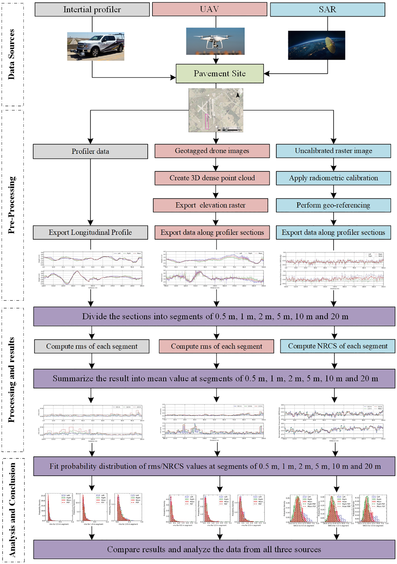
Research flow in this study.

Figure 2.

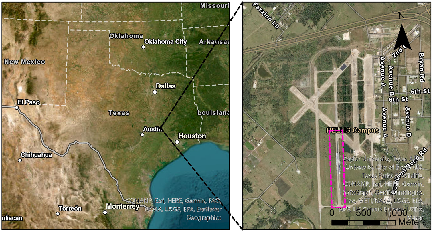
Location of the study site at RELLIS Campus in Texas A&M University.

Data Collection and Pre-Processing

Based on the framework shown in Figure 1, data collection and pre-processing were performed for all three data sources at the site shown in Figure 2. Data from inertial profilers were used to obtain profile information along two sections which are shown in Figure 3a. Similarly, the surface elevation raster that was created by processing data from UAV, and NRCS raster that was created by processing SAR data are shown in Figure 3, b and c , respectively.

Figure 3.

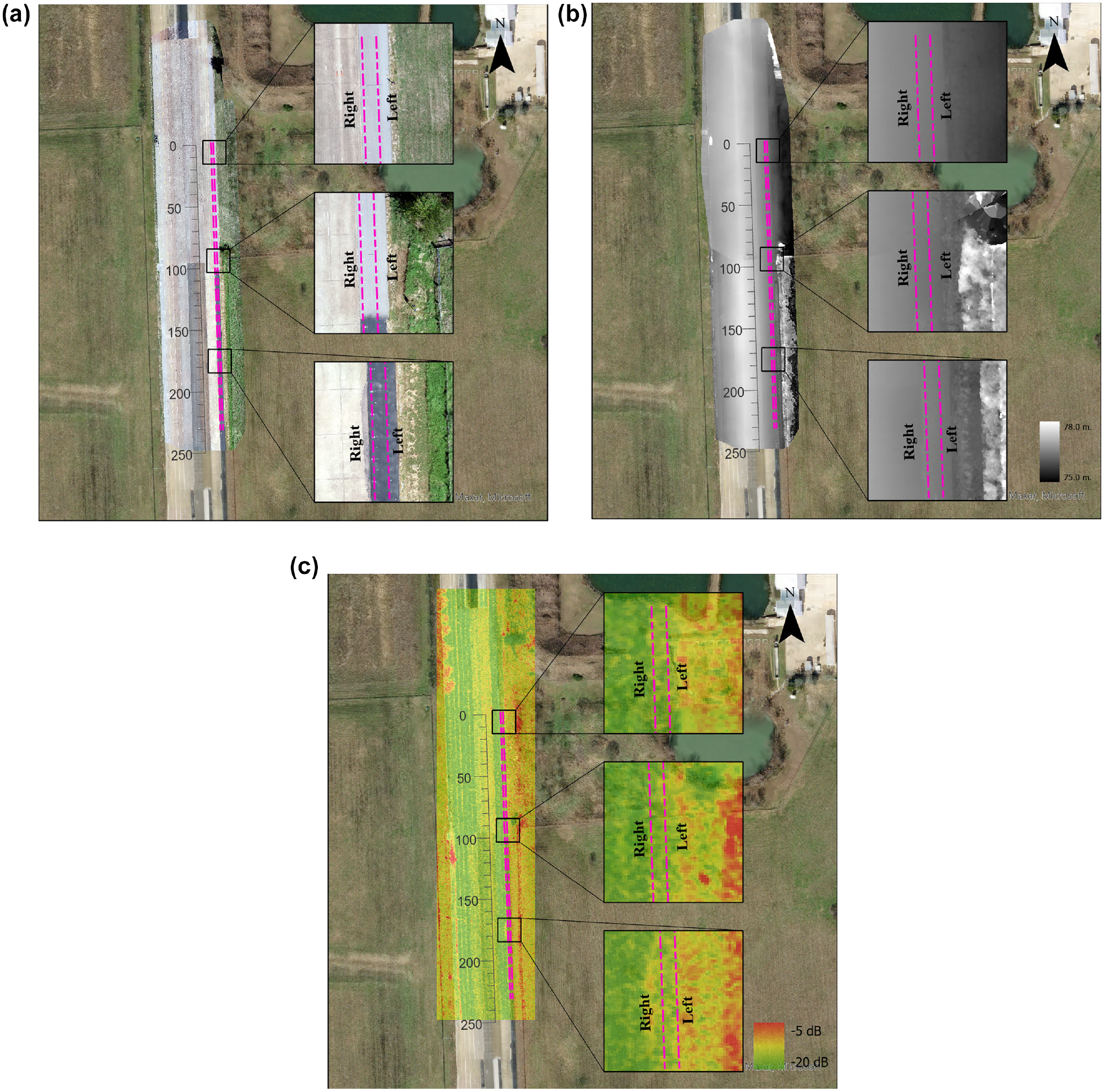
Left and right wheel path for: (a) profiler height data extraction underlain by orthomosaic, (b) digital twin model height data extraction underlain by elevation raster, and (c) normalized radar cross section data extraction underlain by synthetic aperture radar raster.

Inertial Profiler Data

The smoothness/roughness of pavement over a highway network was quantified using data from inertial profilers that measure the relative elevation along the longitudinal profile. The profiler consisted of an instrument sub-system that was mounted on a vehicle with distance measuring, inertial referencing, and non-contact height measurement systems. The instrument system produced and stored profile or elevation data at 3 in. intervals or less by combining data from all sub-systems. Profiler data was obtained from Texas A&M Transportation Institute (TTI)’s Pavement Profiler Evaluation Facility along the section shown in Figure 3a—a dense-graded asphalt test track. The profile data is reported at every 1 in. on dual wheel paths. The data from the profiler was ingested into the FHWA Long-Term Pavement Performance (LTTP) pavement analysis software to generate a simulated profile along the wheel paths. The profile data extracted from this software is shown in Figure 4a.

Figure 4.

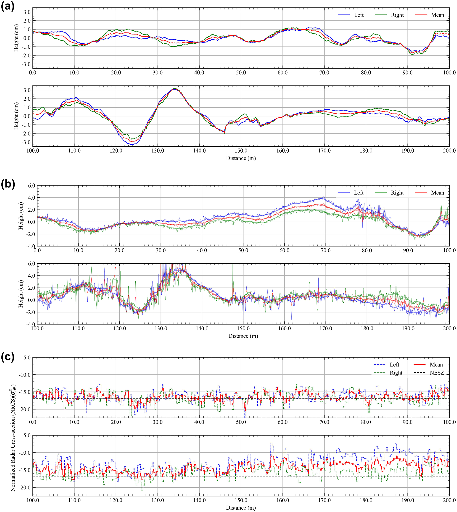
Profile along wheel-paths from: (a) inertial profiler, (b) digital twin model, and (c) synthetic aperture radar data.

UAV data

After obtaining the profiler data, a UAV was used to collect high-resolution aerial images of the site. A reconnaissance survey of the site was used to finalize the flight plan and locations of the GCPs. Data acquisition was performed using the drone platform equipped with an optical sensor, real time kinematics (RTK) navigation system, and post processing kinematics (PPK) geotagging system. The GPS information of each image from the drone platform was corrected using the data from the PPK system after flight. Similar processes have been used by several researchers in correcting the GPS coordinates post-flight ( 18 , 32 , 33 ). The images with corrected GPS information and GCPs were ingested into SfM photogrammetry software to generate dense point cloud, digital surface model (DSM), and ortho-mosaic. DSMs and ortho-mosaics were exported to GIS environments for creating 3D models and extracting elevation data. DSM overlain by the ortho-mosaic facilitated the creation of a digital twin model of the site with a spatial resolution of 0.49 cm. The profile information along the same wheel-paths were extract from the digital twin model, and are shown in Figure 4b.

SAR data

Finally, SAR amplitude data along the same wheel-paths were extracted from the vendor-provided data. Spotlight geocoded terrain corrected (GEO) SAR data product for this site is a one-dimensional raster, where each pixel has been calibrated for radar internal subsystems and corrected for location ( 34 ). The GEO SAR product’s radiometrically calibrated intensities were generated using nine multi-looks of single-look-complex images. The multi-look enhanced the radiometric resolution—the image’s ability to capture reflection differences among pixels without compromising the resolution ( 35 – 37 ). Scale factor provided in the metadata was used to convert the pixel values to RCS using Equation 4 ( 37 ). The raster used in this study was taken by a right-looking Capella-3 satellite with a central frequency of 9.65 GHz (X-band) and a horizontal-horizontal polarization on a descending pass at 33.5° incidence angle ( $θ$ ) and 30.6° look angle. The noise equivalent sigma zero (NESZ) at peak power for this acquisition was −16.979 decibels (dB). These parameters are typical for an X-band high-resolution SAR satellite as shown in several available publications ( 21 , 34 , 38 , 39 ). The GEO product high-resolution SAR imagery from Capella Space was imported into a GIS environment and calibrated using the equation provided in the metadata that resulted in a raster with NRCS in dB scale. SAR data exhibited geo-referring errors when overlain with two reference ortho-mosaics—the first one was from the drone platform and the second one was taken from “Brazos County Imagery” collected as a part of Department of Information Resource Strategic Mapping ( 40 ). Geo-referencing of the SAR data was performed using 1^st-order affine transformation to correctly align the SAR data. The NRCS along the same wheel paths were extracted from the SAR data, and are shown in Figure 4c.

One of the criteria to classify the smoothness/roughness of a surface with respect to the incident electromagnetic wave is the Fraunhofer roughness criterion given by Equation 5 ( 11 , 22 , 41 ). This criterion is useful in modeling the scattering and emission behavior of natural surfaces in the microwave region where the wavelength ( $λ$ ) is of the same order as that of the root mean square (RMS) height of the surface. It is calculated based on the formula shown in Equation 6. In this study, the SAR system is an X-band ( $λ$ = 3.1 cm) radar with incidence angle ( $θ$ ) of 30.6°. Substituting these values in Equation 5 shows that, for s < 0.11 cm, the surface can be considered smooth.

σ_{dB}^{0} = 20 \log_{10} (SC \times D N_{geo})

(4)

where

$σ_{dB}^{0}$ = NRCS (m²/m²) in dB scale,

SC = scale factor provided in the metadata for each scene, and

DN_geo = 16-bit unsigned integer (U Int16) raster value of the image.

s < \frac{λ}{32 \cos (θ)}

(5)

s = [{\frac{1}{N - 1} \sum_{i = 1}^{N} z_{i}^{2} - N {\bar{z}}_{i}^{2}]}^{\frac{1}{2}}

(6)

where

s = RMS height,

$λ$ = wavelength of electromagnetic wave,

$θ$ = incidence angle, and

N = number of samples.

$z_{i}$ = height profile of the surface in consideration.

where,

{\bar{z}}_{i} = \frac{1}{N} \sum_{i = 1}^{N} z_{i}

The RMS heights (roughness) from both the profiler and drone platform, as well as mean NRCS data (radar response) from the SAR satellite, along the two-wheel paths, were processed to compute mean values and probability distribution. This analysis was performed for various segment lengths. Details are discussed in the following sections. The differences in the mean and the probability distributions of each of the methods at various segment lengths can be used as an indicator for the amounts of details perceived and the relationship between the data sources.

Results and Discussion

Characterization Using RMS Heights, NRCS, and Kernel Density Function

The profile height, or the measurement of surface undulations using inertial profiler, were exported from the pavement analysis software for both left and right wheel paths and used for the subsequent roughness analysis. The RMS height of the profile is one of the key metrics that is used to measure surface roughness. Using the RMS, the kernel density estimates were calculated for segments of 0.5 m, 1 m, 2 m, 5 m, 10 m, and 20 m along both wheel paths. The RMS height of the profile was calculated using Equation 6. These intervals were selected as a part of this novel approach to characterize the roughness at different segment lengths. The mean RMS height from the profiler’s data calculated for each segment is shown in Figure 5. The RMS value 0.11 cm threshold, calculated using Equation 5, was delineated using a dotted line (Figure 5). The density histogram of the RMS value and probability density kernel for each segment are shown in Figure 6. The probability density kernel shown is a log-normal kernel which is calculated using maximum likelihood estimation of the RMS data.

Figure 5.

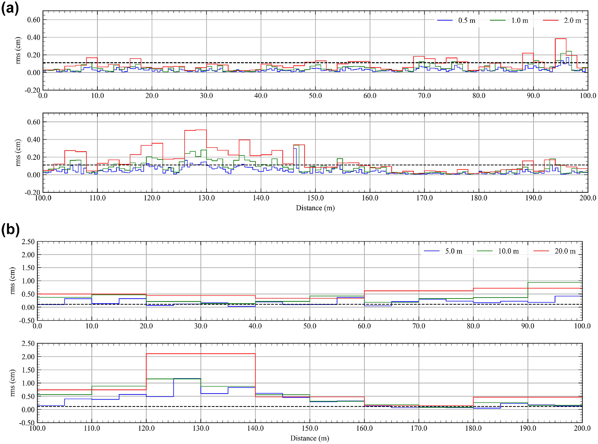
Root mean square (RMS) value of height at segment lengths of: (a) 0.5 m, 1.0 m, and 2.0 m and (b) 5.0 m, 10.0 m, and 20.0 m.

Figure 6.

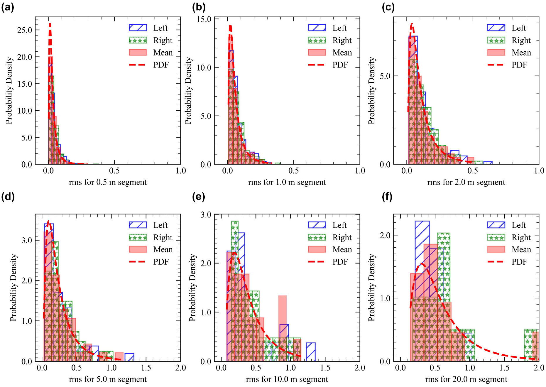
Probability distribution of profiler data root mean square (RMS) for segment lengths of: (a) 0.5 m, (b) 1.0 m, (c) 2.0 m, (d) 5.0 m, (e) 10.0 m, and (f) 20.0 m.

Similar to the inertial profiler, transects along the left and right wheel paths were extracted from the digital twin model. A smoothing moving average filter, with a base length of 250 mm, was applied to the raw data from these transects to smoothen out sharp fluctuation between 1+10 m and 1+40 m (as seen in Figure 4b). In addition to that, the value of height of starting points for each wheel path from the digital twin model is considered the same as the data from the profiler for consistent visualization and comparison of the two results. The smoothed profile was used to compute the surface roughness and kernel density for each of the segments. The RMS height of the smoothed profile is shown in Figure 7. Similar to the inertial profiler, the RMS value 0.11 cm threshold, calculated using Equation 5, is delineated using a dotted line and shown in Figure 7. The density histogram of the RMS value and probability density kernel for each segment is shown in Figure 8. The probability density kernel shown is a log-normal kernel which is calculated using maximum likelihood estimation of the RMS data.

Figure 7.

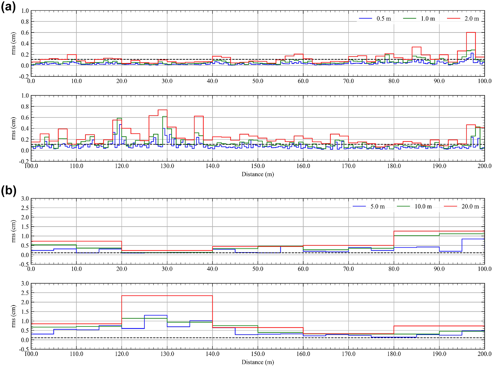
Root mean square (RMS) value of height at segment lengths of: (a) 0.5 m, 1.0 m, and 2.0 m and (b) 5.0 m, 10.0 m, and 20.0 m.

Figure 8.

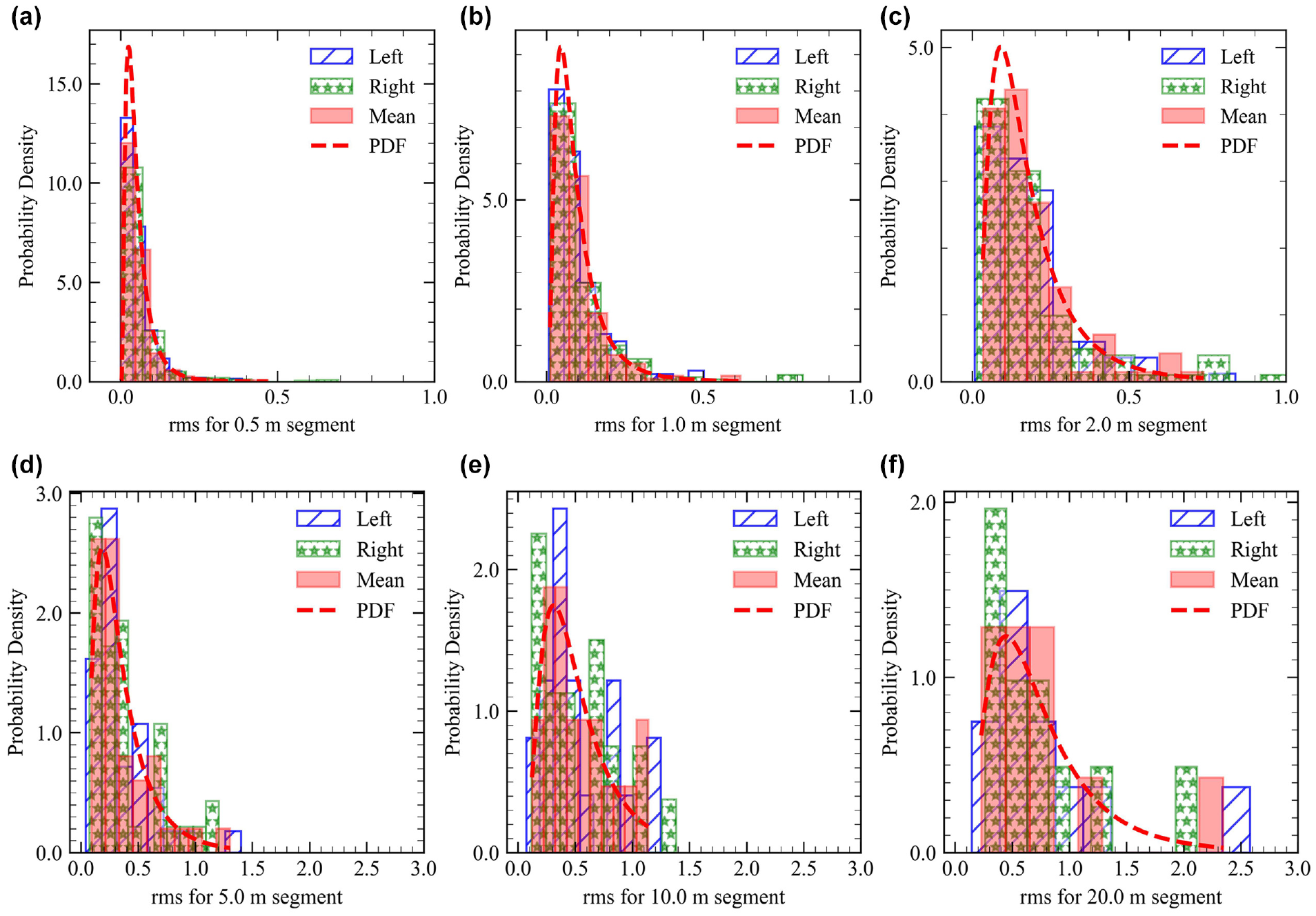
Probability distribution of digital twin model data root mean square (RMS) for segment lengths of: (a) 0.5 m, (b) 1.0 m, (c) 2.0 m, (d) 5.0 m, (e) 10.0 m, and (f) 20.0 m.

Unlike the RMS heights from the inertial profilers’ and digital twin model, the mean value of NRCS along the transects of the two-wheel paths were calculated for segments of 0.5 m, 1 m, 2 m, 5 m, 10 m, and 20 m using the SAR data, as shown in Figure 9. The dotted line in Figure 9 represent the NESZ in dB at peak power. The density histogram of the NRCS and probability density kernel for each segment are shown Figure 10. The probability density kernel shown is a normal kernel which is calculated using maximum likelihood estimation of the NRCS data for each segment.

Figure 9.

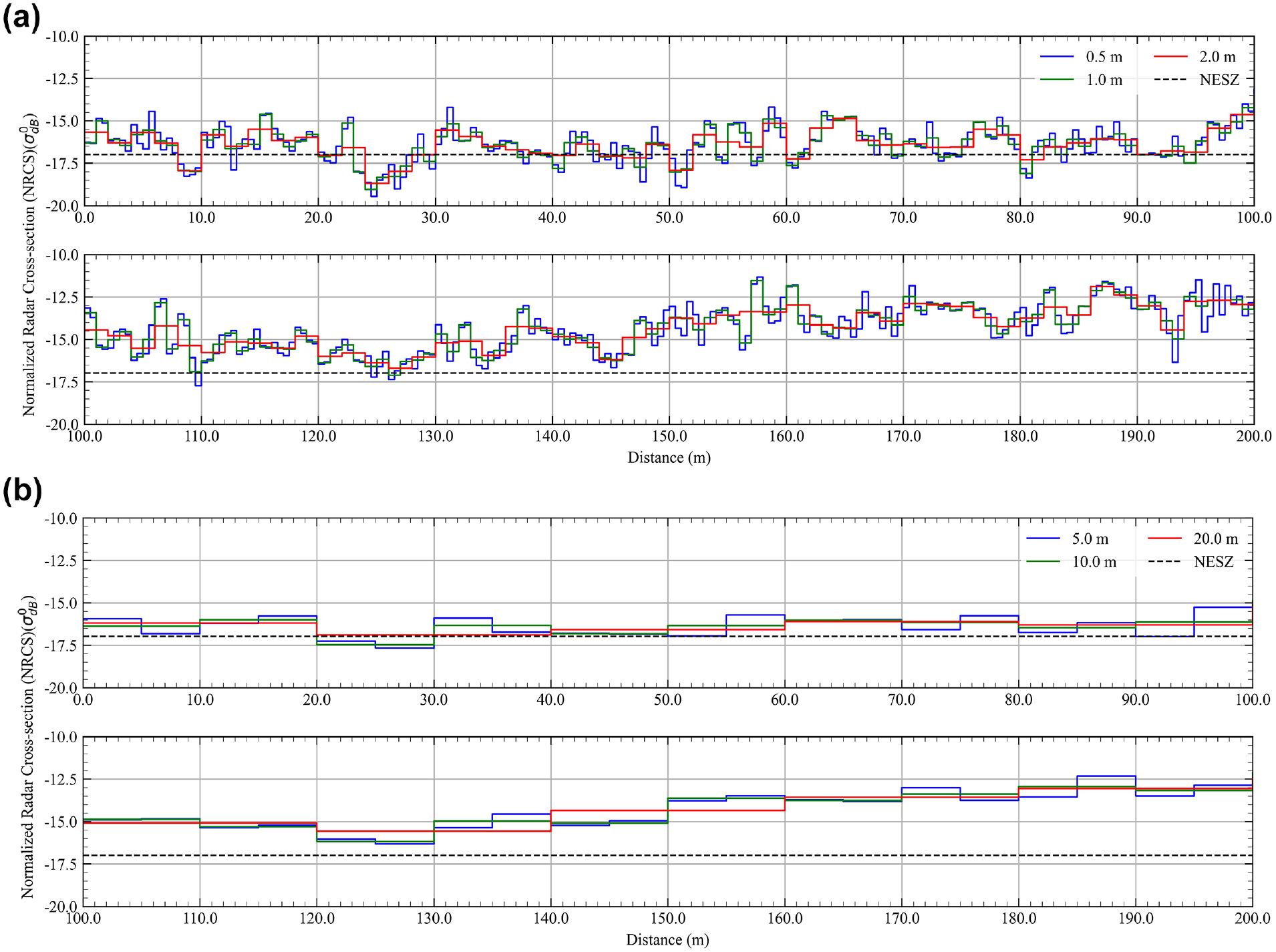
Mean normalized radar cross section (NRCS) at segment lengths of: (a) 0.5 m, 1.0 m, and 2.0 m, and (b) 5.0 m, 10.0 m, and 20.0 m.

Figure 10.

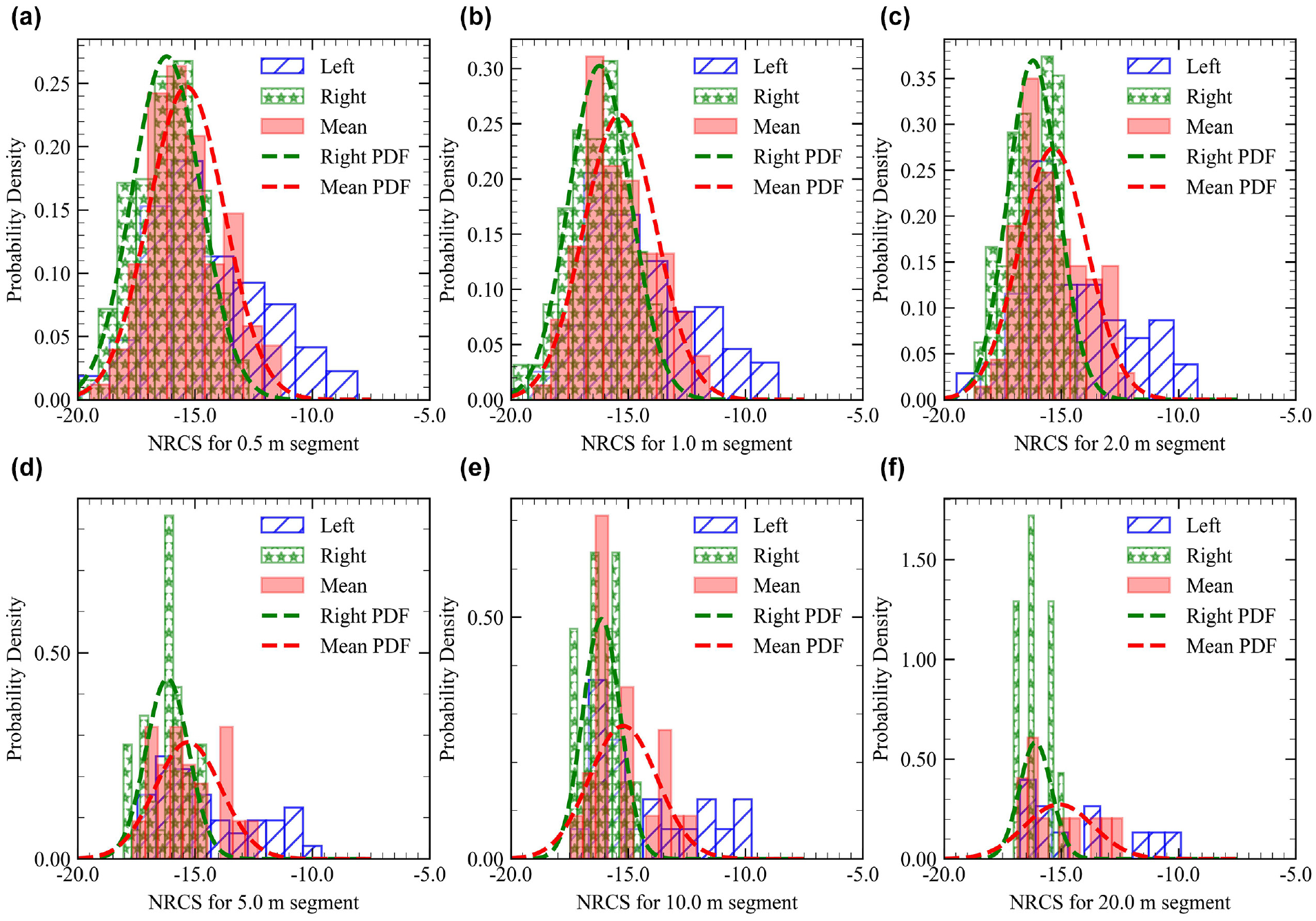
Probability distribution of normalized radar cross section (NRCS) data for segment lengths of: (a) 0.5 m, (b) 1.0 m, (c) 2.0 m, (d) 5.0 m, (e) 10.0 m, and (f) 20.0 m.

Pavement Quality Assessments

As previously discussed and seen Figures 6 and 8, the distribution of the RMS value of the surface from the profiler and digital twin with segment length up to 5.0 m shows a good fit with log-normal kernel Probability Density Function (PDF) but not for 10.0 m and 20.0 m. This suggests that, at longer segment lengths, the low frequency/longer wavelength variation (gradual undulations) in profile becomes significant in the RMS of the surface. The distribution of RMS value for the 5.0 m segments behaves like a cut-off point where the low frequency wavelengths start to become significant. A similar trend in NRCS value from the SAR amplitude data shows a good fit with normal kernel PDF until the 2.0 m segment, as seen in Figure 10. This suggests that both RMS and NRCS values of the transects follow a similar distribution. It is to be noted that NRCS value is in log-scale, therefore the normal kernel PDF was used instead of log-normal. The fit of the normal kernel using right wheel path transect data was better than using mean transect data in the case of NRCS. This can be attributed to the influence of vegetation as well as left-over georeferencing error in spatially geolocating the recorded radar signature. This occurred at the transect near the edge of the pavement, as shown in Figure 3c, and the influence is pronounced after 1+46 ft.

The RMS value of height from the profiler, particularly at a segment length of 5.0 m from 0+00 to 1+00 as shown in Figure 5b, exceeded or was close to the threshold limit for the majority of the stretch (85%) of the total length, as summarized in Table 1. A similar response of NRCS above the NESZ is seen in Figure 9a and b between the same stations for segment length of 2.0 m and 5.0 m, respectively. The RMS value for the segment length of 5.0 m in Figure 5b approaches the threshold value between 0+20 and 0+40. A similar response can be seen in Figure 9, a and b , with the majority of NRCS dropping below or close to NESZ. Significantly higher RMS values for a segment length of 5.0 m dominate the region between 0+90 and 1+50 and the corresponding response in NRCS value can be in Figure 9, a and b .

Table 1.

Percentage of Root Mean Square Value from Profiler and Digital Twin Model above Threshold and Percentage of Mean Synthetic Aperture Radar (SAR) Value above Noise Equivalent Sigma Zero

Segment length/ data source (m)	Profiler		Digital twin model		SAR
Segment length/ data source (m)	0+00 m to 1+00 m	1+00 m to 2+00 m	0+00 m to 1+00 m	1+00 m to 2+00 m	0+00 m to 1+00 m	1+00 m to 2+00 m
0.5	1.5	8.5	2.5	19.5	78.5	98.5
1.0	8.0	30.0	15.0	48.0	84.0	99.0
2.0	32.0	56.0	44.0	92.0	84.0	100.0
5.0	85.0	95.0	95.0	100.0	85.0.	100.0
10.0	100.0	100.0	100.0	100.0	90.0	100.0
20.0	100.0	100.0	100.0	100.0	100.0	100.0

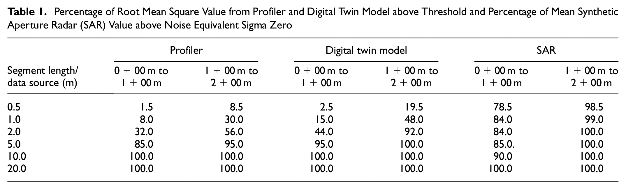
In the case of the RMS value of height from the digital twin model for the 5.0 m segment length, 95.0% of the 0+00 m to 1+00 m section and 100.0% of the 1+00 to 2+00 m section have an RMS value greater than the threshold value, as seen in Figure 7a and summarized in Table 1. This RMS value shows a consistent variation with NRCS value for 0+00 to 1+00 m section for segment length of 2.0 m and 5.0 m, as seen Figure 9, a and b , respectively. The majority of the section with RMS value above or close to threshold shows that the NRCS response above the NESZ. 0+60 to 0+70 m section shows some anomalous behavior. A possible reason could be that the RMS value represents the response along the wheel path (capturing small footprint information), whereas the NRCS response is from the area represented by the pixel (capturing the response of a large footprint). The change in RMS value and the corresponding response seen in NRCS is more prevalent in the data from the digital twin model as it tries to represent the actual physical surface and NRCS is the function of its roughness. This suggests that, for an X-band radar of 0.5 m resolution, the NRCS values for 2.0 m and 5.0 m segments show a relationship with the RMS value of the surface at 5.0 m.

NRCS is sensitive to the surface roughness, that is, the RMS value of the surface, and it is evident from this study that the segment length in consideration plays an important role in computing the value of surface roughness in pavements. For instance, segment length of 2.0 m showed consistency in value and probability distribution among all the data sources. Once such scale of sensitivity is established between the NRCS value and segment length, corresponding surface roughness can be computed from the NRCS value. The surface roughness then can be related to established state-of-practice metrics for summarizing the condition of pavement.

Timely and economic assessment of the condition of pavement assets has always been a priority of state and federal agencies to maintain them in acceptable conditions with minimal maintenance cost. Use of orbital remote sensing platforms, such as high-resolution SAR data, are currently available to infer the condition of assets without any field mobilization—which opens a path toward expanding the current mandatory scope of TAM assets. In addition, the short turnaround time from tasking a satellite to generating results makes it possible to rapidly assess the condition of pavements during extreme events. The remotely sensed data can be directly ingested into an existing GIS platform for assets condition computation and visualization. In the case of pavements, ability to summarize the condition of the whole pavement area (2D), rather than just wheel paths (1D) will indeed aid in providing a better picture of the overall pavement condition.

Summary and Conclusions

This study utilized data from multiple sources to compute the pavement characteristics at various spatial scales (i.e., segment lengths) to compare the results of industry standard methods and state-of-art methods and study their potential relationship with satellite remote sensing data. The study presented a novel approach to comprehending the relationship between SAR backscatter data, road surface quality derived from an inertial profiler, and a digital twin model. The results indicated that both the inertial profiler and digital twin model could successfully capture and represent surface roughness characteristics, with their results varying based on the segment length under consideration. With regard to segment length, RMS values from the inertial profiler were lower than those from the digital twin model. This is potentially because of inertial profilers not providing a true representation of the surface. Conversely, the digital twin model generated using SfM photogrammetry data provided a more precise depiction of surface roughness, capturing smaller wavelength variations more accurately.

It was observed that both data sources showcased similar roughness distribution characteristics at certain segment lengths—0.5 m, 1.0 m, 2.0 m, and 5.0 m. At longer segment lengths, both the profiler and digital twin model effectively captured low frequency or longer wavelength variations in profile, demonstrating that the data source and segment length are critical factors when comparing results with SAR data. The analysis also revealed that the NRCS value of the transects, for segments up to 2.0 m, and the RMS value of the surface from both the profiler and digital twin, for segments up to 5.0 m, follow similar distributions. It was observed that the increase in RMS value did not result in a corresponding increase in the NRCS value, suggesting a potential non-linear relationship. Additionally, it was found that, for X-band radar with 0.5 m resolution, the NRCS value for a 2.0 m segment showed a potential relationship with the RMS value of the surface. This could provide a pathway for the development of refined models to understand the interaction between radar backscatter signals and the condition of road surfaces.

Overall, this research contributes valuable insights to understanding how different remote sensing methodologies can be leveraged to assess road surface conditions. The cost of each SAR scan typically starts at $500 (for 4 × 4 km footprint at 1 m spatial resolution) from commercial vendors. The scanned area not only consists of the data on the pavements but also other assets within the ROW which will help asset managers infer information about the condition of pavement and other ROW assets. However, the cost of processing and handling these SAR data in regard to pavement inspection and management has not been established in this study and should be considered in the future scope. Further studies should aim to perform such analysis on a wide range of sections with varying pavement conditions, refine these methodologies, and develop models that can predict the relationship between SAR backscatter data and road surface quality, offering enhanced tools for monitoring infrastructure and incorporating it as a data source for TAM.

Footnotes

Acknowledgements

The authors acknowledge the support of:

• Texas A&M Transportation Institute (TTI)—Dr Emmanuel Fernando and Dr Charles Gurganus

• Capella Space Inc.—Mr Jason Brown and Mr Chad Baker

• L3 Harris Geospatial—Mr Andrew Fore

• Texas A&M AgriLife—Dr Javier M. Osorio Leyton

• Texas A&M University—John Rios, Jr and Ayush Kumar

• Texas A&M RELLIS Campus—Brad Hall

• Michigan State University—Dr Surya Congress

• PPK platform—Loki PPK system

• Photogrammetry software—Pix4D Mapper

• GIS Environments—ArcGIS Pro and ENVI

• SAR vendor—Capella Space

• Data processing and plotting—Python/Matplotlib

• FHWA/LTTP software—ProVAL

• GIS data—Planet labs, Texas Geographic Information Office (TxGIO), OpenTopography

Author Contributions

The authors confirm contribution to the paper as follows: study conception and design: A. Gajurel, A. Puppala, N. Biswas; data collection: A. Gajurel, N. Biswas, H. Chimauriya; analysis and interpretation of results: A. Gajurel, A. Puppala, N. Biswas, H. Chimauriya; draft manuscript preparation: A. Gajurel, A. Puppala, N. Biswas, H. Chimauriya. All authors reviewed the results and approved the final version of the manuscript.

Declaration of Conflicting Interests

The author(s) declared no potential conflicts of interest with respect to the research, authorship, and/or publication of this article.

Funding

The author(s) disclosed receipt of the following financial support for the research, authorship, and/or publication of this article: U.S. DOT’s Transportation Consortium of South-Central States (Tran-SET) Region 6’s University Transportation Center (Award #22PTAMU04); and National Science Foundation (NSF) Industry-University Cooperative Research Center (I/UCRC) program funded Center for Integration of Composites into Infrastructure (CICI) site at Texas A&M University, College Station, Award # 1464489 (Phase I) and Award # 2017796 (Phase III).

ORCID iDs

Amit Gajurel

Anand J. Puppala

Nripojyoti Biswas

Hiramani Raj Chimauriya

References

USDOT. National Transportation Statistics 2021. U.S. Department of Transportation, Bureau of Transportation Statistics, Washington, D.C., 2021.

ASCE. A Comprehensive Assessment of America’s Infrastructure. 2021. Infrastructure Report Card for America’s Infrastructure. https://infrastructurereportcard.org/wp-content/uploads/2020/12/National_IRC_2021-report.pdf. Accessed July 12, 2023.

AASHTO. AASHTO Transportation Asset Management Guide: A Focus on Implementation, 2nd ed. American Association of State Highway and Transportation Officials, Washington, D.C., 2020.

Anderson

S. A.

Schaefer

V. R.

Nichols

S. C.

Taxonomy for Geotechnical Assets, Elements, and Features. In TRB 95th Annual Meeting Compendium of Papers, Transportation Research Board of the National Academies, Washington, D.C., 2016.

Mazzanti

Toward Transportation Asset Management: What Is the Role of Geotechnical Monitoring?

Journal of Civil Structural Health Monitoring, Vol. 7, No. 5, 2017, pp. 645–656.

Vessely

Robert

Richrath

Schaefer

V. R.

Smadi

Loehr

Boeckmann

Geotechnical Asset Management for Transportation Agencies, Volume 1: Research Overview. Report No. 903. National Academies of Science Engineering and Medicine, Washington, D.C., 2019.

Vessely

Robert

Richrath

Schaefer

V. R.

Smadi

Loehr

Boeckmann

Geotechnical Asset Management for Transportation Agencies, Volume 2: Implementation Manual. The National Academies Press, Washington, D.C., 2019.

National Performance Management Measures. Fed. Reg. Sect. 23 CFR 490 Jan 3, 2017 p. 1399. https://www.ecfr.gov/current/title-23.

Grogg

Van

Rozycki

Vaughn

Roff

Clarke

Beatty

Buck

Christenson

Chang

FHWA Computation Procedure for the Pavement Condition Measures. Report No. FHWA-HIF-18-022. Federal Highway Administration, Washington, D.C., April 2018, p. 84.

10.

Pierce

L. M.

McGovern

Zimmerman

K. A.

Practical Guide for Quality Management of Pavement Condition Data Collection. Report No. DTFH61-07-D-00028. US Department of Transportation, Washington, D.C., February 2013.

11.

Jensen

J. R.

Remote Sensing of the Environment: An Earth Resource Perspective. Pearson, Essex, UK, 2014, 614 p.

12.

Stark

T. D.

Oommen

Ning

Remote Sensing for Monitoring Embankments, Dams, and Slopes. American Society of Civil Engineers, Reston, VA, 2021.

13.

Planet Labs PBC. Planet Application Program Interface: In Space for Life on Earth. Planet, 2023. https://api.planet.com.

14.

Marr

Nishihara

H. K.

Representation and Recognition of the Spatial Organization of Three-Dimensional Shapes. Proceedings of the Royal Society of London. Series B. Biological Sciences, Vol. 200, No. 1140, 1978, pp. 269–294.

15.

Snavely

Seitz

S. M.

Szeliski

Modeling the World from Internet Photo Collections. International Journal of Computer Vision, Vol. 80, No. 2, 2008, pp. 189–210.

16.

Rathje

E. M.

Franke

Remote Sensing for Geotechnical Earthquake Reconnaissance. Soil Dynamics and Earthquake Engineering, Vol. 91, 2016, pp. 304–316.

17.

Congress

S. S. C.

Puppala

A. J.

Lundberg

C. L.

Total System Error Analysis of UAV-CRP Technology for Monitoring Transportation Infrastructure Assets. Engineering Geology, Vol. 247, 2018, pp. 104–116.

18.

Congress

Puppala

Eye in the Sky: Condition Monitoring of Transportation Infrastructure Using Drones. Proceedings of the Institution of Civil Engineers: Civil Engineering, Vol. 176, No. 1, 2022, pp. 40–48.

19.

Turner

Lucieer

De Jong

Time Series Analysis of Landslide Dynamics Using an Unmanned Aerial Vehicle (UAV). Remote Sensing, Vol. 7, No. 2, 2015, pp. 1736–1757.

20.

Shakhatreh

Sawalmeh

A. H.

Al-Fuqaha

Dou

Almaita

Khalil

Othman

N. S.

Khreishah

Guizani

Unmanned Aerial Vehicles (UAVs): A Survey on Civil Applications and Key Research Challenges. IEEE Access, Vol. 7, 2019, pp. 48572–48634.

21.

Flores

Herndon

K. E.

Thapa

R. B.

Cherrington

, eds. The Synthetic Aperture Radar (SAR) Handbook: Comprehensive Methodologies for Forest Monitoring and Biomass Estimation, 1st ed. SERVIR Global Science Coordination Office, Huntsville, AL, 2019. https://gis1.servirglobal.net/TrainingMaterials/SAR/SARHB_FullRes.pdf. Accessed March 18, 2023.

22.

Woodhouse

I. H.

Introduction to Microwave Remote Sensing. CRC Press, Boca Raton, FL, 2006.

23.

Sayers

M. W.

The Little Book of Profiling: Basic Information About Measuring and Interpreting Road Profiles. University of Michigan Transportation Research Institute, Ann Arbor, 1998.

24.

Sayers

M. W.

On the Calculation of International Roughness Index from Longitudinal Road Profile. Transportation Research Record: Journal of the Transportation Research Board, 1995. 1501: 1–12.

25.

Westoby

M. J.

Brasington

Glasser

N. F.

Hambrey

M. J.

Reynolds

J. M.

‘Structure-from-Motion’ Photogrammetry: A Low-Cost, Effective Tool for Geoscience Applications. Geomorphology, Vol. 179, 2012, pp. 300–314.

26.

Faghri

Ozden

Yue

Economic Feasibility Study for Pavement Monitoring Using Synthetic Aperture Radar-Based Satellite Remote Sensing Cost-Benefit Analysis. Transportation Research Record: Journal of the Transportation Research Board, 2017. 2645: 1–11.

27.

Moruza

Economic Analysis of InSAR Technology Application in Transportation. In TRB 96th Annual Meeting Compendium of Papers, Transportation Research Board, Washington, D.C., 2017, p. 14.

28.

Small

Flattening Gamma: Radiometric Terrain Correction for SAR Imagery. IEEE Transactions on Geoscience and Remote Sensing, Vol. 49, No. 8, 2011, pp. 3081–3093.

29.

National Academies of Science, Engineering, and Medicine. Quality Management of Pavement Condition Data Collection. The National Academies Press, Washington, D.C., 2009. http://nap.nationalacademies.org/14325.

30.

TxDOT. Pavement Manual. Texas Department of Transportation, Austin, 2021.

31.

Ragnoli

De Blasiis

M. R.

Di Benedetto

Pavement Distress Detection Methods: A Review. Infrastructures, Vol. 3, No. 4, 2018, p. 58.

32.

Thomas

Stallings

Wilkinson

Unmanned Aerial Vehicles Can Accurately, Reliably, and Economically Compete with Terrestrial Mapping Methods. Journal of Unmanned Vehicle Systems, Vol. 8, No. 1, 2020, pp. 57–74.

33.

Zhang

Aldana-Jague

Clapuyt

Wilken

Vanacker

Van Oost

Evaluating the Potential of Post-Processing Kinematic (PPK) Georeferencing for UAV-Based Structure-From-Motion (SfM) Photogrammetry and Surface Change Detection. Earth Surface Dynamics, Vol. 7, No. 3, 2019, pp. 807–827.

34.

Capella Space. Capella Space Synthetic Aperture Radar (SAR) Open Dataset. 2022. https://registry.opendata.aws/capella_opendata. Accessed November 22, 2022.

35.

Lee

J. S.

Speckle Suppression and Analysis for Synthetic Aperture Radar Images. Optical Engineering, Vol. 25, No. 5, 1986, p. 255636.

36.

F. K.

Croft

Held

D. N.

Comparison of Several Techniques to Obtain Multiple-Look SAR Imagery. IEEE Transactions on Geoscience and Remote Sensing, Vol. GE-21, No. 3, 1983, pp. 370–375.

37.

Capella Space. Capella Space SAR Products Specification. Capella Space, San Francisco, 2022, p. 19. https://www.capellaspace.com.

38.

ICEYE. Satellite Data - How to Use Satellite Data for Better Decision Making. 2023. https://www.iceye.com/satellite-data. Accessed April 30, 2023.

39.

Paek

S. W.

Balasubramanian

Kim

De Weck

Small-Satellite Synthetic Aperture Radar for Continuous Global Biospheric Monitoring: A Review. Remote Sensing, Vol. 12, No. 16, 2020, p. 2546.

40.

StratMap. Brazos County Imagery. 2017. https://data.tnris.org/collection?c=1d69eeb7-d3ab-48d9-8899-2d54476832ba&geo=-96.49118042566539,30.621516152695094,-96.47512871786084,30.643167027433336#9.12/30.6569/-96.375. Accessed January 23, 2023.

41.

Ulaby

F. T.

Long

D. G.

Microwave Radar and Radiometric Remote Sensing, 1st ed. The University of Michigan Press, Ann Arbor, 2014.

Application of Satellite-Based Remote Sensing for the Management of Pavement Infrastructure Assets

Abstract

Keywords

Background

Research Scope and Framework

Data Collection and Pre-Processing

Inertial Profiler Data

UAV data

SAR data

Results and Discussion

Characterization Using RMS Heights, NRCS, and Kernel Density Function

Pavement Quality Assessments

Summary and Conclusions

Footnotes

Acknowledgements

Author Contributions

Declaration of Conflicting Interests

Funding

ORCID iDs

References