Sage Journals: Discover world-class research

Abstract

Corrugated metal pipes (CMPs) corrode over time. To maintain structural performance, deteriorated CMPS must be replaced or rehabilitated. Spray-applied pipe liners (SAPLs) are one of the quickest ways to rehabilitate deteriorated CMPs among other ways. Only a few lab tests and finite element studies from the past have been done on this new method. The calibration of a three-dimensional (3D) full-scale finite element method model using test results obtained at the Center for Underground Infrastructure Research and Education laboratory at the University of Texas at Arlington is covered in this paper. The tests were carried out on circular invert cut CMPs that had been rehabilitated with polymeric SAPLs. To repair the invert-cut CMPs, three different thicknesses were used: 0.25, 0.5, and 1-in. The removal of an 18-in. invert from the intact CMP represented the deterioration of the CMP. A full 3D corrugated model was developed to represent the test setup in the FE model using ABAQUS. To perform the calibration process, the load–displacement curves, earth pressure distribution, and strain around the liner were compared to the test results. The comparison of these parameters showed the capability of the model for verification. The verified FE model was used to generate the load–displacement graphs for other thicknesses and elastic modulus of the liner. In addition, the role of the embedment depth is also considered in the analyses in which the maximum deformation of the rehabilitated pipe has decreased by 58.9% with increasing the burial depth of the pipe from 0.4D (D = external pipe diameter) to 1.0D.

Keywords

culverts pile-soil interaction corrugated metal pipe finite element modeling pipe rehabilitation spray applied pipe liners

Corrugated metal pipes (CMPs) are widely used culvert structures in the American highway system. Compared to other types of culverts, CMPs have shorter service life and, with many of them in service, are nearing or are past their service life. Deteriorated CMPs need to be rehabilitated or replaced for the safety and service of the highways. Since both repairing and replacing these culverts can be expensive, rehabilitation has received more attention in recent years because it is generally thought to be a more practical and less disruptive solution. Different rehabilitation methods have been proposed by different departments of transportation (DOTs), material suppliers, and researchers, from open-cut methods to trenchless technology. Trenchless technology holds advantages over the open-cut method as the open-cut method involves disruption and detouring of traffic ( 1 , 2 ). Common trenchless methods include slip lining, cured in place pipe (CIPP), invert paving, and spray-applied pipe lines (SAPLs).

Although SAPL has been in practice for many years, there are limited studies on the structural capacity of these liners along with studies on the structural contribution of host CMPs. One such study was conducted by Garcia and Moore ( 3 ) with a focus on the increase in the strength of the deteriorated buried culverts rehabilitated with the spray-applied cementitious liner. The deterioration of the tested CMPs was mostly located at the invert and haunch. Another detailed study of rehabilitated pipes was made by Masada ( 4 ), which was sponsored by the Ohio Department of Transportation (ODOT). Tests were performed to find the increase in the structural capacity of the deteriorated pipe after the deteriorated pipe’s invert was paved with reinforced concrete according to the ODOT CMS item 611.11 standard field paving procedures. A pool fund project from several DOTs was conducted at the Center for Underground Infrastructure Research and Education (CUIRE) at the University of Texas at Arlington (UTA), with the objectives to comprehensively test and understand the structural capacity of deteriorated CMPs repaired with SAPLs and cementitious liners. In this project, the deterioration of CMPs was represented by the removal of an 18-in. wide piece of invert from an intact CMP ( 5 – 8 ). Control tests were first performed on one intact CMP and one invert-removed CMP to determine the loss in capacity after the invert removal. After the control test, another set of tests were conducted on invert removed CMPs rehabilitated with a SAPL with three different thicknesses: 0.25-in., 0.5-in., and 1-in. Finite element method (FEM) analysis is a useful tool to complement laboratory tests. It has been widely used to simulate buried culverts and evaluate the influence parameters such as cover depth, boundary effects, corrosion, loading pattern, and pipe–soil interaction. El-Sawy ( 9 ) used three-dimensional (3D) FE models to study the effect of different load conditions and soil type. Taher and Moore ( 10 ) used FEM to study the effect of the wall and backfill soil deterioration on the stability of the corrugated culvert. Elshimi ( 11 ) used 3D-FEM to study 86 different long-span box-arch culverts examining the effects of live loads, number of lanes, design truck position, and so forth. Mai et al. ( 12 ) used two-dimensional (2D) FE analysis to study the effect of corrugated wall deterioration whereas Campbell ( 5 ) used 3D FE model to study the effect of corrosion on the structural capacity of corrugated metal culverts. Smith et al. ( 13 ) inspected the effect of grout strength and the presence of a liner on the performance and load-carrying capacity of rehabilitated corrugated steel pipes. Their result indicates that the specimens with high-strength grout presented substantial surges in load-carrying capacity (ten times greater). Garcia and Moore ( 3 ) employed a cementitious spray on liner rehabilitated pipelines under the single axle configuration at 1,200 mm of cover. After rehabilitation, the pipelines exhibited higher circumferential bending stiffness and their behavior is more like rigid pipes. Ezzeldin and El Naggar ( 14 ) operated FE modeling to study the behavior of buried culverts under different parameters such as cover depth, boundary effects, loading pattern, and pipe–soil interaction. Their results indicate that the design of buried corrugated steel structures has a direct relation to the modeling approach.

The review of the aforementioned and additional literature showed a lack of a well-verified full-scale 3D FE model of deteriorated and rehabilitated CMPs. In addition, many previous studies, such as those of Ezzeldin and El Naggar ( 14 ) and Kunecki and Kubica ( 15 ), used an equivalent smoothed surface approach to model corrugated pipes without taking their actual corrugated surface into account, and this limitation is overcome in this research by using the 3D model with the actual corrugated surface. As CMP pipes are susceptible to deterioration under field conditions and often need to be renewed by different approaches, evaluating the structural capacity of modified CMPs provides a baseline for evaluating the regained structural capacity of renewed/repaired CMPs. This study presents the FEM calibrations and verifications for the three SAPL-lined CMPs tested at CURIE. The FEM models are 3D, full-scale representations of the tested CMPs in a soil box. Soil, SAPL, and CMP are all modeled using 3D solid elements. Material properties were first determined from laboratory test results and then optimized based on the calibration with the laboratory results. The 3D models are capable of closely replicating the laboratory tests and will help understand the behaviors of the lined CMPS and perform further parametric study analyses.

Soil Box Test of Lined Circular Invert-Cut CMPs in a Soil Box

Laboratory soil box tests of three rehabilitated circular CMPs, the same diameter as in the field, were performed in an underground test box. A discussion of the experimental setup and test results of a circular CMP is presented in this section. To study the structural capacity of the rehabilitated CMP, a soil box system was set up at the CURI lab at UTA (Figure 1). The experimental tests’ results were used to calibrate the FE work, which is discussed in the later sections. In addition, the following summarizes the phases of the experimental tests: preparation of a rigid testing pit in which pipe samples can be embedded and then backfilled for the purposes of testing, instrumentation, applying liner, and monitoring of embedded pipe behaviors. After filling the box with foundation and bedding layers, the pipe was placed under the central direction of the loading actuator. Backfilling and applying the final soil cover layer followed until the proposed loading surface is reached. Pressure cells were also used in this step. Strain gauges, cable displacement sensors (CDSs), and linear variable displacement transducer (LVDT) sensors were installed for the CMP pipe after backfilling and applying the liner inside of the pipe. A detailed explanation of sensors is presented in the following sections. The final step was to monitor soil compaction and apply the proposed load on a plate resembling passing vehicle loads over trench surfaces. It should be mentioned that the service time can have a significant impact on earth loads on pipes, so modeling long-term pipe behavior using this experimental approach is not feasible ( 16 ).

Figure 1.

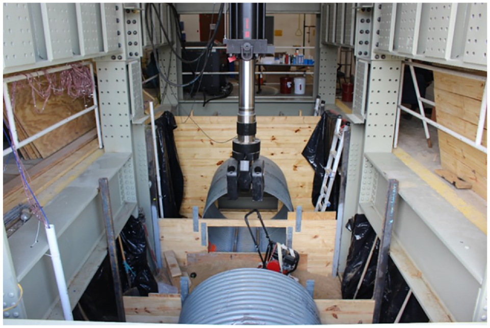
Soil box setup ( 8 ).

Geometry of The Soil Box

The soil box is 25 ft long, 11.97 ft wide, and 10 ft high (Figure 1). This is divided into three cells along the length using wooden partition walls. The wooden walls were braced at each end, and their stability under the application of the load was checked through theoretical methods, with each cell being about 7.97 ft long. To prevent the effect of soil-wall friction, lubrication was applied on wooden partition walls, and a layer of plastic sheet was placed in between the soil and all the partition walls and soil box surrounding walls. Any gaps between both ends of CMPs and partition walls were tightly sealed with Styrofoam. A 3300-kips MTS hydraulic actuator was installed to a steel reaction frame to load the buried CMP. The trench width of 11.97 ft agreed with the ( 17 ) recommendation that the minimum width of the trench should be greater than the maximum values of 1.5 times the outside pipe diameter plus 1 ft or the pipe outside diameter plus 1.33 ft. Meanwhile, the proposed trench width is consistent with ASTM D2321 ( 18 ) and BS 4660 ( 19 ), which state that the trench width should be at least 1.25 times the external pipe diameter plus 0.98 ft.

CMP Pipe

The corrugated metal culvert were 5(1/2) ft in length and 5 ft in diameter (Figure 2) with a thickness of 0.109 in. The corrugation profile was 2 2/3” × 1/2”. The pipe samples’ corrugated steel sheets conformed to ASTM Standard A929M ( 20 ) with yield strength 33 ksi and ultimate strength 45 ksi. The modulus of elasticity of the steel is 29,000 ksi. To represent the deterioration in the CMP, the CMPs were fabricated in a way that 18 in. of the entire invert could be removed after it was buried in the soil. The properties are listed in Table 1.

Figure 2.

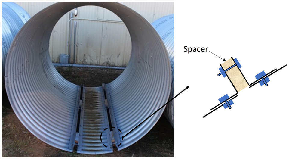
Photo of the corrugated metal pipe (CMP) pipe with the detachable part ( 8 ).

Table 1.

Properties of the Steel

Property	Value
Density (lb./in³)	0.284
Thickness (in.)	0.109
Corrugation size	2 2/3” × 1/2”
Moment of inertia (in⁴/in.)	3.425 × 10⁻³
Elastic modulus (psi)	29,000,000
Poisson’s ratio	0.3
Yield stress (psi)	33,000
Ultimate stress (psi)	45,000

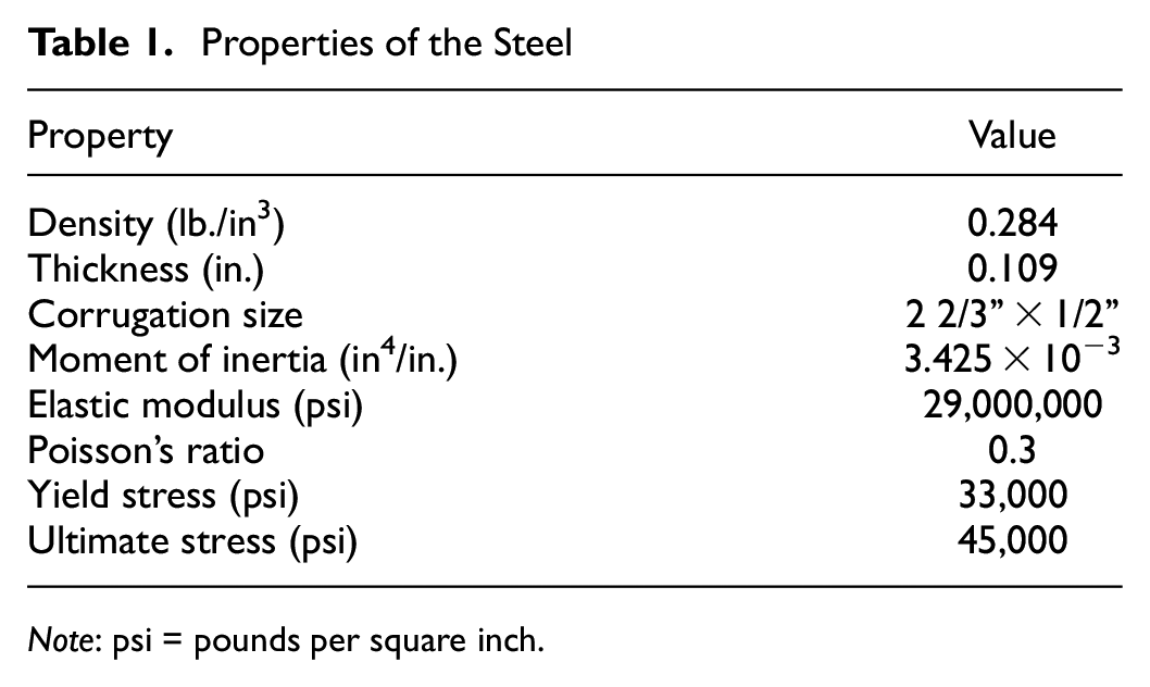
Note: psi = pounds per square inch.

Soil and Burial Configuration

A total of two types of soil were used to backfill the soil box. For the foundation and embedment layers poorly graded sand (SP) ( 21 ) was used, whereas for cover layer TxDOT classified Grade D subbase layer, which is also commonly referred to as recycled concrete aggregates (RCA), was used. Figure 3 shows the grain size distribution of the two soils. According to the unified soil classification system ( 21 ), the employed sand and gravel types are SP and poorly graded gravel (GP), respectively.

Figure 3.

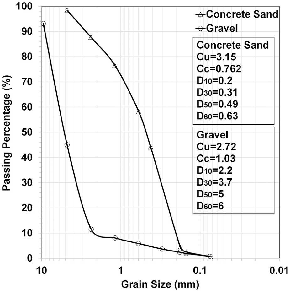
Grain size distribution of concrete sand and gravel.

The total depth of the soil box was 10 ft. The foundation was made of SP soil with a 2 ft depth and compacted to 95% compaction density, which was done based on ASTM Standard D698-12 ( 22 ). The foundation was followed by 6 in. bedding. The middle one-third of the bedding was loosely placed as per the recommendation from American Association of State Highway and Transportation Officials (AASHTO) ( 17 ) installation guide and then CMP was placed. It should be noted that the pipe embedded depth was 0.4D (D: pipe diameter). The fill height of the embedment was 5 ft and was placed with a lift thickness of 8 in. No compaction was applied on embedment as just placing the sand provided 85% proctor density. This compaction level was selected to represent a worst-case installation scenario where the soil is not compacted as expected, the compaction rate of 85% of SPDD was selected for embedment, and the 1 ft of SP backfill soil layers as specified by AASHTO ( 17 ). For concrete sand, the 85% compaction value can be achieved by only dumping and spreading the soil. In-situ compaction measurement using a nuclear density gauge showed the 85% compaction rate of SP soil can be achieved by dumping only. The same process was followed for backfilling the 2 ft cover. To prevent friction between soil and wall, lubrication was used on wooden walls, and a layer of plastic sheet was placed in between.

Polymer SAPL

The material property for this model was taken from the material test report provided by National Transportation Product Evaluation Program (NTPEP). The test report of the NTPEP ( 23 ) liner had a maximum of 1.5% elongation before the crack. The test report suggested the brittle behavior of the material with a small plastic zone with only 0.22% strain difference between the yield and breaking strain. Based on the report, the liner’s physical characteristics are presented in Table 2. After completing the backfilling of the CMPs, three different liner thicknesses (0.25, 0.5, and 1 in.) were applied to renew the three pipes. In the invert section, direct spraying on the soil was not feasible. Consequently, the detached invert section (middle section) was left in place to accommodate the liner. A 2-in. gap existed between each side of the invert section and the primary CMP body. These gaps were filled with Styrofoam, covered with plastic sheets, and sealed with duct tape. The application of the SAPL was carried out manually. To control the thickness during installation, the volume of sprayed material per unit of time (i.e., seconds) was used to estimate the amount of material applied to the interior surface of the CMPs each second. Additionally, knowing the total volume required for SAPL, the number of passes needed to achieve the desired thickness was estimated. Subsequently, the thickness of the installed SAPLs was measured using an OLYMPUS 38DL PLUS^® Ultrasonic thickness gauge. Measurements were taken at three locations longitudinally along the length of the pipe and at 45° intervals circumferentially. Owing to the probe’s size, measurements were taken on the crest of the corrugations at the designated locations. Three measurements were recorded at each point, and the average thickness value for that location was documented. The results revealed that the thickness was uniform, and the maximum discrepancy error was less than 20%.

Table 2.

Properties of the Liner ( 23 )

Property	Value
Density (lb./in³)	0.00014
Elastic modulus (psi)	1,154,016
Poisson’s ratio	0.3
Tensile yield stress (psi)	7,482
Tensile yield strain (%)	1.13
Tensile break strength (psi)	8,228
Tensile break strain (%)	1.35

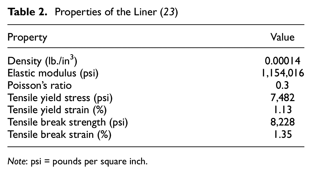
Note: psi = pounds per square inch.

Instrumentation

The CMPs were instrumented thoroughly using instruments such as LVDTs, CDSs, uniaxial strain gauges, and earth pressure cells ( 6 , 24 ). Three cameras were placed inside the pipe during testing to monitor the continuous change in the CMP profile during the load application. Three LD620-150 LVDTs from OMEGA were placed inside the CMP to record the horizontal and vertical displacement at crown, shoulder, and springline. To implement LVDTs inside the pipes, a frame to hold the sensors was required. The frame was designed to not touch the testing specimen because doing so might skew the results. The frame has been cantilevered inside the pipe to support the sensors. The configuration of the LVDTs and CDSs sensors inside the CMP is shown in Figure 4a. The instruments implemented inside the pipe were attached after backfilling and spraying the liner inside the pipe.

Figure 4.

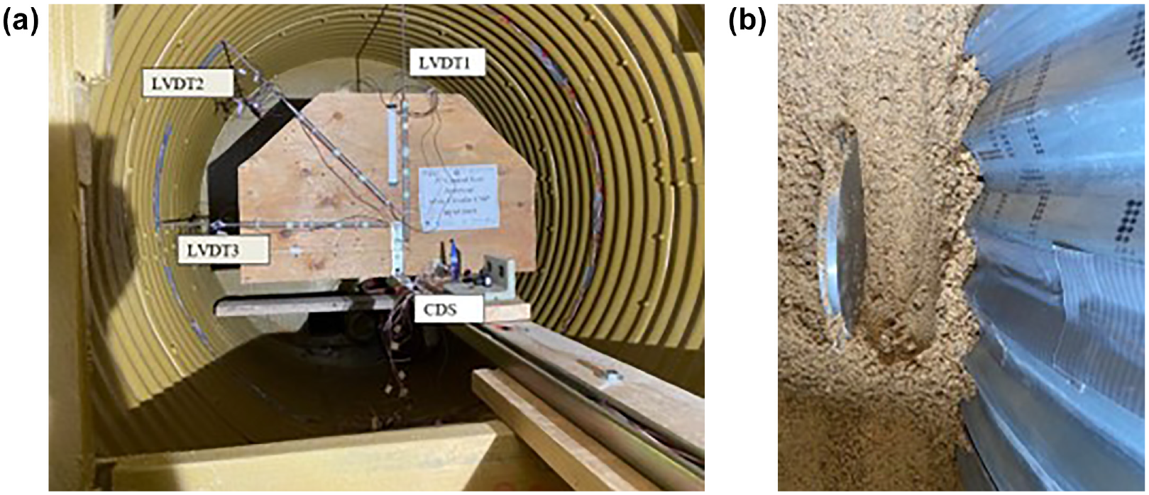
Instrumentation for the tested corrugated metal pipe (CMP): (a) linear variable transducers (LVDTs) and cable displacement sensors (CDS) arrangement and (b) earth pressure cell at spring line ( 8 ).

Four earth pressure cells installed during the backfilling process were used to measure the increase in pressure during the application of the load. The earth pressure cells were placed at the invert, on both sides of spring-lines and at the crown as shown in Figure 4b. All the earth pressure cells were placed 4 in. away from the CMP to eliminate the point load effect on the sensors provided owing to the corrugated shape of the CMPs.

The strain in the CMP were measured using 16 uniaxial strain gauges, model C2A-06-250LW-120 from Micro-Measurements, around the CMPs in the direction of the hoop stress under the center of the loading plate and the most critical region ( 25 ). The nomenclature of the strain gauges is presented in Figure 5 (e.g., C1-C AND C1-V strain gauges at the crest and valley) by considering the and same nomenclature are followed for all the data analysis after this. The strain gauges at the pipe’s crest were attached to the pipe’s outer surface, and the strain gauges at the valley positions were also attached to the SAPL’s outer side as shown in the Figure 5b. Based on the attachment preparation process, cabling, and the probable impact of the spraying coating layer on strain gauge performances, the inner pipe strain gauges were attached to the SAPL’s outer side.

Figure 5.

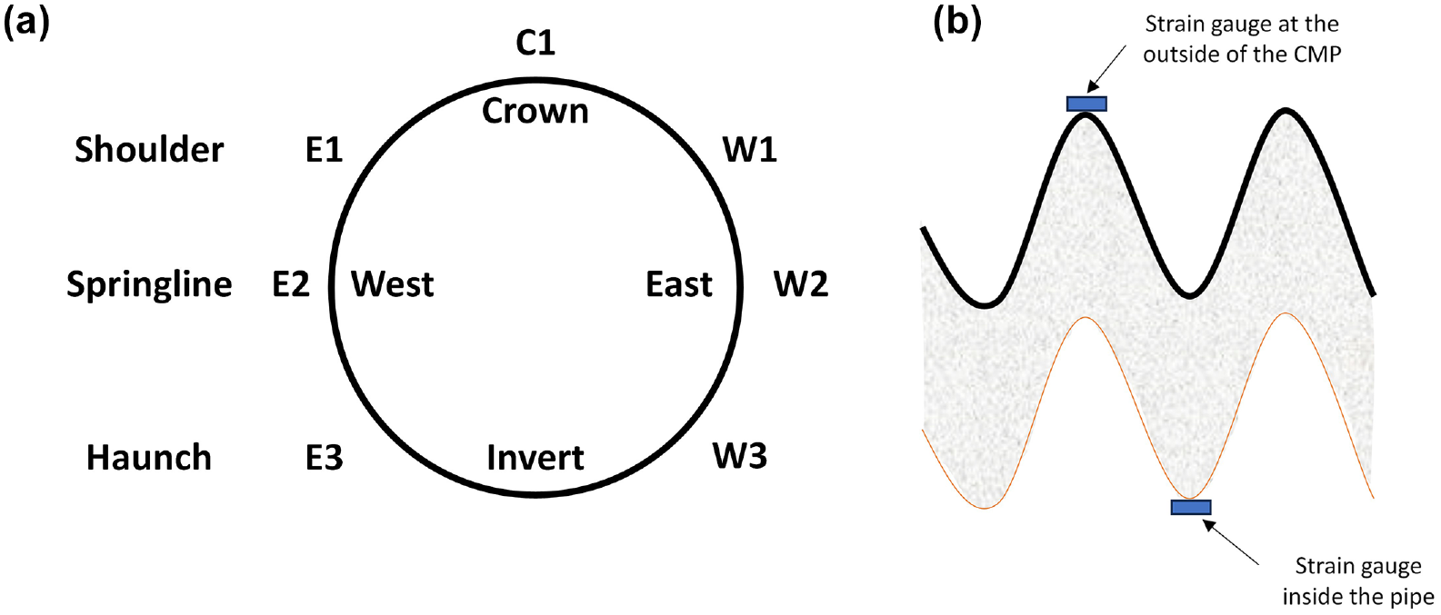
Strain gauges, (a) location of the placement of strain gauge along the circumference (b) arrangement of strain gauge in corrugated metal pipe (CMP) and liner.

Loading Configuration

According to AASHTO ( 17 ), the load through a vehicle on the pavement is transferred as uniform stress over a rectangular area equal to the contact area of the wheels ( 25 , 26 ). Thus, the test was carried out for H20 truck with a service load of 16 kips from each wheel load. Since, for an H20 truck, the contact area will be 10” × 20” thus it was decided to choose the load pad size of 10” × 20”. But during the control tests it was observed that load pad punched through the soil and failure of the soil was observed before the failure of the pipe which was not desirable condition for our test ( 6 ). Therefore to prevent the failure of the soil before the failure of the CMP the smaller load pad of size 10” × 20” was replaced by the load pad of the size 20” × 40”. The load in the soil box system was provided through a hydraulic actuator that was installed to apply the load. The CMP samples were loaded using a 330-kip MTS hydraulic with the loading rate of 0.03 in./min, and the actuator attached to a reaction steel frame being installed inside the soil box to support the actuator located at the CUIRE laboratory.

Finite Element Model

Model Setup

Previous studies have shown that considering a 2D or equivalent 3D FEM model of the CMPs would affect the results from the FE results ( 5 , 11 , 12 ). Thus, a full 3D model of the soil box, CMP, and liner was generated using CAD software and was imported to ABAQUS. The boundary conditions in the models were defined according to the experimental setup. All the vertical soil faces were defined as restricted in their normal directions and free in their tangential directions. The vertical movement of the soil was restricted on the bottom surface.

Material Model

Soil Properties

Two types of soil, poorly graded sand (SP) and TxDOT-specified Grade D sub-base layer were considered as the backfill and cover soils, respectively, in the experiment. The Drucker Prager model was used to model the soil in the FEM model. Drucker Prager model is a 3D pressure-dependent model through which the strength properties of the soil increased with the application of the pressure ( 27 ). The property of the poorly graded sand was taken from the laboratory experiment carried out at the Geotech lab of UTA by using some triaxial compression tests on moist samples. The triaxial compression tests on moist samples (equivalent to 92% relative density and 3% moisture content) revealed that the internal friction angles (Ø) for sand and gravel were 32° and 37°, respectively. The cohesion values for the soil types were literally zero. The Young’s modulus for the soils was also determined from the loading-settlement figures based on the preliminary plate load tests. In the calibration process, the internal friction angles of the sand and gravel were adjusted slightly to better match the experiment results. The properties shown in Table 3 are the finalized values after the calibration process.

Table 3.

Soil Properties

Property	Sand	Recycled concrete aggregates
Density (pcf) (max. dry density)	115	130
Young’s modulus (psi)	510	1,000
Poisson ratio	0.3	0.3
Angle of friction	32.0	39
Dilation angle	1	1

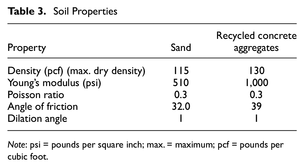
Note: psi = pounds per square inch; max. = maximum; pcf = pounds per cubic foot.

CMP and Liner Properties

The simple elastic-plastic model available in ABAQUS was used to model the behavior of the CMP steel pipe and the liner. The properties are listed in Tables 1 and 2 for the pipe and liner accordingly. The occurrence of the crack is identified by observing the plastic strain in the liner as it has lower yield strength than the pipe. Since the liner had a small plastic region, the occurrence of the first plastic strain was related to the occurrence of the first crack in the model.

Mesh Sensitivity

Mesh sensitivity analysis was reported by Chimauriya ( 6 ) for this FE model. To determine the mesh sensitivity of the model, total energy, load-displacement for soil and pipe, and the von Mises stress for the pipe were compared. For the soil, three different mesh sizes, 3.4, 3, and 2.4 in., were taken into consideration for mesh size study, whereas for the CMP and liner, mesh sizes varied from 2.4 to 0.75 in. The final mesh size of CMP and liner was 1.8 ( 6 ). For soil, a mesh size of 2-in. was used around the vicinity of the CMP, and a mesh size of 4-in. was used away from CMP. A mesh size of 2-in. was used in the vicinity of the liner to make the mesh of soil compatible with the mesh size of CMP. Coarser mesh sizes were used away from the CMP to reduce the computational time ( 5 , 11 ). The distribution of the mesh is shown in Figure 6.

Figure 6.

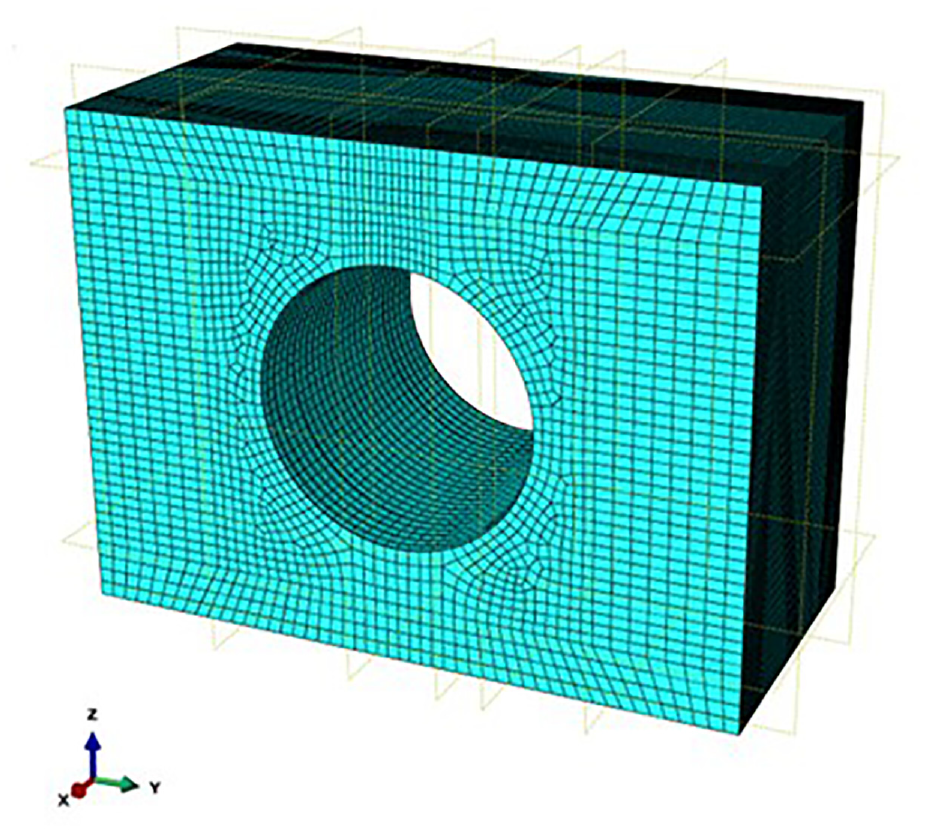
Distribution of mesh in the soil box.

For all the models, the same element type was used. A linear C3D8R element type was used in the model, which can be defined as 8-node linear brick elements with reduced integration and control in the hourglass.

Soil–Pipe and Pipe–Liner Interactions

ABAQUS allows users to define different interaction models of the interface between the pipe and soil, for example tie interaction and surface-to-surface interaction. In previous literature, the interaction between soil and CMP was represented using the tie interaction ( 3 , 5 , 11 , 28 ). However, owing to the removal of the invert, the soil and CMP moved independently, which could not be represented using tie interaction. Thus, the interaction between the pipe and soil interface is represented using the surface-to-surface contact model where the pipe was treated as the master surface and the soil was treated as the slave surface. This contact was chosen to simulate actual physical tests in which pipe-to-liner slippage was possible. Considering the corrugated surface of the pipe, a rough friction coefficient of 0.5 with the hard-normal contact was defined between the CMP and soil. This friction coefficient was the optimized value as the result of calibrating the FE model with the test results.

The same contact model was used to model the CMP and liner interactions, but a larger friction coefficient of 1.0 was used to represent a stronger tangential bonding. Post-test observations showed a separation of the liner from the pipe at the location of failure; therefore, zero normal bonding strength was applied in the interaction model.

Model Step

The model steps followed to obtain results from the FE model are described below.

STEP 1 Geostatic step: In this step, geostatic (in situ) stresses including vertical and horizontal stress were established for the soil domain without considering the CMP pipe. In this step, we deactivated the pipe, but we restricted the pipe tunnel displacement. It should be noted that the entire soil heights model is performed in one step. The vertical stresses were calculated using Equation 1, while the lateral stresses were calculated as in Equation 2.

σ = γ H

(1)

σ_{h} = (1 - \sin φ) γ H

(2)

STEP 2 Installation of CMP: The deactivated CMP was activated in regards to defining the interactions between the pipe and the surrounding soil. In this step, the gravity load of the pipe was activated, and pipe–soil interaction was established by removing the restrictions applied to the inner tunnel surface of the soil.

STEP 3 Removal of the invert: In this step, we performed a specific operation by removing the invert of the CMP. The invert refers to the lower part section of the pipe. By removing this section, we are essentially altering the model to reflect a change in the pipe’s geometry or configuration.

STEP 4 Installation of the liner: The liner model was activated, and the pipe–liner contact was activated to establish the liner-CMP interaction.

STEP 5 Load application: Application of the load on top of the 1 ft cover was initiated by defining load displacement of 0.03 in./min. based on replication experimental tests.

Concerning the model’s resemblance to experimental tests, where measurement and analysis began after instrumentation and backfilling, the backfilling and pipe placement phases were disregarded.

Results and Discussion

Although the polymer was brittle and its failure mode was expected to be cracking of the liner (about 0.22% strain difference was seen in the tensile yielding and the breaking point), the liner is modeled using the simple elastic-plastic model. When plastic strain is developed in the liner, it is considered as the crack observed in the physical test. This is a pseudo approach as opposed to the modeling of the crack initiation and propagation in the FEM modeling. Thus, the appearance of the first crack in the experiment was related to the appearance of the first plastic strain in the model. Overall, it was found that the model was close in predicting the first crack through the first plastic strain concept. The FE model results for 0.25, 0.5, and 1 in. SAPL thicknesses are verified with the experimental results. This verification ensures the parametric studies in which we discussed the role of the stiffness of the liner, friction angle between the liner and the pipe, buried depth of the pipe, and different thicknesses of the liner.

Model Verification

The results showed that the liners’ responses in the FE models compared well with the experimental results. In the test for the liner with a thickness of 0.25 in., it was observed that the first crack occurred at the center of the CMP at the crown region. In the FEM model, the first plastic strain was exactly seen at the center of the CMP at the crown region (Figure 7). The plastic strain experienced in the crown propagated longitudinally along with the crown of CMP in the FE model, which matches well with the propagation of the crack in the experimental results (Figure 7). For the CMP pile with the 0.5 in. SAPL thickness, same as the one with 0.25 in. thickness, the plastic strain appeared first at the center of the crown and then propagated longitudinally at the crown line when the load peaked. In addition, no significant plastic strain was seen on the other locations of the liner.

Figure 7.

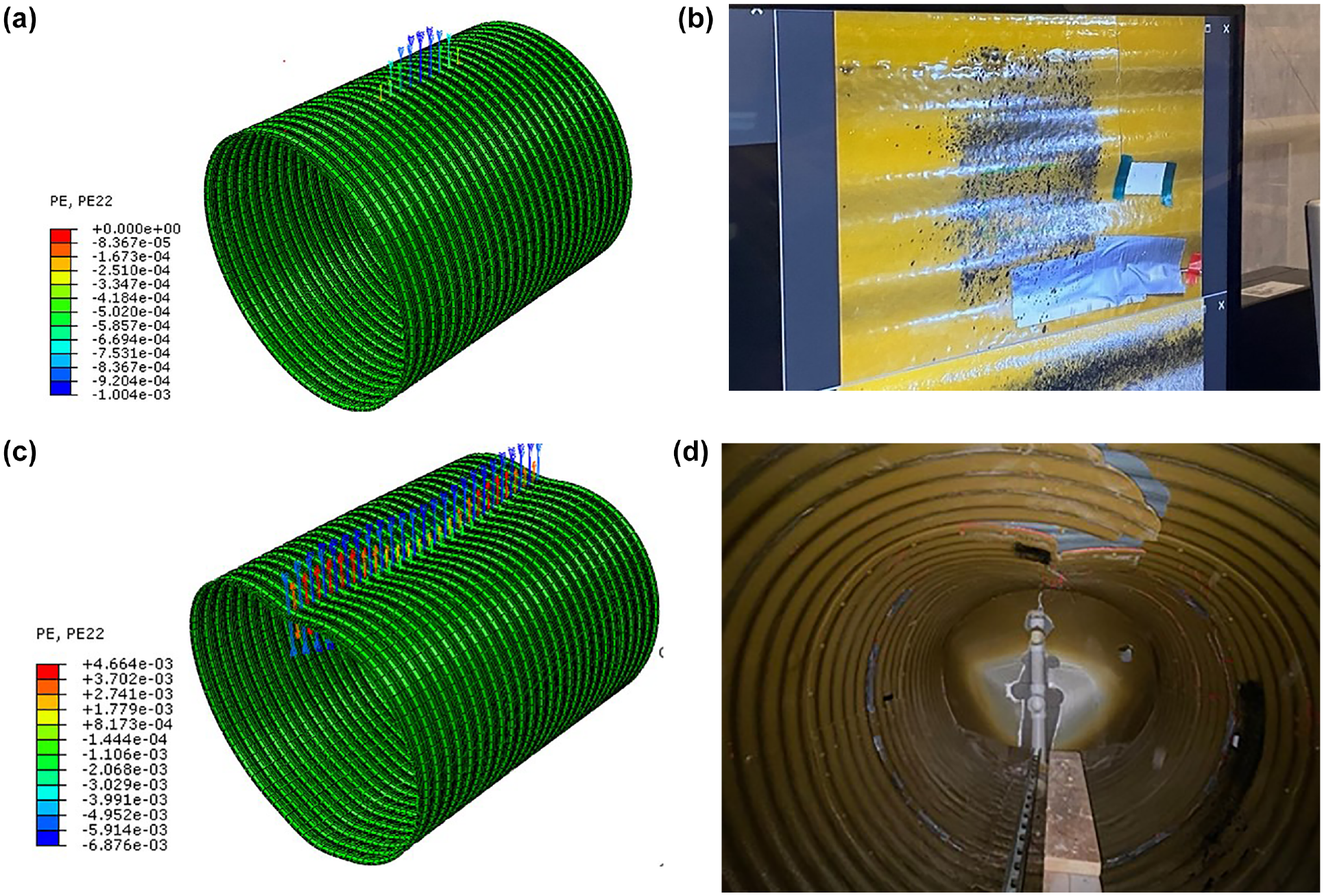
Comparison of plastic strain in finite element (FEM) and crack from visual observation: (a) first plastic strain in the FE corrugated metal pipe (CMP), (b) first crack in the test for 0.25 in. thick liner ( 8 ), (c) plastic strain at the ultimate load in the FE model, and (d) crack in the liner at the end of the test for 0.25 in. thick liner (Z = 0.4D) ( 8 ).

The FE model for 1 in. thick SAPL also compares well with the experimental results. The first plastic strain was seen exactly at the center of the CMP at the crown region. After that, the plastic strain in the FE model propagated along the top centerline of the pipe in the FEM, similar to the observed experiment results.

Verification of Load Displacement

The displacement of the CMP and the liner were monitored at the crown, spring line, and shoulder using the LVDTs in the experiment. The comparison showed very similar results and the average discrepancies between the experimental and numerical results is less than 7% (Table 4).

Table 4.

Comparison of the Load and Displacement between the Finite Element Model (FEM) and the Experimental Results for Different Line Thickness

Description	First plastic strain	First crack	Discrepancy test versus FEM (%)	Ultimate load		Discrepancy test versus FEM (%)
Description	FEM	Test	Discrepancy test versus FEM (%)	FEM	Test	Discrepancy test versus FEM (%)
Liner thickness: 0.25 in.
Vertical crown displacement (in.)	3.13	2.92	6.7	4.92	5.23	5.92
Soil surface displacement (in.)	4.86	4.64	4.7	6.0	6.49	7.5
Load (kips)	43.5	41.3	5.3	45.63	45.78	0.3
Springline disp. (in.)	0.68	0.86	20.0	0.95	1.14	16.6
Liner thickness: 0.5 in.
Vertical crown displacement (in.)	2.37	2.18	8.01	4.72	4.74	0.42
Soil surface displacement (in.)	3.36	3.02	10.11	6.49	6.09	6.16
Load (kips)	42.30	42.59	0.68	50.15	52.24	4.0
Springline disp. (in.)	0.54	0.60	10	0.98	1.15	10
Liner thickness: 1.0 in.
Vertical crown displacement (in.)	2.74	2.36	11.65	3.85	4.16	7.4
Soil surface displacement (in.)	5.5	4.9	10.90	8.0	7.4	7.5
Load (kips)	67.10	66.26	1.25	70.2	72.17	2.7
Springline disp. (in.)	−0.82	−0.70	12.63	−0.99	−1.02	2.9

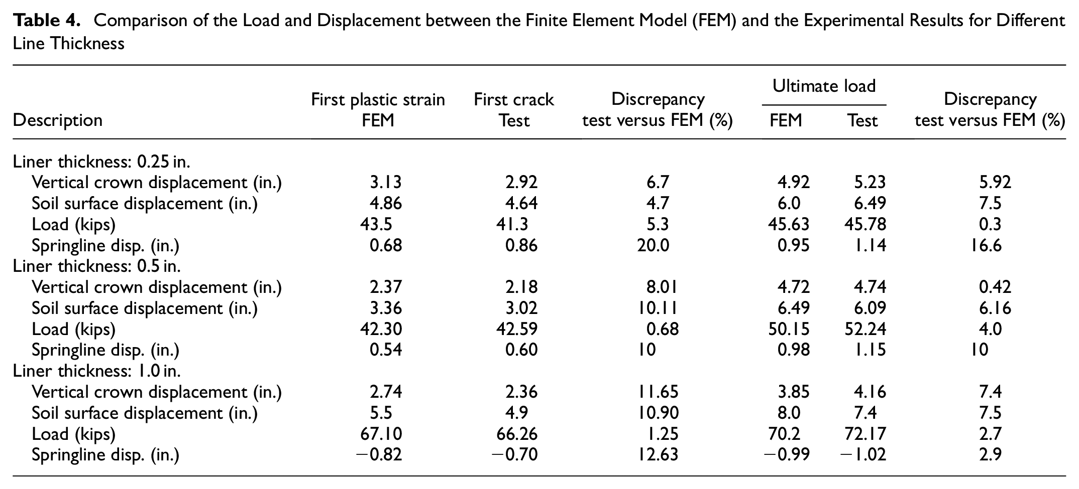
In the test, owing to over spraying of the polymeric liner material, the CMP was attached to the boundary wall by the over-sprayed liner, which increased the initial stiffness of the liner. However, this attachment was not able to be practically modeled in the FE model. For example, in the 0.25 in. liner, the corresponding load for the yield point in the FEM was around 43 kips, which had a discrepancy of 6% in comparison with the appearance of the first crack in the test (Figure 8). In addition, the liner pipe system took the peak load of 46 kips in the test, which was predicted to the accuracy of 0.3% by the FE model. In the case of 1 in. liner, owing to the increased thickness in the liner, the attachment to the wall was also thicker and it only got separated at the time of the occurrence of the first crack in the experiment. During the first crack and complete separation of the liner from the wall, there was a large drop in the load, but such a drop was not observed in the FEM as FEM was modeled in the ideal case scenario; that is, no attachment to the end wall (Figure 9). Figure 9 also shows the load–displacement results of the numerical analyses against the experimental ones at the soil surface, crown, shoulder, and springline regions. The results show the employed numerical approach could adequately model the experimental tests.

Figure 8.

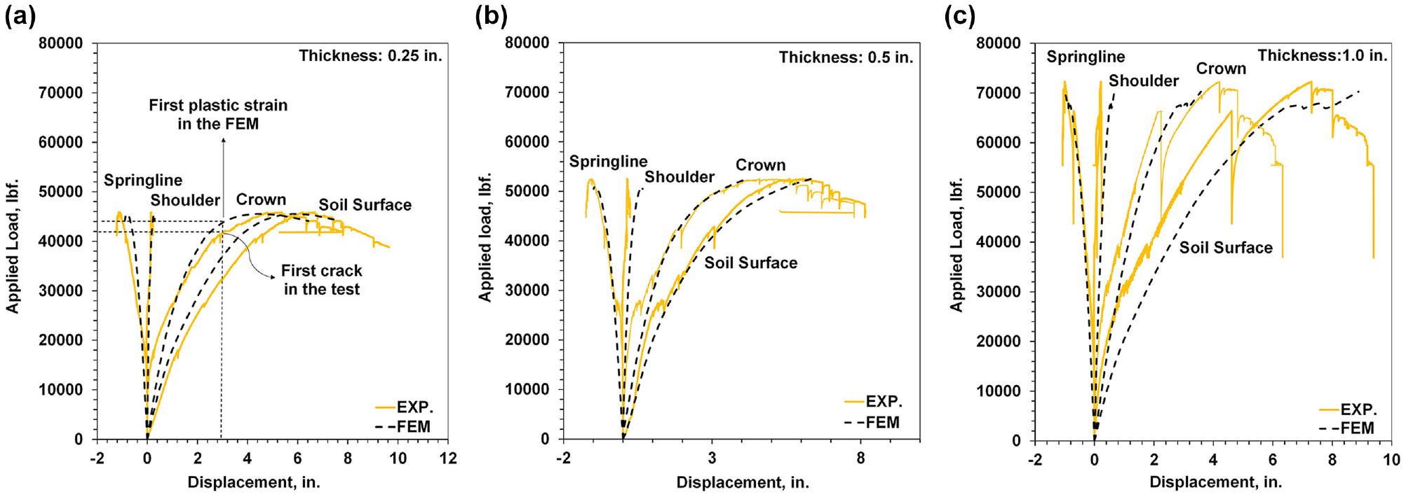
Experiment and finite element (FEM) results of applied load versus soil surface settlement and liner displacements at crown, spring line, and shoulder for different liner thicknesses: (a) 0.25, (b) 0.5, and (c) 1.0 in.

Figure 9.

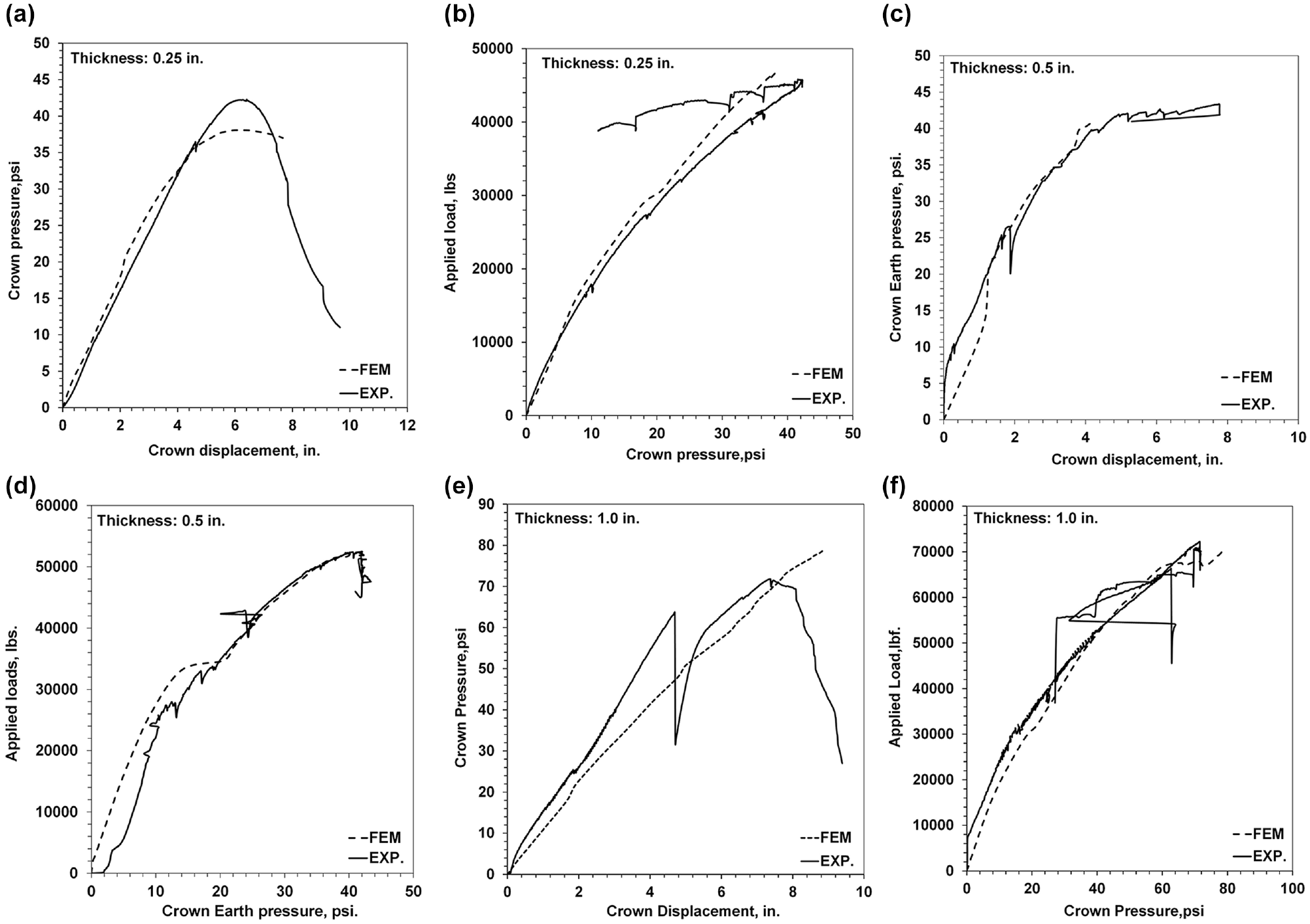
Verification for the crown pressure against the crown displacement and the applied load for different liner thicknesses of (a, b) 0.25 in., (c, d) 0.5 in., and (e, f) 1.0 in.

Verification of Pressure and Displacement

The earth pressure in the crown would give the actual amount of pressure that can be taken by the liner to crack and reach the peak load. The earth pressure readings were taken from the earth pressure cell placed at 4 in. away from CMP in the crown, springline, and invert. For the FEM, the comparisons of the earth pressure were made only at the crown as the earth pressure at the spring line, and invert was low compared to the crown. The pressure plots showed a similar pattern of the curve for the experimental and the FE model results (Figure 9). The earth pressure at the time of the first crack and the appearance of the first plastic strain of the liner were nearly equal.

In the 0.25-in.-thick liner, the earth pressure at the occurrence of the first crack was measured as 36.42 pounds per square inch (psi) when the liner displacement reached 2.92 in. during the experiment. However, in the FE model, the earth pressure was recorded as 36.16 psi at the moment of the first plastic strain with a liner displacement of 3.13 in. Note that at the ultimate conditions the FE model seems to take less load than the experimental condition. This is attributed to the perfectly plastic definition of the material. Once the material yields, it can no longer take the load. The ultimate crown pressure showed a discrepancy of about 7% between the experimental and FE model results. For the liners with 0.5 and 1-in. thicknesses, the comparison of the liner displacement and the earth pressure at the crown shows the same trend between FE and test results. Also, the comparison of the applied load and earth pressure at crown follows the same curve for FEM and test results as shown in Figure 9.

Verification of Strains

The data logger was damaged for the tests (0.25-, 0.5-, and 1.0-in. liners), and the data could not be fully recovered. As some of the data were recovered, the comparison of the strains was made in the crown and the shoulder region only for 0.25-in. and 1.0-in. liners. The obtained results for the liner were plotted against the soil displacement. Concerning the 0.25-in. liner, the strains at the crown, located outside in the crest of the CMP, were overestimated compared to the experimental results. The strain recorded from the strain gauge located outside of the CMP in the crest in the shoulder matched well with test results (Figure 10a). Although the comparison of the strains was fair for the strain gauge located on the outside crest in CMP, the strains that were recorded from the strain gauge located on the inside crest of the liner did not match. These discrepancies might be caused by issues related to the datalogger, strain gauge attachment, and the manner in which the liner was affixed to the pipe during the tests. Furthermore, the friction model employed between the pipe and liner in our numerical simulations may not capture the complete extent of slippage, unlike what is observed in the experimental setup. As a result, differences between the experimental and numerical analyses become more evident as slippage reaches a certain threshold. Lastly, as previously highlighted, variations in liner thickness within the pipe body could also contribute to the variations observed between the experimental and numerical results. With regard to the 1.0-in. liner, the predicted strain till the first crack in the test and the FEM followed the same path (Figure 10b). After the crack, the FE and test results showed the variation. The slope of the strain changed immediately after the crack, but the slope did not change for the FE results, which suggests that the liner loses its strength capacity once the crack is formed in the liner, and this loss in capacity of the liner after the appearance of the crack is not predicted by FEM. Overall, FEM predicted the strains well before the appearance of the first crack in the test.

Figure 10.

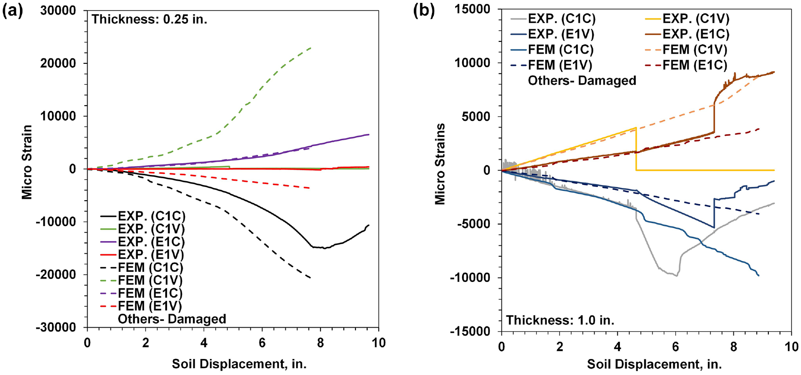
Comparison of the measured and simulated strains and for different liner thicknesses: (a) 0.25 in. and (b) 1.0 in.

Parametric Study

In the previous sections, the laboratory behavior of the buried pipes was verified by numerical analyses. The results showed that the applied constitutive approach and the parameters of the numerical analyses can model the behavior of the pipes with acceptable accuracy. Based on the verified model, the behavior of buried invert-cut CMP pipes is further analyzed in four different situations. The analyses help to evaluate the behavior of buried CMP pipes in different settings. Three distinct test types were employed. First, the effect of increasing the embedment depth was explored with burial depths of 0.4D, 0.7D, and 1.0D while maintaining a constant liner thickness of 1 in. Secondly, the influence of altering the liner’s elastic modulus was investigated by considering a 25% and 50% increase in the elastic modulus of the liner, with the liner thickness held at 1 in. and the burial depth fixed at 0.4D. Finally, the analysis delved into variations in the liner’s thickness, focusing on thicknesses of 0.25, 0.5, 1.0, and 1.5 in. while maintaining a consistent burial depth of 0.4D. These parametric studies aim to provide insights into how burial depth, liner thickness, and liner elastic modulus affect the behavior on sprayed CMP pipes.

Burial Depth

One of the influencing factors on the behavior of buried pipes is their buried depth ( 25 , 26 , 29 ). The volume of energy-absorbing layer (soil) between the loading surface and the buried pipe increases by increasing the burial depth. In this situation, by considering the same amount of displacement from the surface, less settlement in the buried pipe could occur. Figure 11 shows the circumferential deformation values of the buried pipes in all three mentioned burial depths. The figure indicates the major pipe deformations have occurred in the crown region, and the deformation in other areas can be ignored in comparison with the crown displacement. The amount of the crown deformations is equal to 5.6, 3.6, and 2.3 in., respectively, for the Z = 0.4, 0.7D, and 1.0D. As it is known, with increasing the burial depth of the pipe to 0.7D, the maximum deformation of the pipe has decreased by about 31%. This value reached 58.9% with increasing the burial depth of the pipe to 1.0D. With regard to the horizontal deformation, the values of deformations in the corresponding states are equal to 2.01, 1.32, and 0.79 in., respectively, for the Z = 0.4, 0.7D, and 1.0D embedment depths. The horizontal deflection of the buried pipes decreased on average by about 50% by increasing the burial depth from 0.4D to 1.0D.

Figure 11.

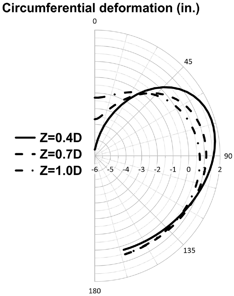
The amount of circumferential deformations of the pipes in different situations (liner thickness = 1 in. and 10 in. surface displacement).

Figure 12 illustrates the distribution of stress within the backfill and pipe under the same stress level. It is well-established that when the burial depth decreases, the force applied to the surface of a pipe can intensify, given that the force is concentrated over a smaller area. Consequently, this increased force results in a higher rate of deformation for the pipe.

Figure 12.

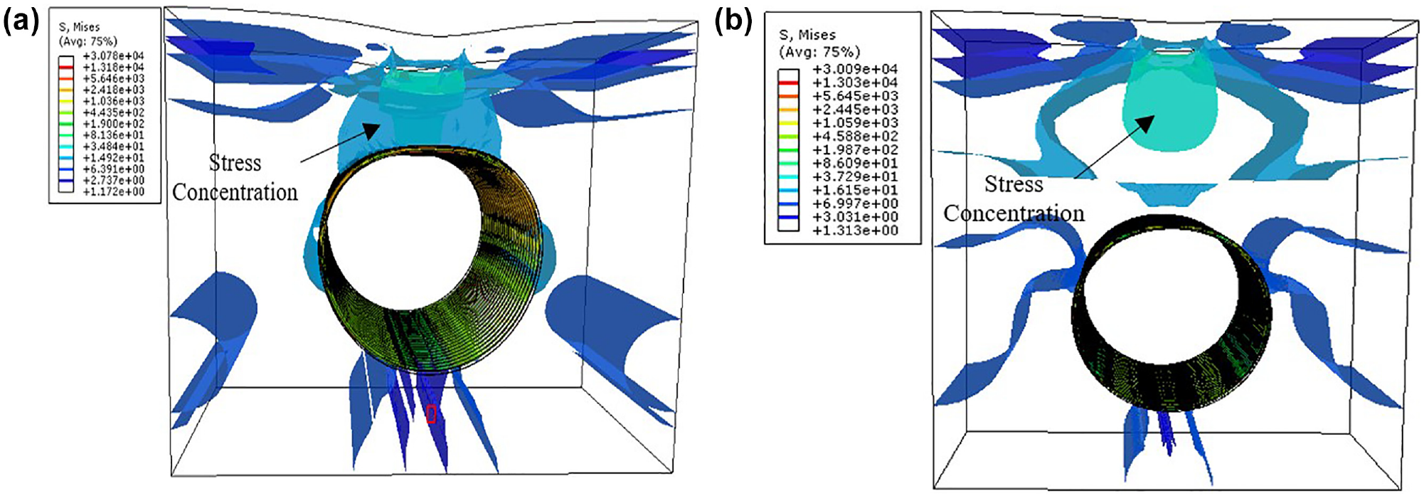
Stress propagation in the backfill and pipe assembly: (a) Z = 0.4D and (b) 1.0D.

Longitudinal strain is one of the vital factors that can affect the behavior of buried pipes ( 25 ). Figure 13 shows the deformation of the buried pipes at the side and crown of them along their lengths. The results show that by increasing the burial depth of the pipes, the amount of longitudinal deformation of the pipes would decrease. For example, when increasing the burial depth of the pipe from 0.4D to 1.0D, the difference in the crown deformations between the crown and tips of the pipe decreased from 0.761 in. to 0.021 in. This decrease indicates a reduction of about 97.2% in the amount of longitudinal strain values at the crown region. This amount of reduction in the longitudinal strain of pipes can be very useful in ensuring the serviceability of the buried pipes. Another noteworthy point is that with increasing the burial depth of the pipe, the deformation values would decline in all areas of the pipe, so that in the springline region, with increasing the buried depth, the horizontal deformation of the pipe has decreased sharply.

Figure 13.

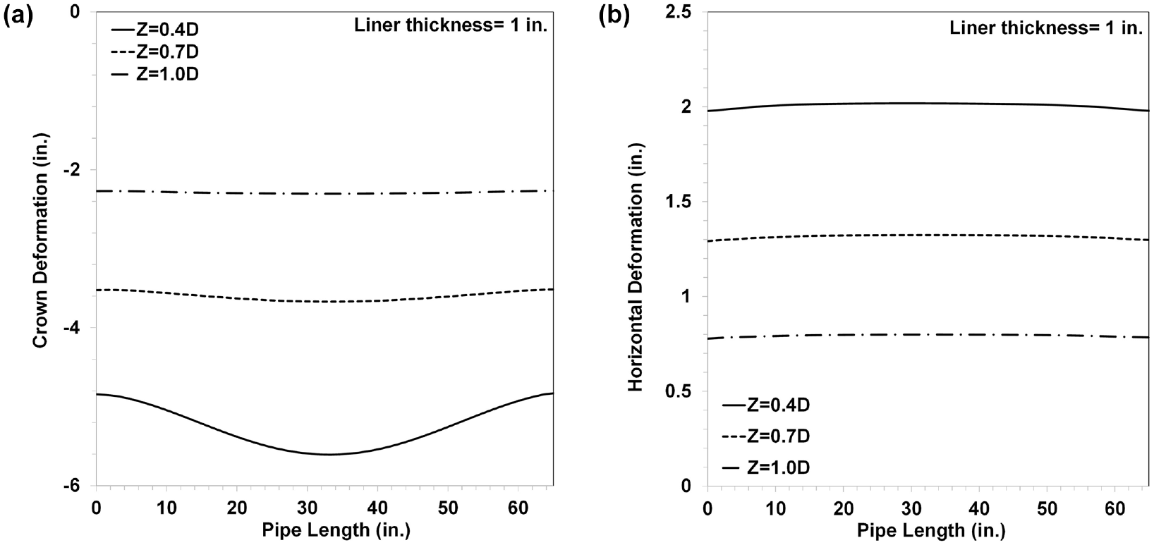
Deflections along the length of buried pipes: (a) the maximum pipe crown displacement and (b) the maximum pipe springline displacement (liner thickness = 1 in. and 10 in. surface displacement).

Assuming a linear distribution of the strain, the circumferential bending moment and thrusts at different locations in the CMP were calculated by using the strain from numerical analyses at the crest and the corresponding valley as follows (Elshimi [ 11 ]):

M_{θ} = \frac{E I_{θ} (ε_{crest} - ε_{valley})}{d}

(3)

where M_θ = circumferential bending moment (lbf-in./in.), I_θ = moment of inertia per unit length in the circumferential direction (in.⁴/in.), $ε_{crest}$ = circumferential strain measured at crest of the corrugation, $ε_{valley}$ circumferential strain measured at valley of the corrugation, d = depth of corrugation (in.), and E = modulus of steel (lbf/in.²).

N_{θ} = \frac{E A_{θ} (ε_{crest} + ε_{valley})}{2}

(4)

where N_θ = circumferential thrust (lbf), A_θ = cross-section area per unit length in the circumferential direction.

Figure 14 depicts the distributions of circumferential thrust and bending moment around the CMP pipes at the center of the pipes and at the end of the analysis (10 in. surface displacement). The results show the most sensitive region is the area between the crown and shoulder ( 30 ). The results show that the most sensitive area is between the crown and the shoulder ( 30 ). The results show that increasing the burial depth of the CMP pipes from 0.4D to 1.0D reduces the maximum thrust and bending moment at the pipe’s crown by 83% and 78.5%, respectively. The thrust and bending moment results also show that as the burial depth increases, the corresponding values in the shoulder area can decrease, whereas the values in the spring line area are literally equal. The high burial depth pipes perform the best in this regard.

Figure 14.

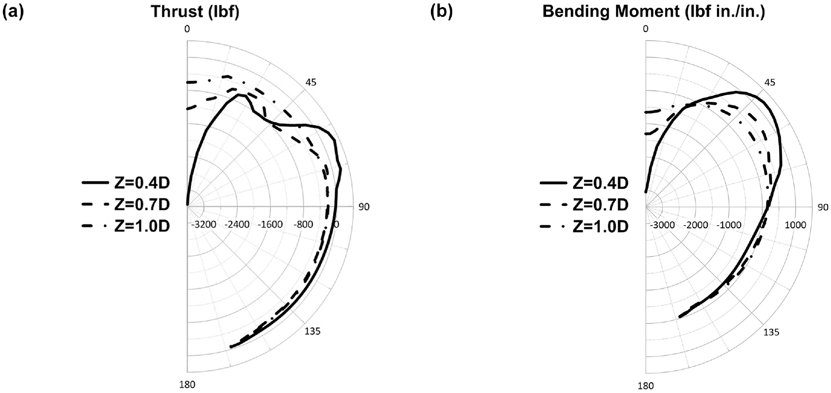
Simulated corrugated metal pipe (CMP) using the finite element (FE) model (liner thickness = 1 in. and 10 in. surface displacement): (a) circumferential thrust and (b) bending moment distribution.

Elastic Modulus of the Liner Layer

In this section, by considering the constant thickness of 1 in. for the liner layer and embedment depth of 0.4D for the pipes, the elastic modulus of the liner has increased by 25% and 50%, respectively. Figure 15 shows the extent of the circumferential deformations of the pipes in three different states. As it is known, with increasing the elastic modulus of the liner by 25%, the maximum vertical and horizontal deformation of the pipe has decreased only by 7% and 3.5%, respectively. By increasing the elastic modulus to a value of 50%, this value has reached 8.9% and 6.2%, respectively. These values indicate that increasing the elastic modulus of the liner layer couldn’t have much effect on improving the behavior of the pipe. Also, concerning the amount of vertical and horizontal deformations of the pipe along its length (Figure 16), with increasing the elastic modulus of the liner layer by 50%, the maximum amount of vertical deformation of the pipe crown between the center and side has decreased by about 30%. This value is about 35% in the springline area of the pipe. It is important to note that with increasing burial depth of the pipe, the maximum reduction amount has been about 97%.

Figure 15.

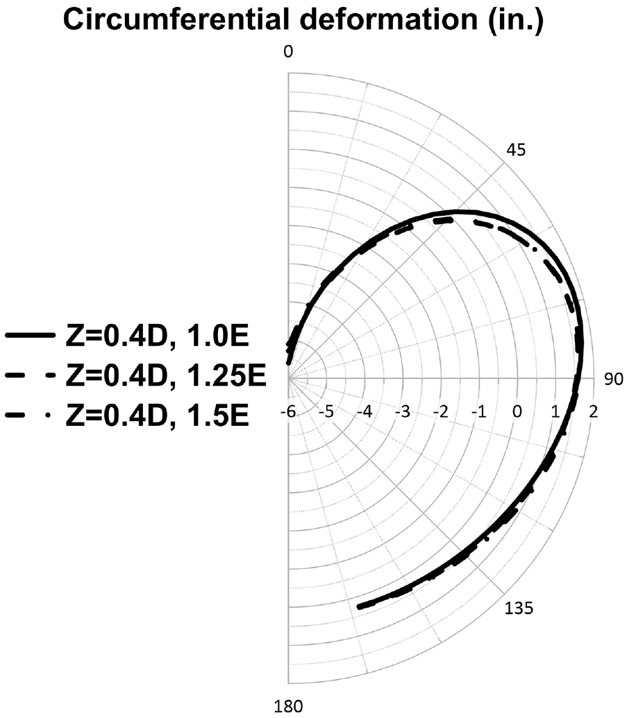
The amount of circumferential deformations of the pipes in different situations (liner thickness = 1.0 in.).

Figure 16.

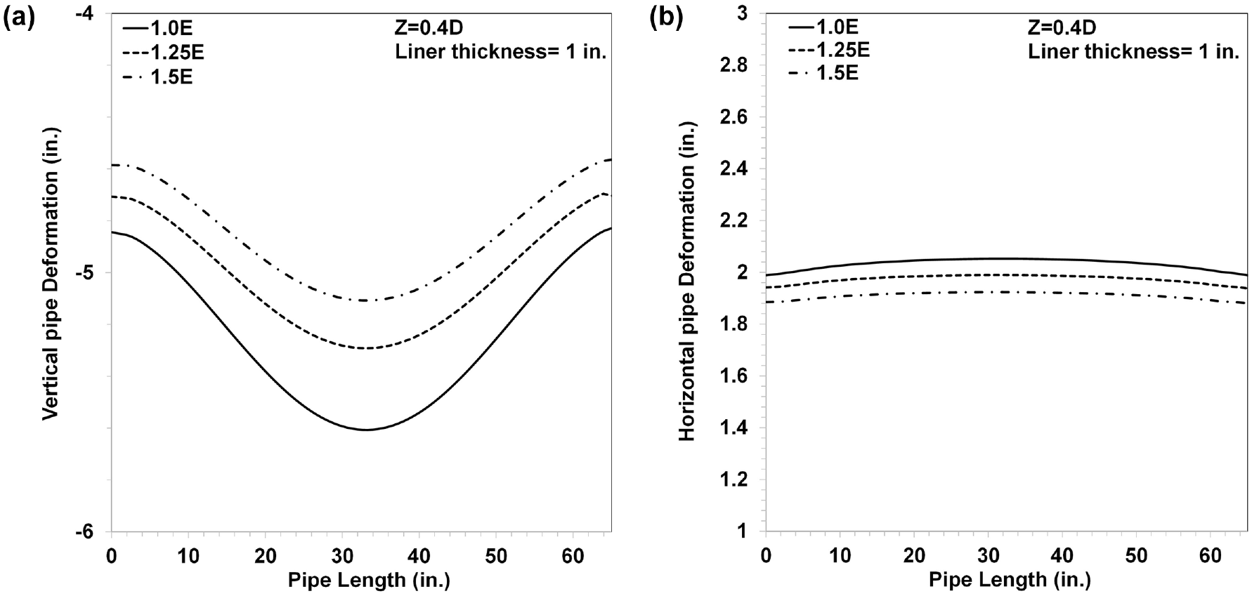
Deflections along the length of buried pipes: (a) the maximum pipe crown displacement and (b) the maximum pipe springline displacement.

It can be seen that the repaired pipes have little improvement due to the increase of liners’ modulus. The interactions between the liner and the pipe were still assumed to be the same for liners with increased modulus. Another reason that may intervene in this situation is the difference between the pipe and liner’s elastic modulus in which the pipe’s elastic modulus is about 25 times that of the liner. In this situation, the pipe behavior is dominant over the liner performance. Figure 17 shows the maximum plastic deformation (at the center and crown) of the liner in different situations. The figure indicates the start and the maximum plastic points are equal for different elastic modulus values.

Figure 17.

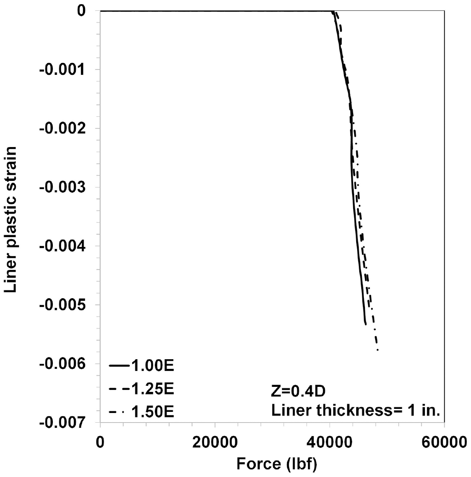
The maximum plastic strain for the liner against the applied force.

Figure 18 depicts the circumferential thrust and bending moment distribution around the CMP for a better understanding of the liner elastic modulus on the performance of the buried pipe and to support the idea that the pipe elastic modulus is more dominant. At the end of the analysis, the thrust and bending moment values are literally equal in all three situations, according to the results.

Figure 18.

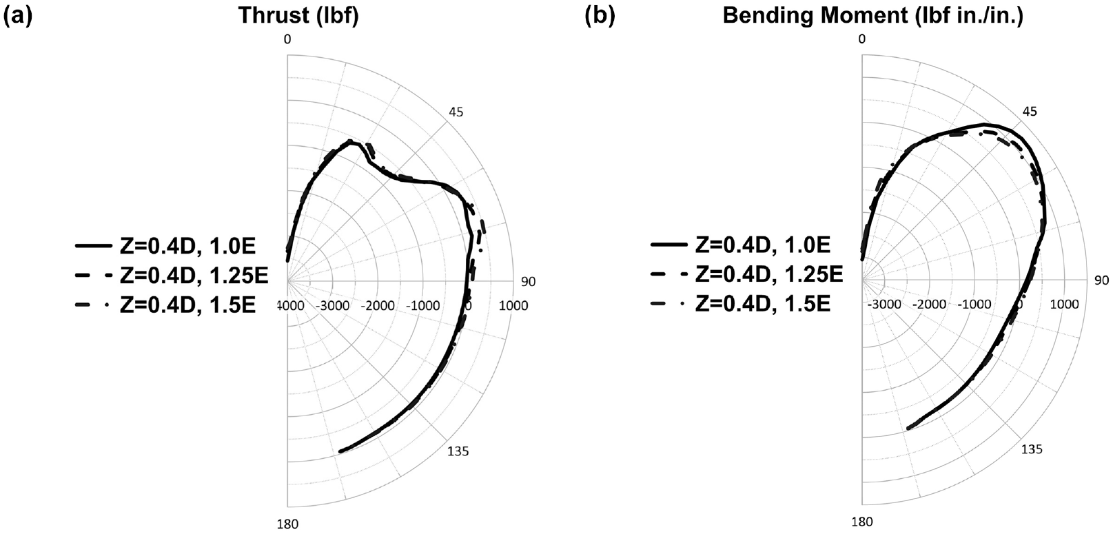
Effect of liner modulus on the simulated corrugated metal pipe (CMP) (liner thickness = 1 in. and 10 in. surface displacement): (a) circumferential thrust and (b) bending moment distribution.

Liner Thickness

In this section, four different liner thicknesses have been analyzed to see the performance of the liner thickness. Figure 19 shows the amount of peripheral deformation of the pipe in all different thicknesses. As it is known, when increasing the thickness of the liner layer from 0.25 in. to 1.5 in., the maximum vertical deformation of the pipe in the crown decreases from 8.7 in. to 2.9 in. (67% decrease). This value of decrease is meaningful in the region between the crown and the shoulder, which has the biggest role in tolerating the exerted load ( 31 ).

Figure 19.

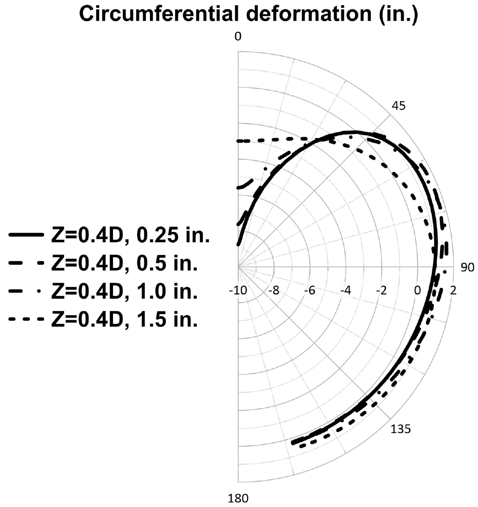
The quantity of circumferential deformations of the pipes in different situations at the end of analysis.

The moment of inertia is one of the critical factors that can influence the behavior of buried pipes. The performance of a hollow pipe is proportional to its moment of inertia. The moment of inertia of a corrugated plate is given by El-Atrouzy ( 32 ):

I = C_{1} b d^{2} t

(5)

where:

b = width of the corrugated sheet, in.

d = depth of corrugation, in.

t = thickness of the sheet (gauge), in.

C ₁ = $\frac{2}{15} \times$ [1+ $\frac{8}{3} \times (\frac{d}{e})$ ²], constant

e = pitch of corrugation (distance from ridge to ridge), in.

In this regard, increasing the liner thickness reduces the maximum internal diameter while increasing the moment of inertia. Figure 20 also depicts the maximum horizontal springline displacement and the maximum pipe crown displacement along the length of buried pipes. The results show that the thickest liner has experienced the least deformation along its length. For example, the maximum deformation between the center and tips of the pipe in the 1.5 in. liner and crown region is about 0.1 in., whereas this value is about 1.83 in. (1730% increase) in the 0.25 in. liner. In this regard, the thicker the liner, the better the response from the sprayed pipes will be. Figure 20b shows that the maximum horizontal settlement for 0.25 in. liner is less than that of 0.5 and 1.0 in. liner. The reason for this phenomenon is that the maximum vertical deflection at the crown for 0.25 in. liner is greater than in other situations; in this situation, more compactions might have occurred around the pipe, causing the pipe’s surrounding soil to be more solidified and compacted, resulting in a decrease in horizontal deflection. Also, it should be noted that the maximum horizontal displacement differences between the mentioned situations are less than 0.7 in., whereas this value is about 4 in. in the crown displacement.

Figure 20.

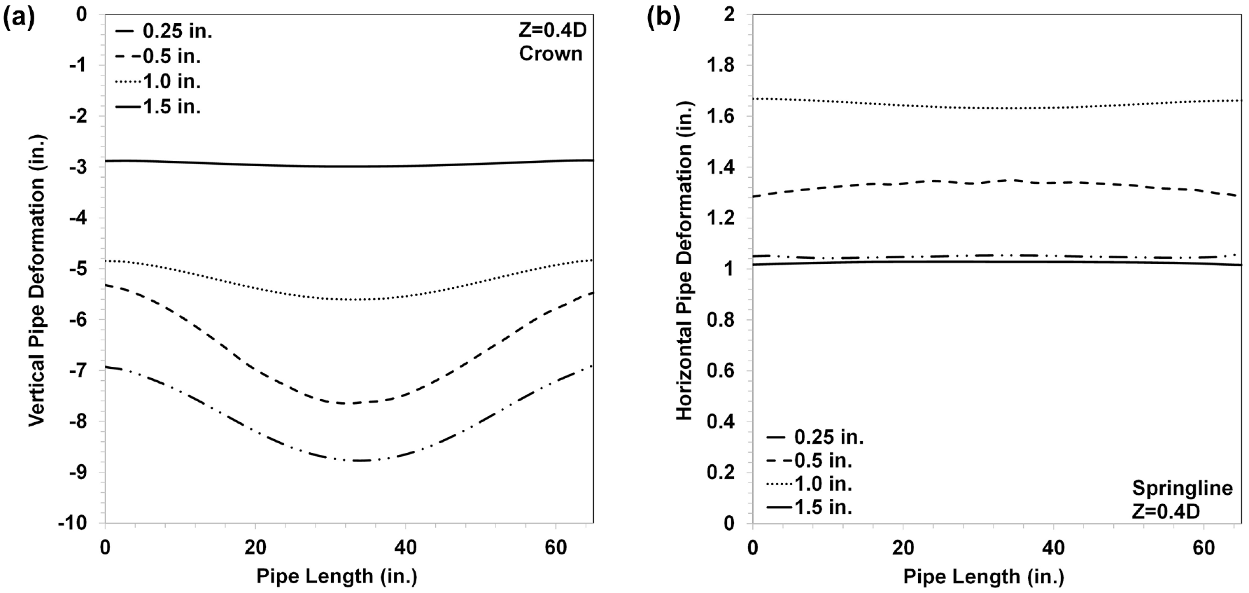
Deflections along the length of buried pipes: (a) the maximum pipe crown displacement and (b) the maximum pipe springline displacement at the end of analysis.

Figure 21 depicts the circumferential thrust and bending moment distribution around the CMP at the end of the analysis (10 in. surface displacement) to aid comprehension. The bending moment value is proportional to the moment of inertia, and as we discussed in the previous section, increasing the liner thickness increases the moment of inertia. In this regard, increasing the liner thickness from 0.5 in. to 1.5 in. reduced the maximum bending moment at the pipe crown from −5,467.69 lbf in./in. to −668.32 lbf in./in. (~87 reduction). As mentioned before, the results show the most susceptible region is the area between the crown and shoulder ( 30 ) in a way that the liner thickness doesn’t have any impact on the invert and haunch region of the pipes. Concerning the thrust values, the results show that the type of deformation can affect the force and bending moment in the pipe’s cross-section area. Because the 0.25 in. liner has more deformation in the crown and shoulder, the cross-section forces at the crest and valley may cancel out. In this case, the 0.25 in. liner has a lower thrust value in the crown region; however, in general, and in line with previous statements, the thickest liner (1.5 in.) provides the best overall performance.

Figure 21.

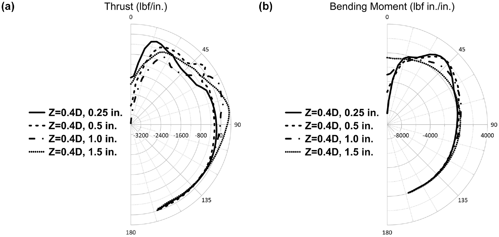
Simulated corrugated metal pipe (CMP) results at the end step of the model analysis: (a) circumferential thrust and (b) bending moment.

Concerning having a better perspective, we compared the liner’s first plastic strain point, crack starting point, and pipe starting plastic point as comparison points to gain a better understanding of which situations have better performance. Table 5 displays the stress values for the first plastic strain appearance for the liner and pipe over the loading surface for various scenarios, and it is clear that a higher embedment depth has the best performance in which the liner would be completely safe until the end of analyses (10 in. surface settlement), and the level of stress for the pipe to reach the plastic strain value was higher than in other situations. As previously stated, because the pipe has less strength than the liner, the pipe behavior takes precedence over the liner behavior, and by increasing the liner elastic modulus by 50%, the corresponding surface loading stress for the appearance of the plastic strain in the liner is literally fixed. To demonstrate the significance of embedment depth (Table 5), the results showed that increasing the embedment depth from 0.4D to 1.0D increased the corresponding surface loading stress by 382%.

Table 5.

The Surface Loading Stress Values for the First Plastic Strain Appearance for the Liner and Pipe

Parameters	Variables	Liner plastic strain appearance	Pipe plastic strain appearance
Liner thickness = 1.0 in. Liner elastic modulus (E) = 166e6 psf	Embedment depth = 0.4D	46.2 psf	17 psf
	Embedment depth = 0.7D	Remained elastic	45 psf
	Embedment depth = 1.0D	Remained elastic	82 psf
Liner thickness = 1.0 in. Embedment depth (Z) = 0.4D	E	46.2 psf	17 psf
	1.25 times of E	46.04 psf	16 psf
	1.5 times of E	45 psf	19 psf
Liner elastic modulus (E) = fixed Embedment depth (Z) = 0.4D	Liner thickness = 0.25 in.	28 psf	8 psf
	Liner thickness = 0.5 in.	31 psf	10 psf
	Liner thickness = 1.0 in	Remained elastic	82 psf
	Liner thickness = 1.5 in	Remained elastic	82 psf

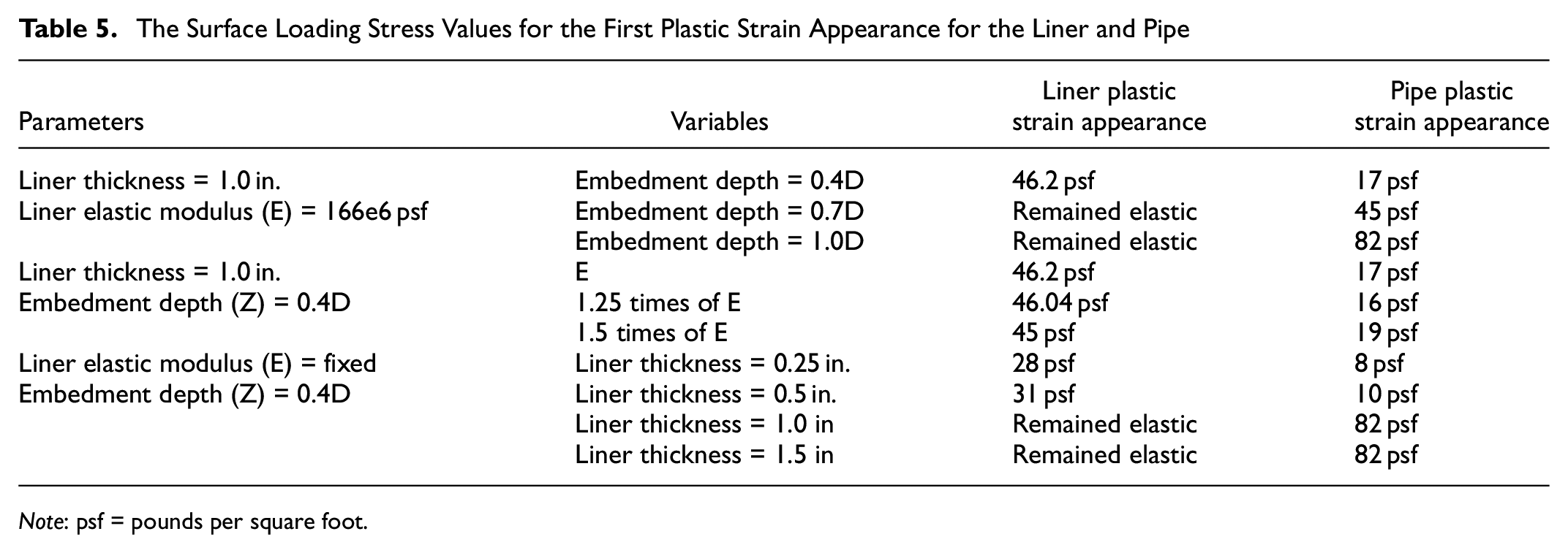
Note: psf = pounds per square foot.

Summary and Conclusions

The critical issue of corrosion and deterioration in CMPs and the critical need for their rehabilitation to maintain structural integrity were investigated in this paper. SAPLs as a quick and effective way to revitalize deteriorated CMPs have not been investigated through comprehensive experimental tests and FE studies. To bridge this gap, this research focuses on the calibration of a 3D full-scale FE model using data derived from thorough testing at the UTA CUIRE laboratory. These tests focused on circular invert cut CMPs that had been rehabilitated with polymeric SAPLs with liner thicknesses of 0.25, 0.5, and 1 in. To simulate the deterioration process, an 18-in. invert was removed from an intact CMP.

The paper in detail built a comprehensive 3D corrugated model in ABAQUS that accurately showed the test setup, allowing us to perform the calibration process. It effectively validated the capability of our FE model by meticulously comparing key parameters through the material parameters modified through the calibration process. This validated model was then used to generate some results for different scenarios.

The assumption of the first plastic strain as the first crack predicts the crack and the crack pattern in the CMP well.

From both the test and FEM results, it is seen that the rigidity of the pipe is increased with the increase in the thickness of the liner.

The drop in the load after the ultimate load is not predicted by the FE analysis, as the FEM model was a static general solver and was not modeled for the -post-failure analysis of the liner.

When it comes to pipe embedment depth, the results show that increasing the burial depth of the pipe from 0.4D (D: pipe diameter) to 0.7D reduces the maximum deformation of the pipe by approximately 31%. When the pipe’s burial depth was increased to 1.0D, this value increased to 58.9%.

Increasing the elastic modulus of the liner layer by 50% reduces the maximum amount of vertical deformation of the pipe between the center and side by about 30%. This value is approximately 35% in the pipe’s springline area.

By increasing the liner thickness from 0.25 in. to 1.5 in., the maximum bending moment at the pipe crown was reduced by approximately 87%. The results also show that the area between the crown and the shoulder is the most vulnerable.

The surface loading stress associated with the initial occurrence of plastic strain in the pipe body increased by 382% with an increase in the embedment depth of the rehabilitated pipes from 0.4D to 1.0D.

Limitations of the FE Model

The FE model was a static general solver and thus could not predict the load drop after the ultimate load.

Since the brittle polymeric material of the liner was modeled using the simple elastic–plastic model instead of crack models, a drop in load at the first crack was not observed in the FE model.

Footnotes

Acknowledgements

The authors would like to thank Ohio DOT (project leader), DelDOT, FDOT, MnDOT, NCDOT, NYSDOT, and PennDOT for supporting and participating in this research. Partner companies and consultants were LEO Consulting, LLC, Rehabilitation Resource Solutions, and American Structure Point, Inc. In addition, many thanks to Sprayroq, Contech Engineering, Forterra Pipe and Precast, HVJ Associates, MTS Systems Corporation, and Micro-Measurement for providing various products and services that were essential for the soil box tests. The authors also thanks the University of Texas at Arlington’s CUIRE laboratory for their invaluable assistance and support in carrying out the soil box tests that were carried out during this study.

Author Contributions

The authors confirm contribution to the paper as follows: study conception and design: S. Raut, M. Azizian, X. Yu, A. D. Tehrani, H. Chimauriya; data collection: S. Raut, M. Azizian, A. D. Tehrani, H. Chimauriya; analysis and interpretation of results: S. Raut, M. Azizian, X. Yu; draft manuscript preparation: S. Raut, M. Azizian, X. Yu, H. Chimauriya. All authors reviewed the results and approved the final version of the manuscript.

Declaration of Conflicting Interests

The authors declared no potential conflicts of interest with respect to the research, authorship, and/or publication of this article.

Funding

The authors disclosed receipt of the following financial support for the research, authorship, and/or publication of this article: This research is part of the NCHRP project 31347 (2017), which is part of the National Cooperative Highway Research Program (NCHRP). NCHRP is administered by the Transportation Research Board (TRB) and funded by participating member states of the American Association of State Highway and Transportation Officials (AASHTO). NCHRP also receives critical technical support from the Federal Highway Administration (FHWA), United States Department of Transportation.

ORCID iDs

Samrat Raut

Hiramani Raj Chimauriya

Amin Darabnoush Tehrani

Mohammad Najafi

Xinbao Yu

Data Accessibility Statement

In the spirit of open and collaborative research, we are pleased to announce that all the data and materials used in this study are readily available for sharing with fellow researchers and interested parties.

References

Najafi

Pipeline Infrastructure Renewal and Asset Management. McGraw Hill Professional, New York, NY, 2016.

Najafi

Trenchless Technology: Planning, Equipment, and Methods. McGraw Hill Professional, Chicago, IL, 2013.

Garcia

D. B.

Moore

I. D.

Performance of Deteriorated Corrugated Steel Culverts Rehabilitated with Sprayed on Cementitious Liners Subjected to Surface Loads. Tunneling and Underground Space Technology, Vol. 47, 2015, pp. 222–232.

Masada

Structural Benefit of the Concrete Paving of Steel Culverts Inverts. Ohio Department of Transportation, Columbus, 2017.

Campbell

Three-Dimensional Finite Element Modelling of the Corroded Corrugated Metal Pipe Culverts. Thesis. Dalhousie University, Halifax, Canada, 2018.

Chimauriya

H. R.

Laboratory Test and Finite Element Modeling of the Invert Removed Corrugated Steel Culvert Buried Under the Shallow Cover. University of Texas at Arlington, 2019.

CUIRE. Structural Design Methodology for Spray Applied Pipe Liners in Gravity Storm Water Conveyance Conduits-3rd Quarterly Progress Report. Ohio Department of Transportation, Columbus, 2018.

Raut

Experimental and 3D Finite Element Analyses of Invert-Removed Circular Corrugated Metal Pipe Culverts Renewed with Polymer Spray-Applied Pipe Lining. University of Texas at Arlington, 2020.

El-Sawy

K. M.

Three-Dimensional Modeling of Soil-Steel Culverts Under the Effect of Truckloads. Thin-Walled Structures, Vol. 48, No. 8, 2003, pp. 747–768.

10.

Taher

M. E.

Moore

I. D.

Effect of Wall Corrosion and Backfill Erosion on the Strength of Deteriorated Metal Culverts. International Society for Trenchless Technology, Berlin, Germany, 2011.

11.

Elshimi

T. M.

Three-Dimensional Non-Linear Analysis of Deep Corrugated Steel Culverts. Thesis. Queen’s University, Kingston, Canada, 2011.

12.

Mai

V. T.

Hoult

N. A.

Moore

I. D.

Effect of Deterioration on the Performance of the Corrugated Steel Culverts. Journal of Geotechnical and Geoenvironmental Engineering, Vol. 140, 2013, pp. 1–11.

13.

Smith

Hoult

N. A.

Moore

I. D.

Role of Grout Strength and Liners on the Performance of Slip-Lined Pipes. Journal of Pipeline Systems Engineering and Practice, Vol. 6, No. 4, 2015, p. 04015007.

14.

Ezzeldin

El Naggar

Three-Dimensional Finite Element Modeling of Corrugated Metal Pipes. Transportation Geotechnics, Vol. 27, 2021, p. 100467.

15.

Kunecki

Kubica

Full-Scale Laboratory Tests and FEM Analysis of Corrugated Steel Culverts Under Standardized Railway Load. Archives of Civil and Mechanical Engineering, Vol. 4, No, 4, 2004, pp. 41–53.

16.

Kang

J. S.

Han

T. H.

Kang

Y. J.

Yoo

C. H.

Short-Term and Long-Term Behaviors of Buried Corrugated High-Density Polyethylene (HDPE) Pipes. Composites Part B: Engineering, Vol. 40, No. 5, 2009, pp. 404–412.

17.

American Association of State Highway and Transportation Officials. Standard Specifications for Highway Bridges. AASHTO, Washington, D.C., 2002.

18.

ASTM D2321. Standard Practice for Underground Installation of Thermoplastic Pipe for Sewers and Other Gravity-Flow Applications. ASTM International, West Conshohocken, PA, 2008.

19.

British Standard Institute (BSI). Thermoplastics Ancillary Fittings of Nominal Sizes 110 and 160 for Below Ground Gravity Drainage and Sewerage. BS 4660. BSI, London, 2000.

20.

ASTM Standard A929M. Standard Specification for Steel Sheet, Metallic-Coated by the Hot-Dip Process for Corrugated Steel Pipe. ASTM International, West Conshohocken, PA, 2017.

21.

ASTM Standard D2487-17. Standard Practice for Classifications of Soils for Engineering Purposes (Unified Soil Classification System). ASTM International, West Conshohocken, PA, 2011.

22.

ASTM Standard D698-12. Standard Test Methods for Laboratory Compaction Characteristics of Soil Using Standard Effort. ASTM International, West Conshohocken, PA, 2011.

23.

Paredes

Evaluation of Spraywall Structural Coating. NTPEP, Austin, TX, 2018.

24.

Darabnoush Tehrani

Kouchesfehani Kohankar

Chimauriya Raj

Raut

Najafi

Structural Evaluation of the Invert -Cut Circular and Arch Shape Corrugated Steel Pipes through Laboratory Testing. Canadian Journal of Civil Engineering, Vol. 48, 2020, pp. 187–201.

25.

Azizian

Moghaddas Tafreshi

S. N.

Darabi

N. J.

Experimental Evaluation of an Expanded Polystyrene (EPS) Block-Geogrid System to Protect Buried Pipes. Soil Dynamics and Earthquake Engineering, Vol. 129, 2020, p. 105965.

26.

Moghaddas Tafreshi

S. N.

Joz Darabi

Dawson

A. R.

Azizian

Experimental Evaluation of Geocell and EPS Geofoam as Means of Protecting Pipes at the Bottom of Repeatedly Loaded Trenches. International Journal of Geomechanics, Vol. 20, No. 4, 2020, p. 04020023.

27.

ABAQUS/CAE User’s Guide, Abaqus 6.14, SIMULIA. 2014. http://130.149.89.49:2080/v2016/index.html.

28.

Elshimi

T. M.

Moore

I. D.

Modeling the Effects of Backfilling and Soil Compaction Beside Shallow Buried Pipes. Journal of Pipeline Systems Engineering and Practice, Vol. 4, No. 4, 2013, pp. 1–7.

29.

Khalaj

Azizian

Moghaddas Tafreshi

S. N.

Mašek

Laboratory Investigation of Buried Pipes Using Geogrid and EPS Geofoam Block. IOP Conference Series: Earth and Environmental Science, Vol. 95, No. 2, 2017, p. 022002.

30.

Nakhostin

Kenny

Sivathayalan

Numerical Performance Assessment of Buried Corrugated Metal Culvert Subject to Service Load Conditions. Canadian Journal of Civil Engineering, Vol. 48, No. 2, 2020, pp. 99–114.

31.

Chaallal

Arockiasamy

Godat

Field Test Performance of Buried Flexible Pipes Under Live Truck Loads. Journal of Performance of Constructed Facilities, Vol. 29, No. 5, 2015, p. 04014124.

32.

El-Atrouzy

M. N.

Structural Properties of Corrugated Sheets Used in Cylindrical Shells. Thesis. University of Windsor, Canada, 1969.

Three-Dimensional Finite Element Modeling of Spray-Applied Pipe Liners Repaired Corrugated Metal Pipes Buried Under Shallow Cover

Abstract

Keywords

Soil Box Test of Lined Circular Invert-Cut CMPs in a Soil Box

Geometry of The Soil Box

CMP Pipe

Soil and Burial Configuration

Polymer SAPL

Instrumentation

Loading Configuration

Finite Element Model

Model Setup

Material Model

Soil Properties

CMP and Liner Properties

Mesh Sensitivity

Soil–Pipe and Pipe–Liner Interactions

Model Step

Results and Discussion

Model Verification

Verification of Load Displacement

Verification of Pressure and Displacement

Verification of Strains

Parametric Study

Burial Depth

Elastic Modulus of the Liner Layer

Liner Thickness

Summary and Conclusions

Limitations of the FE Model

Footnotes

Acknowledgements

Author Contributions

Declaration of Conflicting Interests

Funding

ORCID iDs

Data Accessibility Statement

References