Sage Journals: Discover world-class research

Abstract

Safe railway operation is vital for public safety, the environment, and property. Concurrent with climbing amounts of rail traffic on the Canadian rail network are increases in the last decade in the annual crash counts for derailment, collision, and highway railroad grade crossings (HRGCs). HRGCs are important spatial areas of the rail network, and the development of community areas near railway tracks increases the risk of HRGC crashes between highway vehicles and moving trains, resulting in consequences varying from property damage to injuries and fatalities. This research aims to identify major factors that cause HRGC crashes and affect the severity of associated casualties. Using these causal factors and ensemble algorithms, machine learning models were developed to analyze HRGC crashes and the severity of associated casualties between 2001 and 2022 in Canada. Furthermore, spatial autocorrelation and optimized hotspot analysis tools from ArcGIS software were used to identify hotspot locations of HRGC crashes. The optimized hotspot analysis shows the clustering of HRGC crashes around major Canadian cities. The analysis of cluster characteristics supports the results obtained for causal factors of HRGC crashes. These research outcomes help one to better understand the major causal factors and hotspot locations of HRGC crashes and assist authorities in implementing countermeasures to improve the safety of HRGCs across the rail network.

Keywords

artificial intelligence and advanced computing applications data analytics machine learning passenger rail transportation safety performance and analysis crash analysis

The railway industry of Canada is a major contributor to the country’s economy. The safety of the rail network is crucial, as crashes on the railway network can seriously harm the system environment and result in numerous fatalities ( 1 , 2 ). Canada’s rail network is the third largest in the world, with more than 41,700 km of rail tracks featuring 25,155 highway railroad grade crossings (HRGCs) ( 3 , 4 ). A HRGC is an intersection of railway tracks and roads at the same grade level ( 4 ). Crashes at HRGCs are a safety concern and have attracted the attention of transport authorities, the public, and the railway sector ( 5 ). The expansion of municipalities and the development of high-population areas near railway lines pose a greater risk of crashes that can result in fatalities, injuries, extensive property damage, and delays in railway and highway traffic, making HRGCs spatial areas paramount for transportation safety ( 2 , 6 , 7 ). Between 2011 and 2020, 10,705 railway crashes were recorded in Canada, with the leading categories being non-main-track derailments (49.3%), followed by HRGC crashes (15.4%) (Table 1) ( 8 ). A non-main-track derailment is when one or more railcar wheels come off the rail surface on non-main tracks (such as yard rail lines). These crashes usually happen at speeds below 10 mph and are considered low-consequence crashes ( 8 ). On the other hand, crashes at HRGCs that include trains and highway vehicles are known as HRGC crashes ( 9 ). These crashes usually happen at track speed between vehicles and a moving train and are considered high-consequence. According to the data in Table 1, the number of HRGC crashes (1648) is less than the number of non-main-track derailment crashes (5278), but the fatality counts for HRGC crashes is far higher (227 versus 1). Thus, HRGC crashes are considered higher risk than non-main-track derailments and can result in more fatalities ( 10 ).

Table 1.

Rail Crashes Based on Crash Type (2011–2020) ( 8 )

Type of crash	Crash count	Percentage	Fatality count
Non-main-track derailments	5278	49.30	1
Highway railroad grade crossing crashes	1648	15.40	227
Other (e.g., fire, employee/passenger crashes)	1346	12.60	20
Non-main-track collisions	933	8.71	3
Main-track derailments	825	7.70	54
Trespasser crashes	625	5.83	403
Main-track collisions	50	0.47	0
Total	10,705	100	708

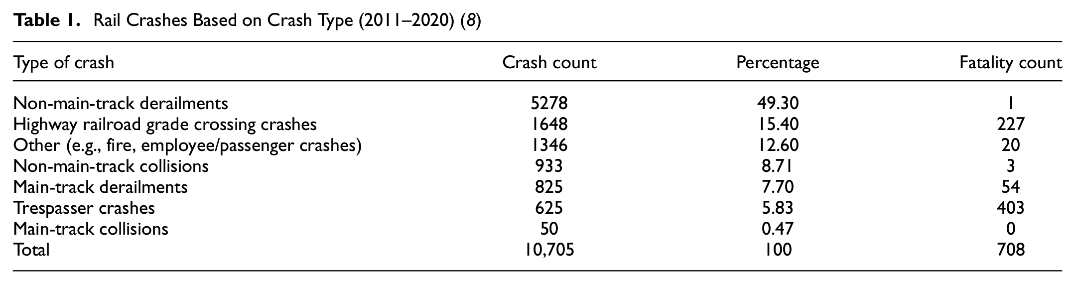
Figure 1 shows the time-trend analysis of HRGC crashes and associated casualties in Canada from 2011 to 2020. The analysis used crash and casualty counts from the Transportation Safety Board of Canada (TSB) dataset. These counts were normalized for comparison using million train miles (MTM) data for each year. HRGC crash counts per MTM have not changed much over the last decade (Figure 1a); however, fatality and serious injury counts per MTM have fluctuated. Fatality and serious injury percentages for HRGC crashes have shown an overall decreasing trend in the last decade; yet, the percentage of fatalities (Figure 1b) and serious injuries (Figure 1c) caused by HRGC crashes is high, at ~30% in 2020. HRGC crashes were the second-highest contributor to railway fatalities after trespasser crashes from 2011 to 2020; however, HRGC crashes have been the highest contributor to serious injuries on the Canadian railway in the last decade ( 8 ).

Figure 1.

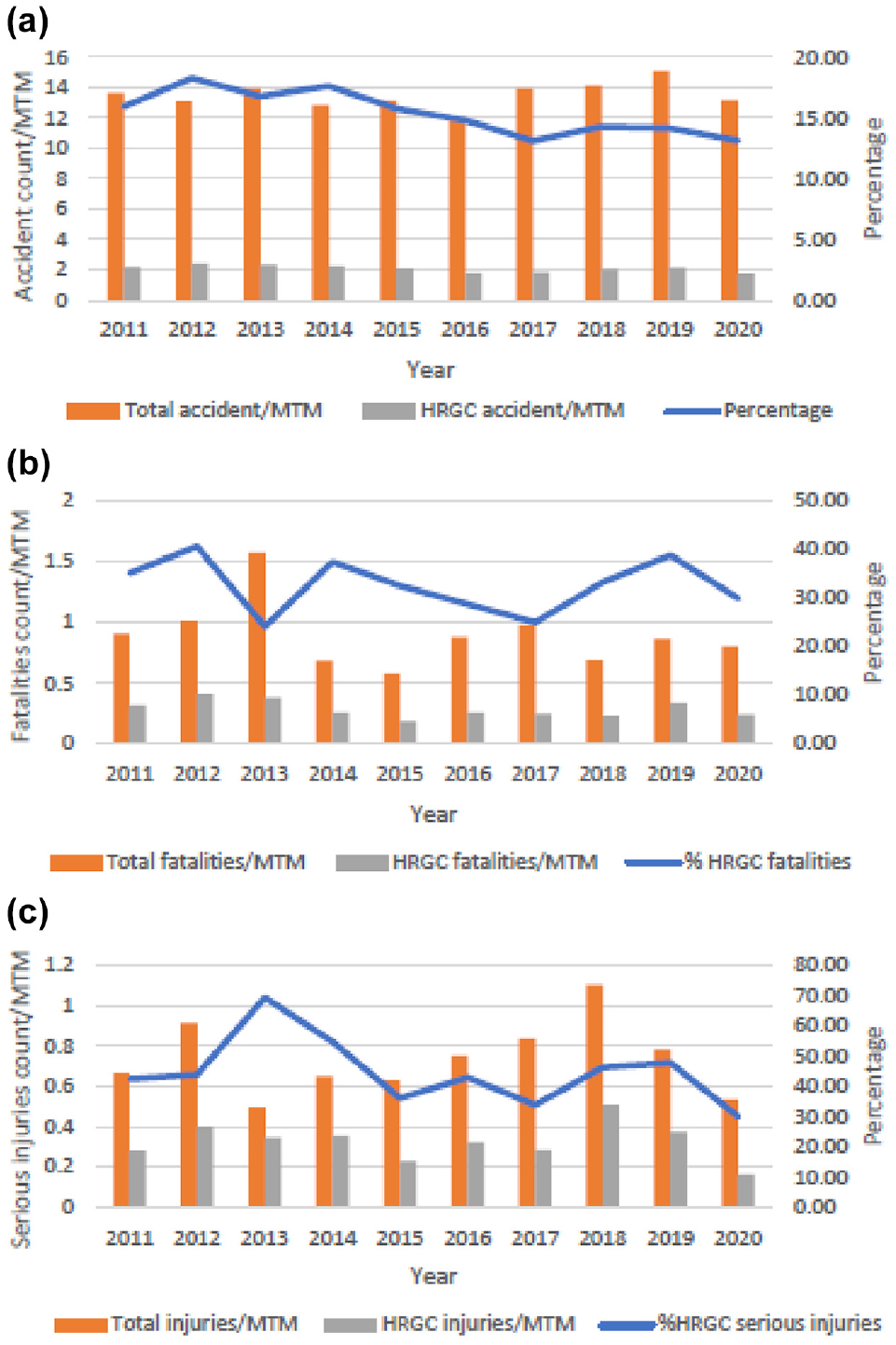
Trends in (a) highway railroad grade crossing (HRGC) crashes, (b) fatalities, and (c) serious injuries (2011–2020) ( 8 ).

Figure 1b shows a sudden drop in 2013 concerning %HRGC fatalities. In 2013, 47 fatalities were reported in the “main-track derailment” category because of a crash in Lac-Mégantic, Quebec, which resulted in a lower % of HRGC fatalities. Thus, the %HRGC fatalities value is considered an outlier for fatality data 2013. Figure 1c shows that the %HRGC serious injuries experienced a sudden rise in 2013. The total serious injury count was 39 in 2013, and fewer injuries were reported in other categories. This resulted in an unusually large contribution of HRGC crashes to the total. Thus, the 2013 value is considered an outlier for serious injury data ( 8 ).

High occurrences and consequences of HRGC crashes have raised concern, resulting in many studies aimed at improving the safety of HRGCs. For instance, a study by Lu et al. ( 11 ) uses generalized linear models, such as the Poisson, Bernoulli, and hurdle Poisson models, to predict HRGC crash frequency. The dataset contained crossing, highway, and rail traffic variables of HRGC crashes in North Dakota, U.S.A., between 1996 and 2014. The study highlights variables such as average daily vehicle traffic, daily train traffic, warning system, nighttime through-train traffic, train maximum speed, and the number of traffic lanes on the highway as contributors to HRGC crashes. Moke and Savage ( 12 ) use negative binomial regression on HRGC crash data from the U.S.A. from 1975 to 2001. Two separate models are developed in their study, one for predicting the number of HRGC crashes and another for predicting the number of casualties that occurred in HRGC crashes. The results indicate that daily train and vehicle traffic increases the risk of HRGC crashes and fatality counts, while an active warning system, locomotives with ditch lights, and safety campaigns reduce the risk. Another study by Brod and Gillen ( 13 ) developed two models for HRGC risk assessment. The authors use the zero-inflated negative binomial model to predict HRGC crashes and the multinomial regression model to find the severity probability (fatal, injury, and no injury). The study shows significant relations among HRGC characteristics, warning devices, and traffic exposure in HRGC crashes. Brabb et al. ( 14 ) studied HRGC crash data to analyze various factors in injuries and fatalities caused by HRGC crashes. The report identifies the effects of traffic, driver demography, environment, and crossing characteristics on the severity of casualties in HRGC crashes. Soleimani et al. ( 15 ) use Federal Railroad Administration (FRA) data to develop a HRGC consolidation model for public crossings using text mining, spatial analysis, and an extreme gradient boosting (XGBoost) algorithm to identify possible HRGCs that can be considered for closure in the future.

Several recent studies employ machine learning (ML) models to improve the safety of HRGCs. For instance, Zheng et al. ( 16 ) used ML to identify HRGC crashes based on crash risk in the U.S.A. between 1996 and 2014. The classification model was developed using a decision tree (DT) and gradient-boosting (GB) algorithm and obtained good classification accuracies (0.7705) for crashes and no crash cases at HRGCs. The authors found factors such as daytime train movement, nighttime train movement, daily train traffic, train speed, and highway speed are the most important factors related to HRGC crashes. Another study by Lasisi et al. ( 17 ) uses various ML classifiers, such as the support vector machine (SVM), random forest (RF), Gaussian naïve Bayes (GNB), multi-layer perceptron-neural network (MLP-NN), and logistic regression (LR), to predict casualties resulting from HRGC crashes using HRGC casualty data from California, U.S.A. High prediction accuracy (0.989) is achieved with the SVM. A total of 15 features are considered, including features related to railway and highway traffic and crossing characteristics that revealed train speed, average daily train, and vehicle traffic are essential factors affecting casualties in HRGC crashes.

The spatial distribution and hotspot locations of HRGC crashes have been assessed using spatial autocorrelation and optimized hotspot analysis using ArcGIS software. These tools generate significant and valuable spatial analysis results by employing crash counts/rates and geographic data as inputs. The results of spatial autocorrelations and optimized hotspot analysis show the statistically significant locations on maps called hotspot locations of crashes. Various studies have been conducted to analyze aviation crashes and road crashes using different ArcGIS software. Li and Liang ( 18 ) studied aviation crashes in Florida, U.S.A., using hotspot analysis tools and data from the National Transportation Safety Board (NTSB) from 2002 to 2017 and reported 75 hotspot locations for aviation crashes. Prasannakumar et al. ( 19 ) studied spatial clustering of road crashes in India and Mulugeta Tola and Gebissa ( 20 ) in Ethiopia using ArcGIS. The results of these studies give information on hotspot and coldspot locations, which provide insights for traffic management and crash reduction.

To the authors’ knowledge, limited research has been conducted on HRGC crashes in Canada’s rail network. Many contributing factors are involved in HRGC crashes, including highway and railway factors. The study by Heydari and Fu ( 21 ) uses Canadian railway HRGC data (2008–2013) to assess the effects of HRGC location attributes. The study only investigates a few factors, such as train speed, road speed, daily train traffic, daily vehicle traffic, and the number of highway lanes. Furthermore, a study by researchers at the University of Waterloo developed a tool called GradeX to assess HRGCs in Canada ( 4 ). It supports decision-making so authorities can identify high-risk HRGCs. The tool uses factors such as daily traffic of trains and vehicles, speed of trains and vehicles, location, and warning system at HRGCs. However, in both studies, important factors such as visibility, season, type of vehicle, and driver actions were not included. To address this research gap, all of these variables were considered in this research. This study focuses on identifying the most significant causal factors for HRGC crashes and the severity of casualties and helps minimize the chances and consequences of HRGC crashes. These causal factors are used with ensemble classifiers to analyze HRGC crashes based on crash risk and severity of associated casualties. The results can inform the implementation of strategies to increase HRGC safety in Canada. However, targeting all HRGCs within a rail network concerning the implementation of safety strategies is a very wide-scope and highly capital-intensive task. Thus, locating the hotspots of HRGC crash locations is beneficial in allocating appropriate resources. ArcGIS software helps not only visualize the spatial distribution of HRGC crash locations but also locate hotspot locations. Information about hotspot locations and causes of HRGC crashes will contribute to quicker implementation of safety strategies and enhanced safety at HRGCs.

The main objectives of this research are as follows:

identify the causal factors of HRGC crashes and the severity of associated casualties using a feature selection technique (ExtraTree classifier);

apply ensemble-supervised ML algorithms (RF, AdaBoost, and XGBoost) to analyze HRGC crashes;

apply ensemble-supervised ML algorithms (RF, AdaBoost, and XGBoost) to analyze casualty severity in HRGC crashes; and

determine HRGC crash hotspot locations using ArcGIS software for Canada’s rail network.

Methods

Data for the ML Model

The HRGC crossing information and crash data were taken from two public sources. The HRGC inventory data, which was collected from the Government of Canada website ( 4 ), was used in the analysis of HRGC crashes. The dataset contained information about HRGC crashes at every HRGC in the Canadian rail network. The original HRGC inventory dataset ( 4 ) contained 25,155 samples with 26 feature columns, such as the number of daily vehicles, number of daily trains, maximum road speed, maximum train speed, type of protection, and number of tracks at the HRGC.

The data containing information about the severity of casualties associated with HRGC crashes were taken from the TSB’s Railway Occurrences Database System (RODS) ( 22 ) and were used in the severity of casualty analysis using the ML model. The dataset included information about casualties reported in HRGC crashes. The original dataset contained information on 6581 HRGC crashes with 348 features, such as rank, HRGC-ID, railway owner, region, province, and number of daily vehicles. Figure 2 shows the methodology for this research.

Figure. 2.

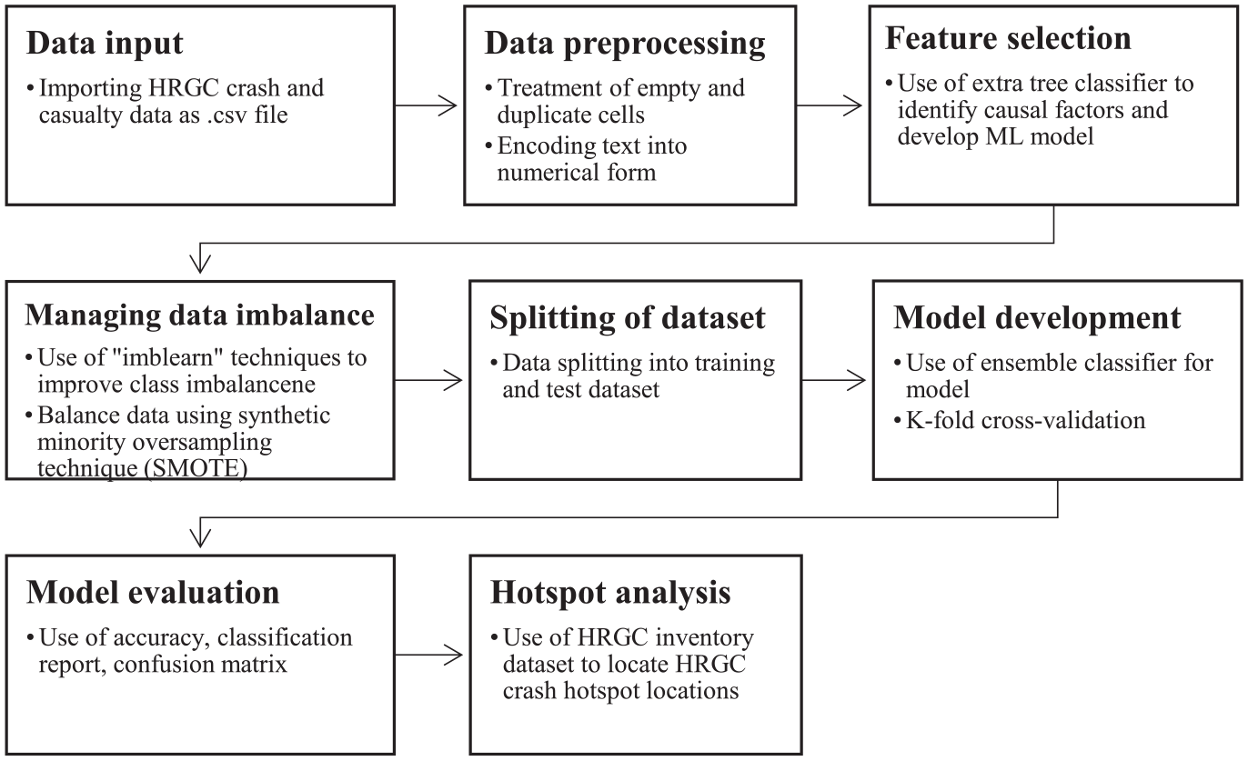
Methodology for the supervised classification machine learning (ML) model.

Data Preprocessing

The raw datasets from the data sources need preprocessing to address missing cell entries, duplicate rows, and categorical variables ( 23 , 24 ). If not treated beforehand, these missing cell entries and duplicate rows in datasets cause biased performance estimation for the ML model. Techniques such as deleting rows with missing cells or entering arbitrary or mean values of the feature are commonly used to manage missing cell entries ( 25 ). The datasets used in the present study contain many feature columns, including location, highway, railway, and environmental factors. However, some of the feature columns in the dataset had empty cells and therefore were excluded. In addition, duplicate row entries and feature columns with less important information were manually removed from the datasets.

The HRGC inventory dataset contained feature columns such as rank, Transport Canada (TC) number, railway owner, region, and province; these were removed because they added little value to the analysis (n = 15). Some sample entries were removed afterward as they had empty cell entries (n = 6001). Categorical features such as “Access,”“Protection,”“Regulator,” and “IsUrban” were converted to numeric variables using “LabelEncoder,” which generated the matrix of data for the classification. Finally, 10 input features and one output feature were selected, with 19,154 samples for feature selection. The output feature is a binary class feature, where 0 (zero) indicates a HRGC with no crash in history and 1 (one) indicates a HRGC with at least one crash reported in the history. Definitions of each feature of the model are given in Appendix A.

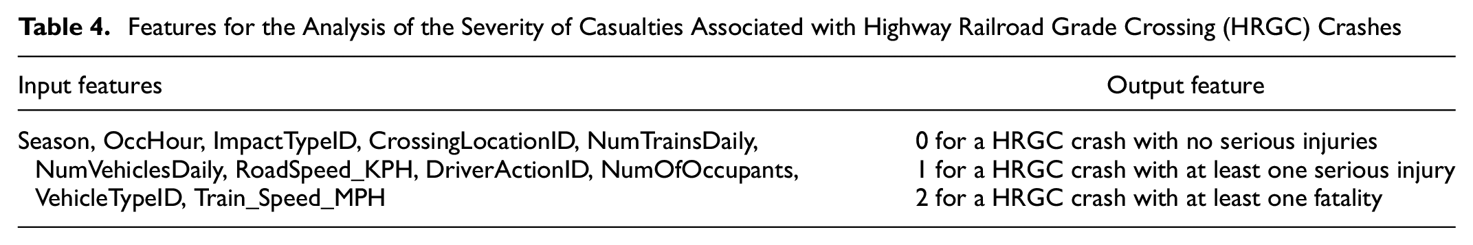
The HRGC casualty dataset from the RODS contained features such as railway owner, region, province, and subdivision that were not useful for the supervised classification model and, therefore, were removed from the dataset. In addition, some of the feature columns (such as dangerous goods released cars, ballast type, and temperature) were reported with many empty cell entries and therefore were also removed from the dataset (n = 330). Furthermore, duplicate sample entries were removed from the dataset (n = 174). Finally, after the data preprocessing, 17 input features and one output feature with 555 samples were selected. In addition, three more features were incorporated into the dataset to examine the effect of season, hour of the day, and train speed. The features named “Season” and “OccHour” were extracted using the time and date for given crashes from the dataset. The time was reported in “hhmm” format in the “OccTime” column. Thus, “OccHour” is extracted as “hh” from the “OccTime” column. “Season” is extracted from the “OccDate” feature column. The season of a crash was given a categorical variable, with 1 for winter (December to February), 2 for spring (March to May), 3 for summer (June to August), and 4 for fall (September to November). The “Train_Speed_MPH” feature was extracted using the HRGC-ID number for the effect of train speed on casualties associated with HRGC crashes. The HRGC inventory dataset was used to extract train speed values based on the HRGC-ID for the RODS dataset. The output feature is a multi-class feature, where 0 (zero) indicates a HRGC crash with no serious injury, 1 (one) indicates a HRGC crash with at least one serious injury, and 2 (two) indicates a HRGC crash with at least one fatality. The final classification dataset had 20 input features and one output feature with 555 samples. Definitions of features are given in Appendix B.

Feature Importance by the ExtraTrees Classifier

An ExtraTrees classifier is an ensemble method that helps identify the most important features for obtaining the classifier’s output ( 26 ). As a part of the ExtraTrees classifier, initial training samples are used to build each DT in the extra tree forest. Then, each tree is given a random sample of k features from the features at each test node. It must choose the best feature to divide the data according to a criterion (Gini index or entropy). The feature importance value ranges from zero to one, with higher feature importance values indicating features with a higher pertinence for predicting the output ( 27 ).

Based on the output of the ExtraTrees classifier, the optimum number of features is selected from the dataset for the classification model. According to the ranking of features in the ExtraTree classifier, an optimum number of features can be selected by assessing the accuracy value of the classification model for different numbers of features ( 28 ). When less than an optimum number of features is selected, the model gives a low accuracy value for the classification model. When the number of features increases, the accuracy value increases. However, the accuracy value will not significantly improve after the optimal number of features is reached. To determine the optimal number of features for developing the classification model of HRGC crashes and severity of casualty, a comparison of accuracy values was conducted using different feature subsets ranked by the results of the ExtraTree classifier. The goal was to identify the subset of features that achieved the highest accuracy in the classification model. This approach ensured the classification model was built using the most relevant and influential features, improving performance ( 29 ). The classification model takes a long time to train and test a dataset and can be computationally expensive when more than optimum features are selected ( 30 ).

Data Balancing

Initial analysis of the datasets showed an imbalance in class distribution (i.e., one class label has many observations, and the other has a small number of observations [ 24 ]). Imbalanced datasets cannot be used for conventional classification algorithms because such algorithms are based on three main assumptions: (i) the use of the precision of the model for assessment criteria; (ii) a nearly equal distribution of classes in the dataset; and (iii) the consequences of incorrect prediction of the class are identical for every class ( 31 ). These assumptions are not valid for most real-world datasets, which often have an imbalanced distribution of classes ( 32 ). High-performance classification models are built with a balanced dataset, which has near-equal sample counts for every class ( 33 ). To balance the class distribution, advanced techniques from the “imblearn” package in Python, such as the oversampling technique, undersampling technique, and synthetic minority oversampling technique (SMOTE), are available ( 34 ).

The oversampling technique increases the minority class samples by duplication and equalizes the class distribution but raises concerns about overfitting. On the other hand, the undersampling technique reduces the number of majority class samples, which leads to the omission of helpful information about a dataset ( 35 ). Another applicable technique is the introduction of synthetic samples around the existing samples, called the SMOTE, which creates minority samples by linear interpolating two identical classes using Equation 1 and adding them to the dataset ( 31 ):

X_{New} = X_{i} + rand (0, 1) \times (X_{i} - X_{j})

(1)

The SMOTE approach uses sample X_i of a given class from the dataset and calculates the distance from neighboring identical classes. The neighboring sample X_j will be randomly selected to populate new X_New using Equation 1. Therefore, the SMOTE can reduce overfitting and improve the classification model performance ( 31 ). Therefore, the SMOTE technique was used in our study. Data balancing is performed after the feature selection process because the SMOTE algorithm is applied to address a class imbalance in the dataset. Performing feature selection before data balancing ensures that the selected features are based on the original distribution of the data, which helps preserve the intrinsic information and relationships present in the original dataset and allows for more accurate and meaningful feature evaluation ( 36 ).

Splitting of the Dataset

For supervised ML, datasets are divided into training and testing datasets using the “test_train_split” method with stratified parameters. This method divides the dataset according to the input ratio from the user, and stratify parameter splits the dataset with an identical output class ratio in both the training and testing datasets. In this research, an 80:20 split ratio was used, meaning 80% of the data were partitioned into a training dataset and 20% into a testing dataset. In supervised ML, a training dataset is used to train the model, which allows the model to learn. After training, model performance is evaluated using the testing dataset ( 37 ).

Classification Model Development

Ensemble classification algorithms were used in research to implement ML models. An ensemble classifier method is a meta-approach for improving the predictive performance of the ML model ( 38 ). Ensemble classifiers generate one optimal ML model by combining multiple base models. The ensemble method is advantageous because it guarantees the prediction and provides a ML model with high stability and resilience. Vijaya and Sivasankar ( 39 ) compared ensemble and conventional classifiers to predict telecommunication customer churn. The outcome supported that the accuracy of ensemble classifiers, such as boosting and bagging, is greater than traditional classifiers. Therefore, this research utilizes several ensemble-supervised ML classification models, such as RF, AdaBoost, and XGBoost.

The RF classifier employs DTs as individual models and uses bagging as an ensemble method ( 40 ). Bagging is fitting several models to various samples of the same dataset and averaging the resulting predictions. The algorithm develops many trees, which happens in parallel, and then these trees vote for the most popular class ( 41 ). The algorithm has two phases: the first is the development of the RF, and the second is the prediction of results from the RF developed in earlier stages. As the RF uses the bagging method, it helps to reduce overall variance by combining the results of several classifiers trained on various training data samples. The RF classifier requires considerable computational power and time for training the model, as it creates several DTs to integrate their outputs. For the RF, the greater the number of trees, the better the result of the model. One fundamental problem that can worsen the results of the RF algorithm is overfitting. However, when the RF classifier has sufficient trees for the model, then the model’s outcome is not prone to overfitting ( 42 ). For the RF classifier, all the hyperparameters were selected with their default values.

The AdaBoost classifier employs DTs as individual models and uses boosting as an ensemble method. Boosting is the repetitive application of a weak learning algorithm to different distributions over the training data and then merging the weak learner’s classifiers into a single composite classifier. AdaBoost is a popular ensemble ML method that targets misclassified instances in a previous weak classifier while training a new weak classifier. Obtaining high accuracy in the classification model is a primary objective; however, achieving high accuracy with only one classifier may not be possible. This problem can be rectified when multiple weak classifiers are employed, as each one gradually learns from the misclassified samples of the previous classifier. When training a new weak classifier, the weights of training samples are changed to improve learning. The weights are increased (decreased) for training samples that are incorrectly (correctly) classified in weak classifiers ( 43 ). The AdaBoost algorithm is easy to implement, flexible, and prone to overfitting. However, it is sensitive to noisy data and outliers and takes longer to train as it trains the weak classifiers individually ( 44 ). For the AdaBoost Classifier, n_estimator = 500 was selected, and the rest of the hyperparameters were selected with their default values.

XGBoost is a supervised ensemble ML algorithm that uses the gradient-boosted DT as a model and boosting as an ensemble method. The input variables are assigned weight factors used by the gradient-boosted DT to predict the results. Variables that the previous weak learners incorrectly anticipated are given more weight before being placed into the following DT. The models trained with this approach provide a more accurate and potent model for ML applications ( 45 ). The model is popular because of its ability to manage sparse data and parallel and distributed computing while handling large samples ( 46 ). By incorporating regularization parameters, the learning rate, and column subsampling, XGBoost lessens overfitting and improves speed and performance. Compared to AdaBoost and the RF, XGBoost is more challenging to comprehend, visualize, and tune. The XGBoost model requires significant resources to train and tune the model to get significant results ( 47 ). For the XGBoost classifier, all the hyperparameters were selected with their default values.

Performance Assessment Using Evaluation Metrics

Classifier models were evaluated using performance metrics, such as a confusion matrix, classification reports, and accuracy. The confusion matrix is a table frequently used to describe how a classification model performed on the test data. The confusion matrix provides the counts for true positive, false positive, false negative, and true negative (Figure 3) ( 48 ).

Figure. 3.

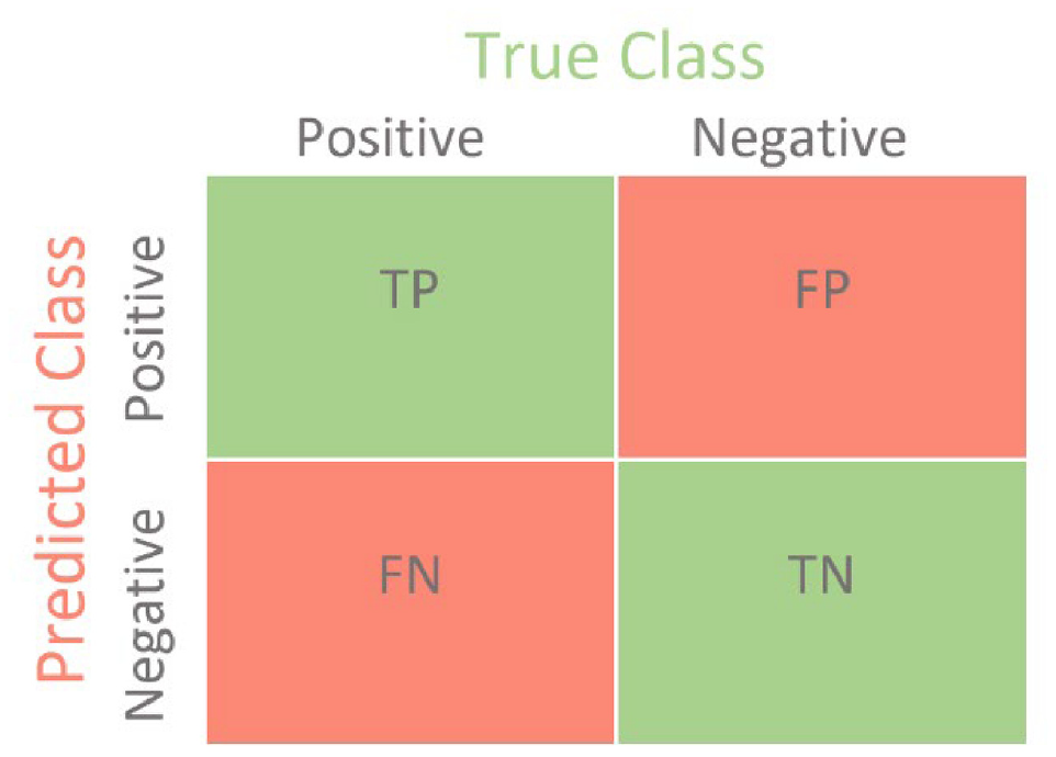
Confusion matrix for binary classification ( 48 ).

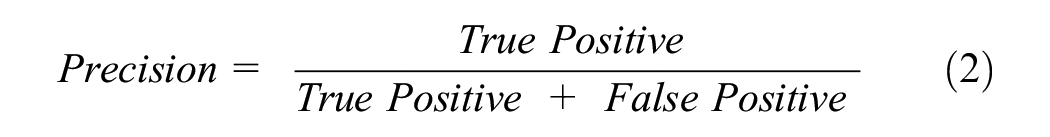
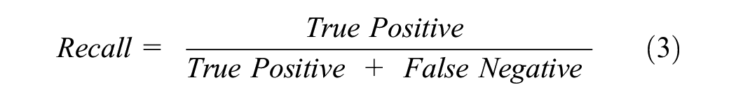
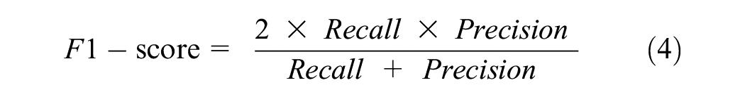
A classification report is simply a consolidated representation of precision, recall, F1-score, and support values of the testing dataset for the classifier model. The equations for precision, recall, and F1-score are given in Equations 2–4. The macro average in the classification report indicates the mean value of the evaluation parameters (precision, recall, and F1-score). However, the weighted average in the classification report indicates the weighted value of the evaluation parameter by multiplying the respective proportion of each class in the test dataset. Accuracy is a ratio of correctly predicted observations to total observations (Equation 5). In this research, the K-fold cross-validation technique is used with K = 10. The use of cross-validation helps to eliminate overfitting and underfitting scenarios. It also generalizes the model accuracy for any independent data ( 49 ). A classification model must have high accuracy, high precision, high recall, and high F1-score values to be called a high-performance classifier ( 48 ).

The algorithms described above were implemented using Python version 3.9.7:

Precision = \frac{True Positive}{True Positive + False Positive}

(2)

Recall = \frac{True Positive}{True Positive + False Negative}

(3)

F 1 - score = \frac{2 \times Recall \times Precision}{Recall + Precision}

(4)

\begin{matrix} Accuracy = \frac{True Positive + True Negative}{True Positive + False Positive + False Negative + True Negative} \end{matrix}

(5)

Hotspot Analysis of HRGC Crashes

Hotspot analysis is an advanced technique to identify hotspot locations using incident/crash data. This approach is superior to existing techniques for identifying crash frequency, rate, and density. In this research, hotspot analysis was conducted by incorporating two tools included in ArcGIS software: (i) spatial autocorrelation (Moran’s I method) and (ii) optimized hotspot analysis.

Spatial Autocorrelation (Moran’s I Method)

The spatial autocorrelation method uses global Moran’s I statistics, which consider feature values and location coordinates. Moran’s I was one of the earliest measures of spatial autocorrelation globally and is still used to assess spatial autocorrelation (Equation 6). The spatial autocorrelation tool provides results that include Moran’s I, Z-score, p-value, and so forth ( 50 ). Moran’s I helps identify spatial patterns such as random, dispersed, or clustered, while the Z-score and p-value help determine statistical significance and reject or accept the null hypothesis ( 19 ). Moran’s I can be calculated using the following equation:

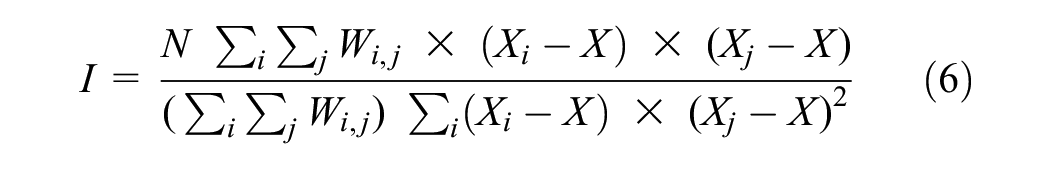
I = \frac{N \sum_{i} \sum_{j} W_{i, j} \times (X_{i} - X) \times (X_{j} - X)}{(\sum_{i} \sum_{j} W_{i, j}) \sum_{i} (X_{i} - X) \times {(X_{j} - X)}^{2}}

(6)

where N is the number of samples, X_i is the variable value at one location, X_j is the variable value at another location, X is the variable’s mean, and W_ij is a weight that compares locations i and j.

A Moran’s I value near +1 indicates clustering (positive spatial autocorrelation), and that near −1 indicates dispersion (negative spatial autocorrelation); a value of zero indicates a random (no spatial autocorrelation) distribution. In some cases, when the Z-score is extensive, but the significance value indicates rejection of the null hypothesis, Moran’s I needs to be assessed. The result displays a clustered pattern if the Moran’s I value is greater than 0 and a dispersed pattern if the Moran’s I value is less than 0 ( 19 ).

Optimized Hotspot Analysis

Optimized hotspot analysis is an ArcGIS software tool that helps search for the region with a high concentration of occurrences within a defined limit ( 19 ). Optimized hotspot analysis is similar to the hotspot analysis tool but uses a parameter from the input data to run Getis-Ord Gi* statistics, such as counts of crashes and counts of fatalities. The results provide statistically significant spatial clusters of the hotspots (high-value points) and coldspots (low-value points). This tool operates by examining each characteristic and considering its surrounding feature points. The outcome of optimized hotspot analysis gives a GiZScore and GiPValue for every sample of the dataset. These values help analyze the statistical significance and spatial clustering of the samples using Equations 7–9. The features with a high GiZScore and a low GiPValue indicate hotspots or high-value clustering locations, while features with a low GiZScore and low GiPValue indicate coldspots or low-value clustering locations ( 19 , 51 ):

G_{i}^{*} = \frac{\sum_{j = 1}^{n} w_{i, j} x_{j} - X \sum_{j = 1}^{n} w_{i, j}}{S \sqrt{\frac{n \sum_{j = 1}^{n} {w_{i, j}}^{2} - {(\sum_{j = 1}^{n} w_{i, j})}^{2}}{n - 1}}}

(7)

X = \frac{\sum_{j = 1}^{n} x_{j}}{n}

(8)

S = \sqrt{\frac{\sum_{j = 1}^{n} {x_{j}}^{2}}{n} - {(X)}^{2}}

(9)

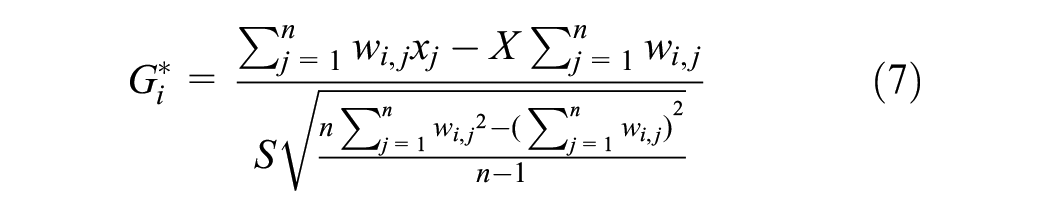
where $G_{i}^{*}$ is the Z-score for analysis, $x_{j}$ is the attribute value of feature j, $w_{i, j}$ is the spatial weight between features i and j, n is the total number of features, X is the mean center, and S is the standard deviation of all measurements.

Results

Feature Selection for HRGC Crash Data

Figure 4 shows the importance of each feature of the HRGC crash dataset generated by the ExtraTrees classifier. “Vehicles_Daily” emerges as the most influential feature, while “Access” exhibits the least impact on predicting the HRGC crashes using the classifier. The results shows similarity with the results of previously conducted studies ( 11 , 12 ).

Figure 4.

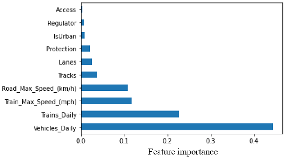
Feature importance for highway railroad grade crossing crash causes.

Feature Selection for Severity of Casualties in HRGC Crash Data

Figure 5 shows the importance for each feature with respect to severity of casualties associated with HRGC crashes as obtained by the extra trees classifier model. “Train_Speed_MPH” emerges as the most influential feature, while “NumberTrainsInvolved” exhibits the least impact on predicting the severity of casualties using the classifier. The results are in alignment with studies that were previously conducted ( 14 , 15 ). Also, the results here unveiled some important factors, such as occurrence hour (OccHour), vehicle type (VehicleTypeID), and season (Season), which were not identified in the previously conducted studies of HRGC safety.

Figure 5.

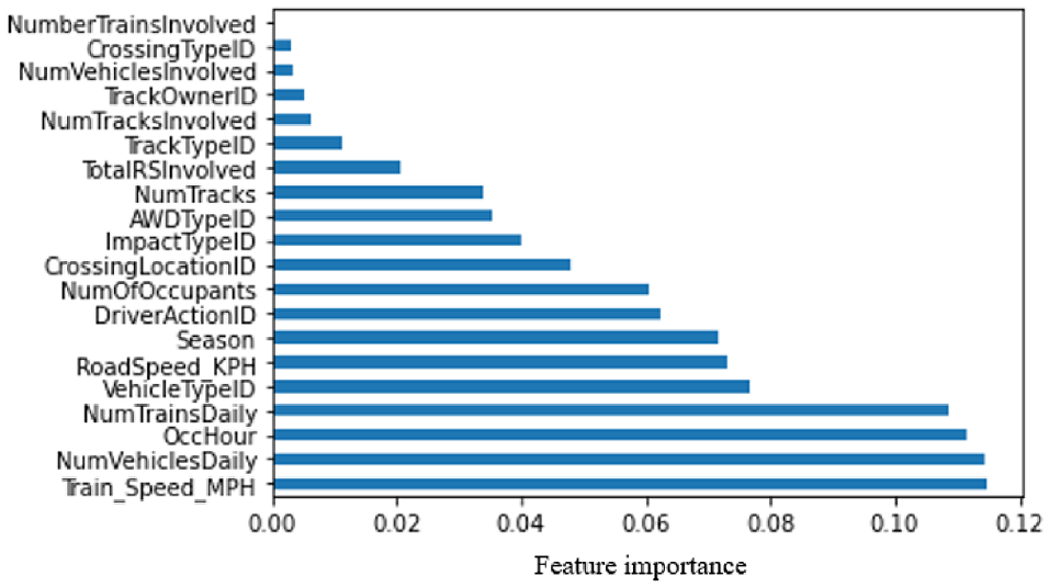
Feature importance for the severity of casualty causes.

Analysis of Results of the Classification Model of HRGC Crashes

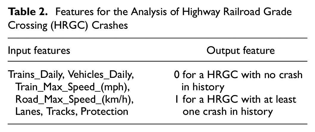
The HRGC crashes classification model was developed using features obtained from the feature selections, with the feature importance of each feature (Figure 4) considered in the model. The model accuracies were compared using a different number of features (based on the output of the ExtraTrees classifier) to obtain the optimum number of features for the classification model. The highest accuracy was obtained with the top seven features of the dataset, as reported in Table 2.

Table 2.

Features for the Analysis of Highway Railroad Grade Crossing (HRGC) Crashes

Input features	Output feature
Trains_Daily, Vehicles_Daily, Train_Max_Speed_(mph), Road_Max_Speed_(km/h), Lanes, Tracks, Protection	0 for a HRGC with no crash in history 1 for a HRGC with at least one crash in history

The classifiers were then evaluated using the mean accuracy of the classifier models (value of accuracy after K-fold cross-validation) ( 17 ). The highest mean accuracy value was obtained with XGBoost (0.90), followed by the RF (0.87) and AdaBoost (0.82) classifiers.

Performance parameters (precision, recall, and F1-score) for the XGBoost classifier are reported in Table 3. Both classes (0 and 1) show high accuracy, precision, recall, and F1-score with the XGBoost classifier.

Table 3.

Classification Report for the XGBoost Classifier for Highway Railroad Grade Crossing Crashes

Class	Precision	Recall	F1-score	Support
0 (no crashes)	0.95	0.98	0.96	3718
1 (at least 1 crash)	0.98	0.95	0.96	3718
Accuracy	NA	NA	0.96	7436
Macro avg.	0.96	0.96	0.96	7436
Weighted avg.	0.96	0.96	0.96	7436

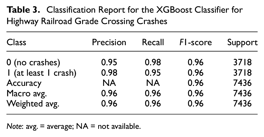
Note: avg. = average; NA = not available.

Analysis of Results of the Classification Model of the Severity of Casualties Associated with HRGC Crashes

The classification model was developed using features obtained from the feature selections, with the feature importance of each feature (Figure 5) considered in the model. The model accuracies were again compared using a different number of features (based on the output of the ExtraTrees classifier) to obtain the optimum number of features for the classification model. The highest accuracy was obtained with the top 11 features of the dataset, as reported in Table 4.

Table 4.

Features for the Analysis of the Severity of Casualties Associated with Highway Railroad Grade Crossing (HRGC) Crashes

Input features	Output feature
Season, OccHour, ImpactTypeID, CrossingLocationID, NumTrainsDaily, NumVehiclesDaily, RoadSpeed_KPH, DriverActionID, NumOfOccupants, VehicleTypeID, Train_Speed_MPH	0 for a HRGC crash with no serious injuries 1 for a HRGC crash with at least one serious injury 2 for a HRGC crash with at least one fatality

The classifiers were then evaluated using the mean accuracy of the classifier models (value of accuracy after K-fold cross-validation) ( 17 ). The highest accuracy was obtained with XGBoost (0.79), followed by the RF (0.75) and AdaBoost (0.53) classifiers.

The performance parameters (precision, recall, and F1-score) for the XGBoost classifier are reported in Table 5. All three classes (0, 1, and 2) show high accuracy, precision, recall, and F1-score with the XGBoost classifier.

Table 5.

Classification Report for XGBoost Classifier for the Severity of Casualties Associated with Highway Railroad Grade Crossing Crashes

	Precision	Recall	F1-score	Support
0 (no serious injuries)	0.80	0.74	0.77	77
1 (at least one serious injury)	0.87	0.88	0.86	77
2 (at least one fatality)	0.81	0.86	0.84	76
Accuracy	NA	NA	0.83	230
Macro avg.	0.83	0.83	0.83	230
Weighted avg.	0.83	0.83	0.83	230

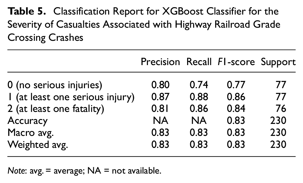
Note: avg. = average; NA = not available.

Results of Hotspot Analysis

The hotspot analysis of the HRGC crashes was conducted using the HRGC inventory dataset. The dataset contained crash counts at different HRGCs across the rail network with Global Positioning System (GPS) coordinates of each HRGC. The spatial autocorrelation of the dataset resulted in a z-score value of 8.1851, a p-value of zero, and Moran’s I more significant than zero (0.0116), which together indicate positive spatial autocorrelation and spatial clustering of HRGC crashes in the rail network ( 52 ). The data are distributed as clusters for the rail network, which can be helpful for further analysis of causal factors of HRGC crashes for each cluster.

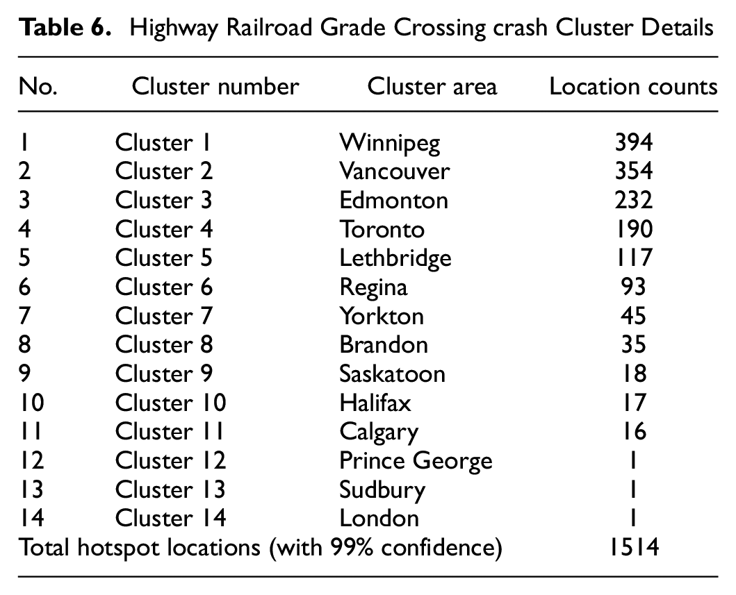
After obtaining the clustering distribution of HRGC crashes, optimized hotspot analysis was applied. The results of the optimized hotspot tool identified a total of 1514 hotspot locations (with 99% confidence) of HRGC crashes in Canada’s rail network (Figure 6).

Figure 6.

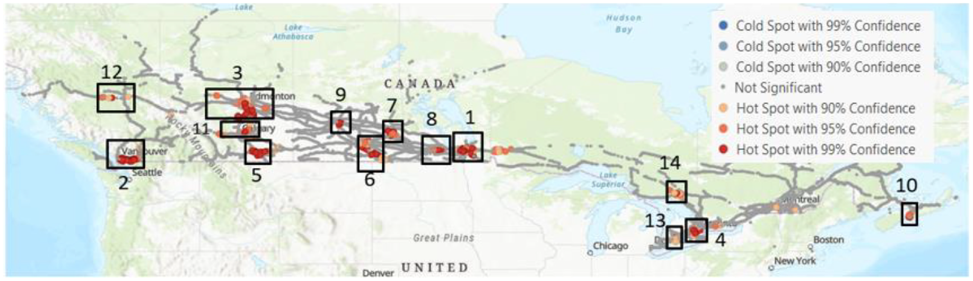
Hotspot locations for highway railroad grade crossing crashes with cluster number.

The details of hotspot locations were used to define different clusters based on their location across the rail network (Table 6).

Table 6.

Highway Railroad Grade Crossing crash Cluster Details

No.	Cluster number	Cluster area	Location counts
1	Cluster 1	Winnipeg	394
2	Cluster 2	Vancouver	354
3	Cluster 3	Edmonton	232
4	Cluster 4	Toronto	190
5	Cluster 5	Lethbridge	117
6	Cluster 6	Regina	93
7	Cluster 7	Yorkton	45
8	Cluster 8	Brandon	35
9	Cluster 9	Saskatoon	18
10	Cluster 10	Halifax	17
11	Cluster 11	Calgary	16
12	Cluster 12	Prince George	1
13	Cluster 13	Sudbury	1
14	Cluster 14	London	1
Total hotspot locations (with 99% confidence)			1514

Discussion of Results

Causes of HRGC Crashes

According to Figure 4, the most important causal factor of HRGC crashes is “Vehicles_Daily,” which is the number of road vehicles per day over a given HRGC. An assessment of crossing inventory data shows that the probability of HRGC crashes increases as the number of daily vehicles increases for a given HRGC. The second most influential factor for HRGC crashes is “Trains_Daily,” the number of trains per day over a given HRGC. Table 7 shows the probability of HRGC crashes for different daily train counts and indicates a positive relation with daily train counts. The probability of a HRGC crash is determined by dividing the number of HRGCs with a crash history within a specific range of causal factors by the total number of HRGCs within that same range. The increased probability of HRGC crashes with higher traffic can be attributed to the more frequent meet up of vehicles and trains on the HRGC sites.

Table 7.

Effect of Factors of Highway Railroad Grade Crossing crash Probability

Daily vehicle traffic		Daily train traffic		Rail tracks
Vehicles	Probability of crash	Trains	Probability of crash	Tracks	Probability of crash
<1000	0.0219	<1	0.0090	1	0.0263
1000–2000	0.0511	1–2	0.0153	2	0.0499
2000–3000	0.0492	2–3	0.0176	3	0.0441
3000–4000	0.0833	3–4	0.0311	>3	0.0617
4000–5000	0.0855	4–5	0.0264
5000–10,000	0.0785	5–10	0.0473
>10,000	0.0851	>10	0.0953
Train speed		Road speed		Highway lanes
Train speed (mph)	Probability of crash	Road speed (km/h)	Probability of crash	Lane	Probability of crash
<10	0.0204	<20	0.0108	1	0.0125
10–25	0.0194	21–40	0.0196	2	0.0318
25–40	0.0281	41–60	0.0383	3	0.0345
40–60	0.0476	61–80	0.0300	4	0.0836
60>	0.0477	>80	0.0415	>4	0.1023

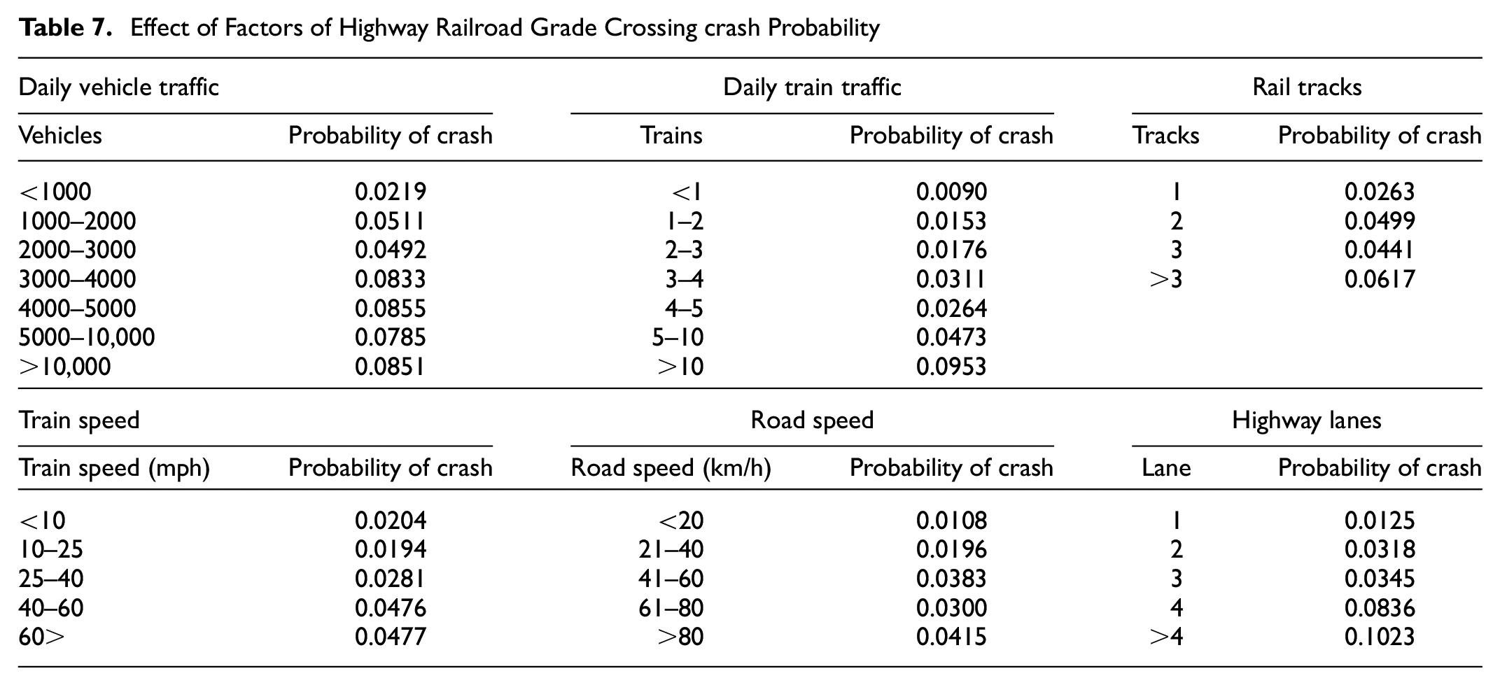
Train_Max_Speed_(mph) is the third most influential causal factor for HRGC crashes. The fourth most important causal factor for HRGC crashes is Road_Speed_(km/h). On assessment of HRGC inventory data, the probability of HRGC crashes increases with increased train speed and road speed. The shorter time available for evaluating the HRGC site’s conditions and making safe decisions about the HRGC’s crossover can be attributed to the increased probability of HRGC crashes at higher speeds (Table 7).

The fifth most important causal factor of HRGC crashes is “Tracks,” which means the number of rail tracks at a HRGC. Table 7 shows that the probability of HRGC crashes rises with an increase in track numbers at HRGCs. “Lanes” on the highway are the sixth most important cause of HRGC crashes. Similar to the number of rail tracks, the probability of HRGC crashes increases with an increase in the number of lanes at HRGCs. The longer time required for vehicles to traverse the HRGC can be attributed for the greater likelihood of HRGC crashes with a higher track number ( 53 ). Similar to this, more vehicles are exposed on the HRGCs with more highway lanes than in those with fewer highway lanes, which increases the probability of HRGC crashes (Table 7).

“Protection” is the seventh most important causal factor for HRGC crashes, and refers to the type of protection device installed at a given HRGC. The data from Canadian railways show 45% of HRGC crashes happen at passive crossings, followed by 30% at crossings equipped with flashlights, gates, and bells, and 25% at crossings equipped with flashlights and gates. These data indicate that protection devices at a given HRGC help to reduce the number of HRGC crashes.

Causes of Severe Casualties Associated with HRGC Crashes

The most important causal factor for the severity of casualties associated with HRGC crashes is “Train_Speed_MPH.”Figure 7 shows that the probability of crashes at HRGCs with fatalities and serious injuries increases with train speed. The figure also shows the probability of a serious injury crash is less at higher train speeds compared to the probability of a fatal crash, likely because of higher train speeds resulting in more fatalities.

Figure 7.

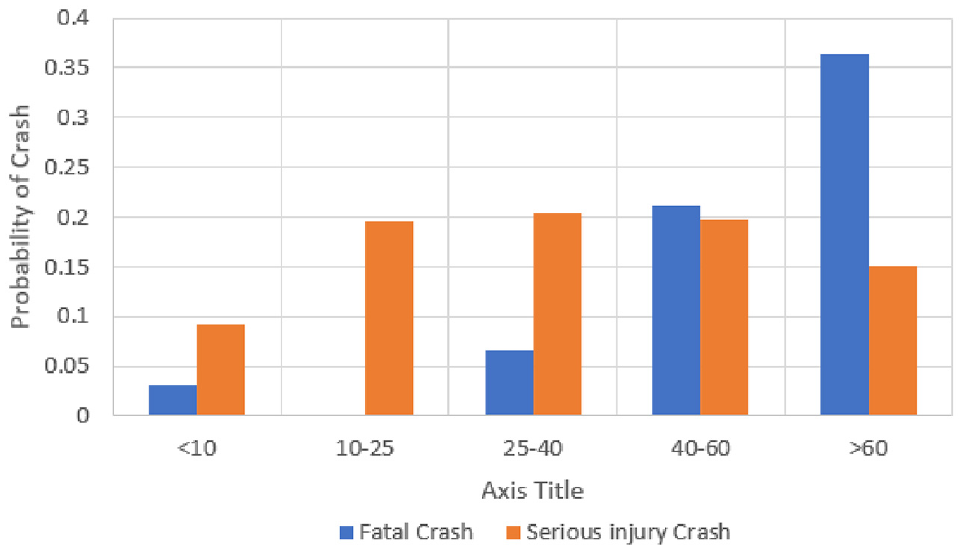
Effect of train speed on the probability of severe injury or fatality associated with a highway railroad grade crossing crash.

The second most important causal factor for the severity of casualties associated with HRGC crashes is “NumTrainsDaily,” which indicates the number of trains passing over a given HRGC. Figure 8 indicates that the probability of a fatal crash increases with an increase in daily trains, with the highest probability of a fatal crash associated with >25 daily trains. The probability of serious injury crashes varies with daily train count, with the highest probability associated with 5–10 daily trains at HRGCs.

Figure 8.

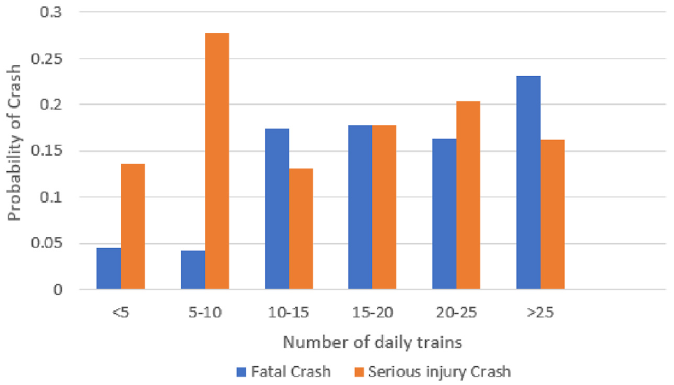
Effect of the number of daily trains on the probability of severe injury or fatality associated with a crash at a highway railroad grade crossing.

“NumVehiclesDaily” is the third influential causal factor for the severity of casualties associated with HRGC crashes and refers to the number of vehicles crossing over a given HRGC. Figure 9 shows the probabilities of fatal and serious injury crashes, which both vary over the range of daily vehicles. The highest probability of a fatal crash is observed for <1000 daily vehicles, and the highest probability of serious injury crashes is observed for 1000–2000 daily vehicles.

Figure 9.

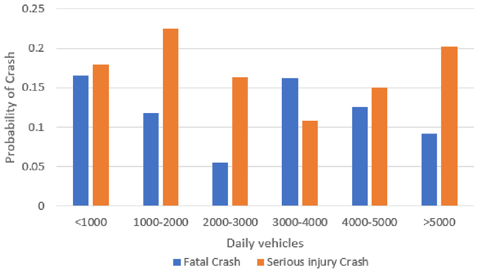
Effect of number of daily vehicles on the probability of severe injury or fatality associated with a highway railroad grade crossing crash.

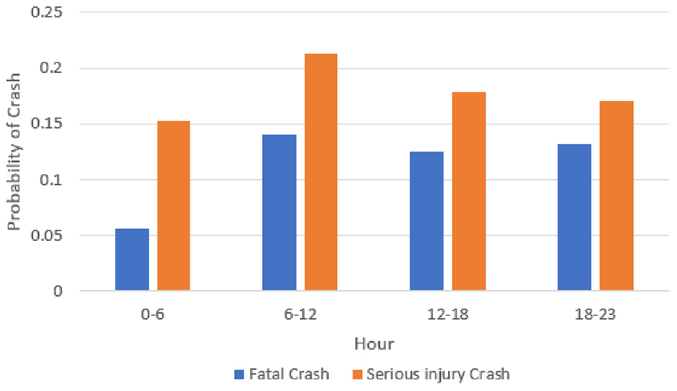
“OccHour,” the hour of the day when a crash occurred, is the fourth most important causal factor for the severity of casualties associated with HRGC crashes. Figure 10 shows that the probability of fatal and serious injury crashes varies with the time of day, and is highest between 06:00 and 18:00. This is likely because of factors such as high volumes of commuter traffic, traffic jams/impatience, and sleepiness in the late afternoon. A high probability of fatal and serious injury crashes is observed between 18:00 and 23:00, which is likely because of factors such as low visibility, slower reaction time, and tiredness ( 54 ).

Figure 10.

Effect of hour of the day on the probability of severe injury or fatality associated with a highway railroad grade crossing crash.

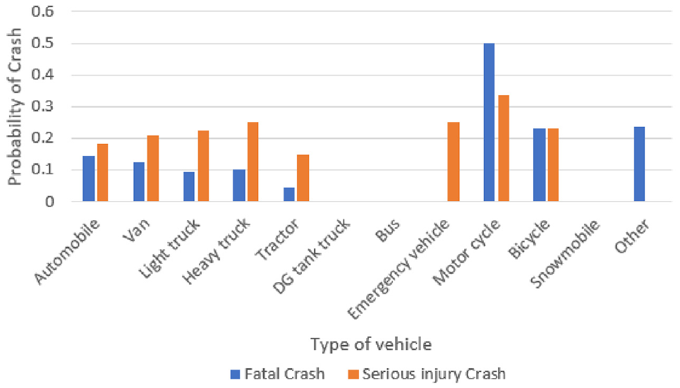
The fifth most influential causal factor is “VehicleTypeID,” which refers to the type of vehicle involved in the crash. Figure 11 shows the probability of a fatal crash is highest for motorcycles, followed by bicycles and automobiles, and the probability of a serious injury crash is highest for motorcycles, followed by heavy trucks and bicycles.

Figure 11.

Effect of vehicle type on the probability of severe injury or fatality associated with a highway railroad grade crossing crash.

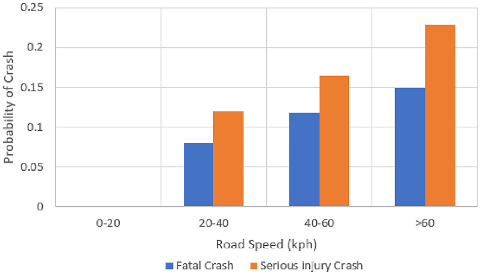
“RoadSpeed_KPH” is the sixth most important feature and refers to the maximum road speed at a HRGC. Figure 12 indicates that the probability of both fatal and serious injury crashes increases with maximum road speed.

Figure 12.

Effect of road speed on the probability of severe injury or fatality associated with a highway railroad grade crossing crash.

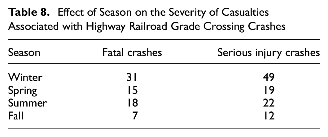
The seventh most important causal factor that affects the severity of casualties associated with HRGC crashes is “Season.”Table 8 shows that the highest number of fatal and serious injury crashes happens in winter conditions and the lowest number in the fall. Weather conditions such as low visibility, the presence of snow, and poor road conditions are contributing factors to high-severity crashes in the winter ( 55 ).

Table 8.

Effect of Season on the Severity of Casualties Associated with Highway Railroad Grade Crossing Crashes

Season	Fatal crashes	Serious injury crashes
Winter	31	49
Spring	15	19
Summer	18	22
Fall	7	12

Discussion of Hotspot Analysis Results

Figure 6 and Table 6 show major crash-prone clusters near major cities. The top three HRGC crash hotspot clusters are located near Winnipeg (cluster-1), Vancouver (cluster-2), and Edmonton (cluster-3), with 394, 354, and 232 HRGC crash hotspot locations, respectively.

The characteristics of cluster-1 were examined based on the HRGC features examined earlier (Feature Selection for HRGC Crash Data section). This assessment of cluster characteristics shows that of these HRGCs: (1) 50% were equipped with passive protection and 50% with active protection equipment; (2) 22% handle vehicle traffic volumes greater than 5000 vehicles per day; (3) 29% handle more than 10 trains per day; (4) 40% have a road speed of more than 60 km/h; (5) 20% have a train speed of more than 60 mph; (6) 21% have more than one track; and (7) 14% have more than two lanes. Targeting these features from the given analysis can help reduce the crashes at HRGCs in cluster-1.

Recommendations

The ML algorithms highlight how railway, highway, environmental, and human factors contribute to HRGC crashes and the severity of associated casualties. Important railway and road factors discussed above include maximum train speed, number of tracks, daily train volumes, lanes, maximum road speed, and traffic volume. Environmental factors such as season, hour of the day, and visibility also contribute to HRGC crashes and consequences. Human factors include intentional attempts to cross, distracted/confused drivers, visibility obstructions, fatigue, slip of memory/attention, cognitive and emotional distractions, and so forth ( 56 , 57 ).

Based on the results of this study, possible strategies to reduce HRGC crashes and related casualties are as follows.

Installing gates and automatic railway-controlled crossings can restrict vehicles from entering the tracks ( 58 ). Upgrading passive crossings to active crossings by installing flashing lights, bells, and gates can help to reduce HRGC crashes ( 12 ). In addition, installing four-quadrant and median barriers reduce the chances of crashes at HRGCs and reduce severity in the case of crashes ( 59 ). Table 9 shows the effects of crossing features on HRGC crashes and the severity of casualties.

Developing grade separations for crossings that handle high daily vehicle and train traffic is a good solution to reduce the risk of crashes between trains and vehicles ( 60 , 61 ). Grade separation showed a 100% decrease in injuries and fatalities ( 62 ).

Advanced warning devices can be implemented to address the effects of many highway lanes and tracks at HRGCs ( 53 ). Carroll and Warren ( 63 ) recommend an automated photo and video enforcement system to help investigate vehicle users’ compliance with existing warning infrastructure at HRGCs. This system has reduced HRGC-related violations by 34%–92%.

Reduction of train and vehicle speeds during their approach to high-risk HRGCs can reduce HRGC crashes and the severity of associated casualties ( 64 ).

Reduced lighting and/or hindrance to recognizing the incoming train are factors in HRGC crashes. Thus, installing a lighting source and clearing obstructions from the nearby area could reduce the risk of HRGC crashes ( 60 ). The provision of lighting sources at HRGCs resulted in a reduction of nighttime crashes by 52% ( 62 ).

Pavement strips/rumble strips near crossings are noticeable and effective in helping drivers recognize upcoming crossings ( 5 ).

Education through campaigns, for drivers and pedestrians, about traffic discipline and the consequences of HRGC crashes to individuals and the railway can be effective ( 56 ). Awareness campaigns have resulted in a 15% reduction in HRGC crashes and a 19% reduction in fatalities associated with HRGC crashes ( 62 ).

Table 9.

Effect of Crossing Features on Crossing Crashes and Fatalities ( 62 )

No.	Crossing feature	Effect
1	Flashing lights	1. Reduction by 64% in HRGC crash crashes in contrast to HRGCs with only crossbucks.
1	Flashing lights	2. Reduction in injuries by 84% and reduction in fatalities by 83% when compared with only crossbucks.
2	Lights and gates (2) with flashing lights	1. Reduction by 88% in HRGC crash crashes compared to HRGCs with only crossbucks.
		2. Reduction in injuries by 93% and reduction in fatalities by 100% when compared with only crossbucks.
		3. Reduction by 44% in HRGC crash crashes compared to HRGCs with flashing lights.
3	Median barrier	Reduction by 80% in violations compared to 2-gate system.
4	Long arm gates (3/4 of road coverage)	Reduction by 67%–84% in violations compared to 2-gate system.
5	4-quadrant gate system	Reduction in violations by 82% compared to 2-gate system.
6	4-quadrant gate system+median barriers	Reduction in violations by 92% compared to 2-gate system.

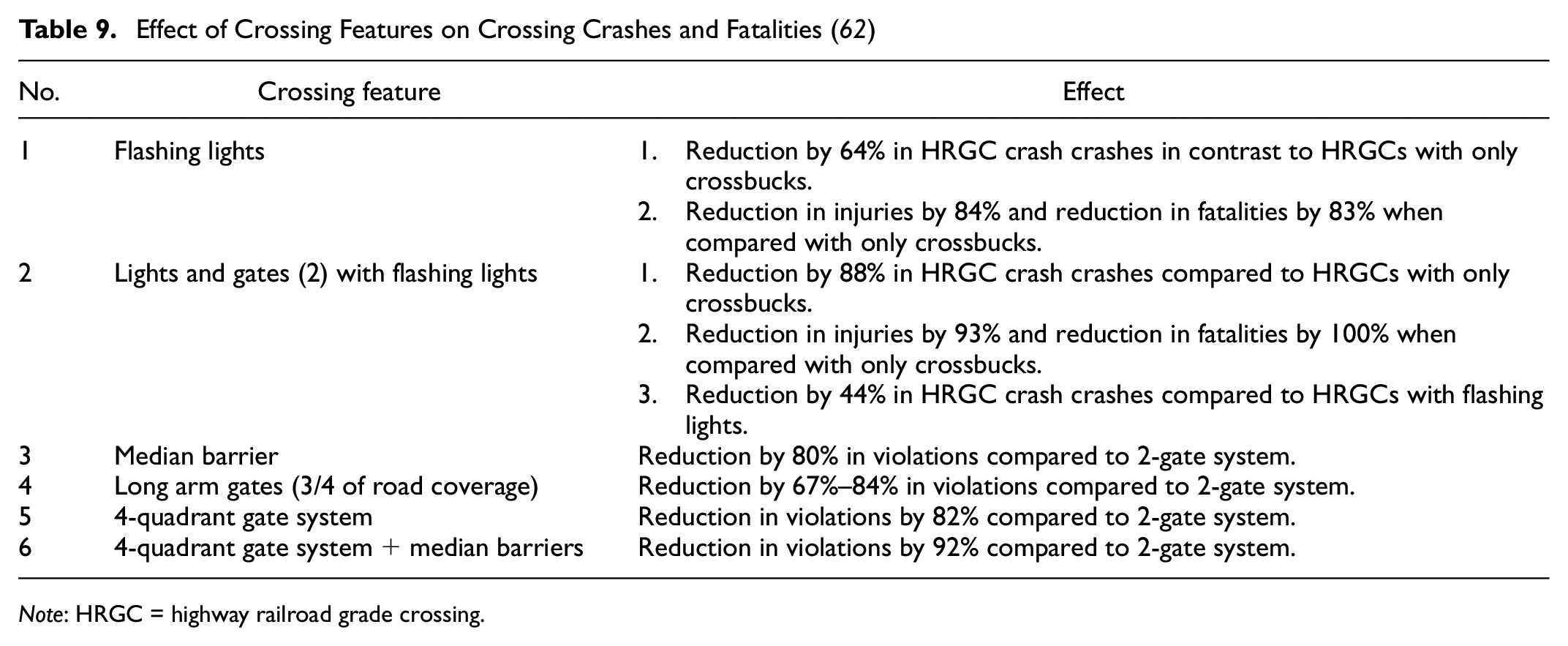
Note: HRGC = highway railroad grade crossing.

Conclusion

HRGCs are regarded as high-risk areas on railway networks because of the catastrophic consequences that can result from HRGC crashes. Thus, transportation authorities place a great focus on safety at HRGCs. This study identified the major causal factors for HRGC crashes and the severity of casualties associated with HRGC crashes in Canada. The results indicate that high train traffic, high vehicle traffic, high highway speed, and high track speed are major factors that contribute to HRGC crashes, while occurrence hour, type of vehicle, high train traffic, high vehicle traffic, high highway speed, and high train speed are major factors that contribute to the severity of casualties associated with HRGC crashes. The use of ensemble classification ML models has provided better prediction results and managed to handle the complex relationship among the variables used for modeling. The ML models help predict HRGC crashes and the associated severity of casualties by employing supervised ML algorithms. These supervised ML models are handy tools for authorities to interpret the data and re-apply using updated data whenever required in the future. The causes identified in this research match with the same study identified in the introduction section. In addition, optimized hotspot analysis using ArcGIS software recognized the spatial patterns of HRGC crashes in Canada’s rail network. Identifying such HRGC crash hotspot locations will allow authorities to target high-risk crash-prone areas of the railway network. Using these findings of high-risk HRGC locations, authorities can assess high-risk HRGC locations, as each HRGC is unique. Subsequently, the authorities will assess the suitability of these recommendations and make informed decisions with respect to the implementation of which recommendation for improving the safety of HRGCs.

The findings of this research can benefit authorities and policymakers concerning decision-making, allocating resources, and implementing countermeasures to reduce the number of HRGC crashes and the severity of associated casualties in Canada’s rail network. The study provided a range of recommendations to enhance HRGC safety; choosing the most suitable recommendation requires careful consideration. Implementing these recommendations necessitates a separate study that assesses the various available options and identifies the most effective approach to reducing risks at HRGCs and improving safety. This could potentially serve as a topic for future research.

However, this study is not without limitations. The source datasets used for this research had many empty features because of poor reporting, and thus were excluded from the datasets used in the analysis. As such, the analysis may not have identified all causal factors for HRGC crashes and the severity of associated casualties. Furthermore, the classification model datasets did not consider human-related features, such as driver experience, state (physical/mental), and gender. Thus, future research should investigate the role of human factors in HRGC crashes and the severity of associated casualties to provide more insight and help improve the safety of HRGCs in the rail network. The HRGC study carried out in this research is specific to the Canadian railway network. The ML models and spatial correlation techniques relied on data pertaining to the Canadian railway network. Therefore, the models in this study are intrinsically tied to the dataset. If a similar study were to be conducted using data from different railway networks, it would be necessary to retrain the models with a new dataset to accurately represent the characteristics of those specific railway networks.

Footnotes

Authors Contributions

The authors confirm contribution to the paper as follows: study conception and design: P. Rana, F. Sattari, L. Lefsrud, M. Hendry; data collection: P. Rana, F. Sattari, L. Lefsrud, M. Hendry; analysis and interpretation of results: P. Rana, F. Sattari, L. Lefsrud, M. Hendry; draft manuscript preparation: P. Rana. All authors reviewed the results and approved the final version of the manuscript.

Declaration of Conflicting Interests

The author(s) declared no potential conflicts of interest with respect to the research, authorship, and/or publication of this article.

Funding

The author(s) disclosed receipt of the following financial support for the research, authorship, and/or publication of this article: Funding for this study has been provided through the Canadian Rail Research Laboratory at the University of Alberta with funding provided by Transport Canada (T8009-210202), the National Research Council of Canada (989894) and the National Sciences and Engineering Research Council of Canada (IRCPJ 544435).

ORCID iDs

Fereshteh Sattari

lianne Lefsrud

References

Railway Association of Canada. Canada’s Freight Railways: Moving the Economy. Railway Association of Canada. 2023. https://www.railcan.ca/101/canadas-freight-railways-moving-the-economy/. Accessed February 14, 2023.

Ouedraogo

K. A.

Beugin

El-Koursi

E. M.

Clarhaut

Renaux

Lisiecki

Toward an Application Guide for Safety Integrity Level Allocation in Railway Systems. Risk Analysis, Vol. 38, No. 8, 2018, pp. 1634–1655.

Transport Canada. Rail Safety in Canada. 2021. https://tc.canada.ca/en/rail-transportation/rail-safety-canada. Accessed October 24, 2022.

Government of Canada. Grade Crossings Inventory. 2022. https://open.canada.ca/data/en/dataset/d0f54727-6c0b-4e5a-aa04-ea1463cf9f4c. Accessed August 9, 2022.

Tey

L. S.

Wallis

Cloete

Ferreira

Modelling Driver Behaviour Towards Innovative Warning Devices at Railway Level Crossings. Accident Analysis & Prevention, Vol. 51, 2013, pp. 104–111.

Tolliver

Accident Prediction Model for Public Highway-Rail Grade Crossings. Accident Analysis & Prevention, Vol. 90, 2016, pp. 73–81.

Transport Canada. Enhancing Rail Safety in Canada: Working Together for Safer Communities. 2018. https://tc.canada.ca/sites/default/files/migrated/enhancing_rail_safety_canada_working_together_safer_communities.pdf. Accessed January 6, 2023.

Transportation Safety Board of Canada (TSB). Rail Transportation Occurrences in 2021. 2021. http://www.tsb.gc.ca/eng/stats/rail/2021/sser-ssro-2021.html. Accessed September 15, 2022.

Federal Railroad Administration (FRA). Highway-Rail Grade Crossings Overview. 2019. https://railroads.dot.gov/program-areas/highway-rail-grade-crossing/highway-rail-grade-crossings-overview. Accessed January 16, 2023.

10.

Das

Kong

Lavrenz

S. M.

Jalayer

Fatal Crashes at Highway Rail Grade Crossings: A U.S. Based Study. International Journal of Transportation Science and Technology, Vol. 11, No. 1, 2022, pp. 107–117.

11.

Tolliver

Zheng

Highway-Rail Grade Crossing Traffic Hazard Forecasting Model. 2018. https://www.ugpti.org/resources/reports/downloads/mpc18-354.pdf. Accessed November 30, 2022.

12.

Mok

S. C.

Savage

Why Has Safety Improved at Rail-Highway Grade Crossings?

Risk Analysis, Vol. 25, No. 4, 2005, pp. 867–881.

13.

Brod

Gillen

A New Model for Highway-Rail Grade Crossing Accident Prediction and Severity. 2020. https://railroads.dot.gov/elibrary/new-model-highway-rail-grade-crossing-accident-prediction-and-severity. Accessed November 30, 2022.

14.

Brabb

D. C.

Vithani

Martin

In-Depth Data Analysis of Grade Crossing Accidents Resulting in Injuries and Fatalities. 2017. https://railroads.dot.gov/elibrary/depth-data-analysis-grade-crossing-accidents-resulting-injuries-and-fatalities. Accessed December 19, 2022.

15.

Soleimani

Leitner

Codjoe

Applying Machine Learning, Text Mining, and Spatial Analysis Techniques to Develop a Highway-Railroad Grade Crossing Consolidation Model. Accident Analysis & Prevention, Vol. 152, 2021, p. 105985.

16.

Zheng

Tolliver

Decision Tree Approach to Accident Prediction for Highway-Rail Grade Crossings: Empirical Analysis. Transportation Research Record: Journal of the Transportation Research Board, 2016. 2545: 115–122.

17.

Lasisi

Chen

Hybrid Machine Learning and Geographic Information Systems Approach — A Case for Grade Crossing Crash Data Analysis. Advances in Data Science and Adaptive Analysis, Vol. 12, No. 1, 2020, p. 2050003.

18.

Liang

The Analysis of Spatial Pattern and Hotspots of Aviation Accident and Ranking the Potential Risk Airports Based on GIS Platform. Journal of Advanced Transportation, Vol. 2018, 2018, pp. 1–12.

19.

Prasannakumar

Vijith

Charutha

Geetha

Spatio-Temporal Clustering of Road Accidents: GIS Based Analysis and Assessment. Procedia – Social and Behavioral Sciences, Vol. 21, 2011, pp. 317–325.

20.

Mulugeta Tola

Gebissa

Identifying Black Spot Accident Zones Using a Geographical Information System on Kombolcha-Dessie Road in Ethiopia. International Journal of Sciences: Basic and Applied Research (IJSBAR), Vol. 48, No. 1, 2019, pp. 66–79.

21.

Heydari

Developing Safety Performance Functions for Railway Grade Crossings: A Case Study of Canada. Proc., ASME/IEEE Joint Rail Conference, American Society of Mechanical Engineers, New York, 2015, p. V001T06A017.

22.

Transportation Safety Board of Canada. Dataset from January 1983 – Transportation Safety Board of Canada. 2020. https://www.bst-tsb.gc.ca/eng/stats/rail/data-5.html. Accessed August 26, 2022.

23.

Zhu

Hou

Application of Machine Learning Techniques for Predicting the Consequences of Construction Accidents in China. Process Safety and Environmental Protection, Vol. 145, 2021, pp. 293–302.

24.

Ajayi

Oyedele

Owolabi

Akinade

Bilal

Davila Delgado

J. M.

Akanbi

Deep Learning Models for Health and Safety Risk Prediction in Power Infrastructure Projects. Risk Analysis, Vol. 40, No. 10, 2020, pp. 2019–2039.

25.

Oba

Sato

M. A.

Takemasa

Monden

Matsubara

K. I.

Ishii

A Bayesian Missing Value Estimation Method for Hene Expression Profile Data. Bioinformatics, Vol. 19, No. 16, 2003, pp. 2088–2096. https://academic.oup.com/bioinformatics/article/19/16/2088/242445. Accessed May 29, 2023.

26.

Arya

Sastry

G. H.

Motwani

Kumar

Zaguia

A Novel Extra Tree Ensemble Optimized DL Framework (ETEODL) for Early Detection of Diabetes. Front Public Health, Vol. 9, 2022, p. 797877.

27.

Gromski, P. S., Y. Xu, E. Correa, D. I. Ellis, M. L. Turner, and R. Goodacre. A Comparative Investigation of Modern Feature Selection and Classification Approaches for the Analysis of Mass Spectrometry Data. Analytica Chimica Acta, Vol. 829, 2014, pp. 1–8.

28.

Janecek

A. G. K.

Gansterer

W. N.

Demel

M. A.

Ecker

G. F.

On the Relationship Between Feature Selection and Classification Accuracy. Proc., JMLR: Workshop and Conference Proceedings4, 2008, pp. 90–105. http://proceedings.mlr.press/v4/janecek08a/janecek08a.pdf. Accessed January 15, 2023.

29.

Ali

R. H.

Abdulsalam

W. H.

The Prediction of COVID 19 Disease Using Feature Selection Techniques. Journal of Physics: Conference Series, Vol. 1879, 2021, p. 22083.

30.

Kwon

Sim

J. M.

Effects of Data Set Features on the Performances of Classification Algorithms. Expert Systems with Applications, Vol. 40, No. 5, 2013, pp. 1847–1857.

31.

J. L.

Application of Random-SMOTE on Imbalanced Data Mining. Proc., 4th International Conference on Business Intelligence and Financial Engineering, BIFE 2011, Wuhan, China, IEEE, New York, 2011, pp. 130–133.

32.

Ghofrani

Sun

Analyzing Risk of Service Failures in Heavy Haul Rail Lines: A Hybrid Approach for Imbalanced Data. Risk Analysis, Vol. 42, No. 8, 2022, pp. 1852–1871.

33.

Wei

Dunbrack

R. L.

The Role of Balanced Training and Testing Data Sets for Binary Classifiers in Bioinformatics. PloS One, Vol. 8, No. 7, 2013. https://pubmed.ncbi.nlm.nih.gov/23874456/. Accessed December 2, 2022.

34.

Tanha

Abdi

Samadi

Razzaghi

Asadpour

Boosting Methods for Multi-Class Imbalanced Data Classification: An Experimental Review. Journal of Big Data, Vol. 7, No. 1, 2020, pp. 1–47. https://link.springer.com/article/10.1186/s40537-020-00349-yAccessed November 5, 2022.

35.

Fernández

Garcia

Herrera

Chawla

N. V.

SMOTE for Learning from Imbalanced Data: Progress and Challenges, Marking the 15-Year Anniversary. Journal of Artificial Intelligence Research, Vol. 61, 2018, pp. 863–905. http://www.jair.org/index.php/jair/article/view/11192. Accessed May 29, 2023.

36.

Ramos-Pérez

Arnaiz-González

Á.

Rodríguez

J. J.

García-Osorio

When is Resampling Beneficial for Feature Selection with Imbalanced Wide Data?

Expert Systems with Applications, Vol. 188, 2022, pp. 957–4174. https://doi.org/10.1016/j.eswa.2021.116015.

37.

Kürs

Uçar

Nour

Sindi

Polat

The Effect of Training and Testing Process on Machine Learning in Biomedical Datasets. Mathematical Problems in Engineering, Vol. 2020, 2020, pp. 1–17. https://doi.org/10.1155/2020/2836236.

38.

Zheng

Ren

Zhou

Keramati

Tolliver

Huang

A Gradient Boosting Crash Prediction Approach for Highway-Rail Grade Crossing Crash Analysis. Journal of Advanced Transportation, Vol. 2020, 2020, pp. 1–10. https://doi.org/10.1155/2020/6751728.

39.

Vijaya

Sivasankar

Computing Efficient Features Using Rough Set Theory Combined with Ensemble Classification Techniques to Improve the Customer Churn Prediction in Telecommunication Sector. Computing, Vol. 100, No. 8, 2018, pp. 839–860.

40.

Chen

Basic Ensemble Learning (Random Forest, AdaBoost, Gradient Boosting)- Step by Step Explained. Medium. 2019. https://towardsdatascience.com/basic-ensemble-learning-random-forest-adaboost-gradient-boosting-step-by-step-explained-95d49d1e2725. Accessed December 2, 2022.

41.

Nikulski

The Ultimate Guide to AdaBoost, Random Forests and XGBoost. Medium. 2020. https://towardsdatascience.com/the-ultimate-guide-to-adaboost-random-forests-and-xgboost-7f9327061c4f. Accessed August 13, 2022.

42.

Gupta

Chandrasekaran

A Study and Analysis of Machine Learning Techniques in Predicting Wine Quality. International Journal of Recent Technology and Engineering (IJRTE), Vol. 10, No. 1, 2021, pp. 314–319.

43.

T. K.

Kim

M. H.

A New Diverse AdaBoost Classifier. Proc., International Conference on Artificial Intelligence and Computational Intelligence, AICI 2010, Sanya, China, Vol. 1, 2010, pp. 359–363.

44.

Lin

Zheng

Han

Comparative Performance of Eight Ensemble Learning Approaches for the Development of Models of Slope Stability Prediction. Acta Geotechnica, Vol. 17, No. 4, 2022, pp. 1477–1502. https://link.springer.com/article/10.1007/s11440-021-01440-1. Accessed May 29, 2023.

45.

Kiangala

S. K.

Wang

An Effective Adaptive Customization Framework for Small Manufacturing Plants Using Extreme Gradient Boosting-XGBoost and Random Forest Ensemble Learning Algorithms in an Industry 4.0 Environment. Machine Learning with Applications, Vol. 4, 2021, p. 100024.

46.

Chen

Guestrin

XGBoost: A Scalable Tree Boosting System. Proc., ACM SIGKDD International Conference on Knowledge Discovery and Data Mining, August 13–17, 2016, ACM, New York, pp. 785–794.

47.

Shahrivari

Darabi

M. M.

Izadi

Phishing Detection Using Machine Learning Techniques. arXiv Preprint arXiv:2009.11116, 2020.

48.

Mohajon

Confusion Matrix for Your Multi-Class Machine Learning Model. Medium. 2020. https://towardsdatascience.com/confusion-matrix-for-your-multi-class-machine-learning-model-ff9aa3bf7826. Accessed September 11, 2022.

49.

Wong

T. T.

Yeh

P. Y.

Reliable Accuracy Estimates from k-Fold Cross Validation. IEEE Transactions on Knowledge and Data Engineering, Vol. 32, No. 8, 2020, pp. 1586–1594.

50.

Esri. Spatial Autocorrelation (Global Moran’s I) (Spatial Statistics)—ArcGIS Pro. 2020. https://pro.arcgis.com/en/pro-app/latest/tool-reference/spatial-statistics/spatial-autocorrelation.htm. Accessed November 19, 2022.

51.

Esri. How Hot Spot Analysis (Getis-Ord Gi*) Works—ArcGIS Pro. 2020. https://pro.arcgis.com/en/pro-app/latest/tool-reference/spatial-statistics/h-how-hot-spot-analysis-getis-ord-gi-spatial-stati.htm. Accessed November 19, 2022.

52.

Lakshmi

Srikanth

Arockiasamy

Identification of Traffic Accident Hotspots Using Geographical Information System (GIS). International Journal of Engineering and Advanced Technology (IJEAT), Vol. 9, No. 2, 2019, pp. 4429–4438. www.ijeat.org. Accessed November 11, 2022.

53.

Keramati

Tolliver

Wang

Geometric Effect Analysis of Highway-Rail Grade Crossing Safety Performance. Accident Analysis & Prevention, Vol. 138, 2020, p. 105470.

54.

Hao

Kamga

Wan

The Effect of Time of Day on Driver’s Injury Severity at Highway-Rail Grade Crossings in the United States. Journal of Traffic and Transportation Engineering (English Edition), Vol. 3, No. 1, 2016, pp. 37–50.

55.

Singh

Pasha

Khorram-Manesh

Goniewicz

Roshani

Dulebenets

M. A.

A Holistic Analysis of Train-Vehicle Accidents at Highway-Rail Grade Crossings in Florida. Sustainability (Switzerland), Vol. 13, No. 16, 2021, p. 105236.

56.

Sekasi

Solihu

Safety and Risk Analysis at Railway Crossings of North-South Addis Ababa Light Rail. Smart and Resilient Transportation, Vol. 3, No. 3, 2021, pp. 266–282. http://creativecommons.org/licences/by/4.0/legalcode.

57.

Baysari

M. T.

McIntosh

A. S.

Wilson

J. R.

Understanding the Human Factors Contribution to Railway Accidents and Incidents in Australia. Accident Analysis & Prevention, Vol. 40, No. 5, 2008, pp. 1750–1757. https://pubmed.ncbi.nlm.nih.gov/18760104/. Accessed February 9, 2022.

58.

Report on Railway Safety and Interoperability in the EU – 2022. 2022. https://www.era.europa.eu/content/railway-safety-and-interoperability-2022-report_en. Accessed October 20, 2022.

59.

Dezhkam

Eslami

S. M.

A Review of Methods for Highway-Railway Crossings Safety Management Process. International Electronic Journal of Mathematics Education, Vol. 12, No. 3, 2021, pp. 561–568. https://www.researchgate.net/publication/356807670_A_review_of_methods_for_highway-railway_crossings_safety_management_process. Accessed September 14, 2022.

60.

Blagojevi

Kasalica

Stevi

Ž.

Tričkovi

Pavelki

Evaluation of Safety Degree at Railway Crossings in Order to Achieve Sustainable Traffic Management: A Novel Integrated Fuzzy MCDM Model. Sustainability, Vol. 13, 2021, p. 832. https://doi.org/10.3390/su13020832.

61.

Silla

Kallberg

V. P.

The Development of Railway Safety in Finland. Accident Analysis & Prevention, 2012, Vol. 45, pp. 737–744.

62.

Chadwick

S. G.

Zhou

Saat

Highway-Rail Grade Crossing Safety Challenges for Shared Operations of High-Speed Passenger and Heavy Freight Rail in the U.S. Safety Science, Vol. 68, 2014, pp. 128–137. http://doi.org/10.1016/j.ssci.2014.03.003.

63.

Carroll

A. A.

Warren

J. D.

Photo Enforcement at Highway–Rail Grade Crossings in the United States: July 2000–July 2001. Transportation Research Record: Journal of the Transportation Research Board, 2002. 1801: 46–53.

64.

Australasian College of Road Safety. Reduction of Speed Limit at Approaches to Railway Level Crossings in WA. https://acrs.org.au/files/papers/37%20Radalj%20Reduction%20of%20Speed%20Limit%20at%20Approaches%20to%20Railway%20Level%20Crossings%20in%20WA.pdf. Accessed November 5, 2022.

Supplementary Material

Please find the following supplemental material available below.

For Open Access articles published under a Creative Commons License, all supplemental material carries the same license as the article it is associated with.

For non-Open Access articles published, all supplemental material carries a non-exclusive license, and permission requests for re-use of supplemental material or any part of supplemental material shall be sent directly to the copyright owner as specified in the copyright notice associated with the article.

0.00 MB

0.02 MB

Machine Learning Approach to Enhance Highway Railroad Grade Crossing Safety by Analyzing Crash Data and Identifying Hotspot Crash Locations

Abstract

Keywords

Methods

Data for the ML Model

Data Preprocessing

Feature Importance by the ExtraTrees Classifier

Data Balancing

Splitting of the Dataset

Classification Model Development

Performance Assessment Using Evaluation Metrics

Hotspot Analysis of HRGC Crashes

Spatial Autocorrelation (Moran’s I Method)

Optimized Hotspot Analysis

Results

Feature Selection for HRGC Crash Data

Feature Selection for Severity of Casualties in HRGC Crash Data

Analysis of Results of the Classification Model of HRGC Crashes

Analysis of Results of the Classification Model of the Severity of Casualties Associated with HRGC Crashes

Results of Hotspot Analysis

Discussion of Results

Causes of HRGC Crashes

Causes of Severe Casualties Associated with HRGC Crashes

Discussion of Hotspot Analysis Results

Recommendations

Conclusion

Footnotes

Authors Contributions

Declaration of Conflicting Interests

Funding

ORCID iDs

References

Supplementary Material