Sage Journals: Discover world-class research

Abstract

Intersections affect the maneuvering and driving behavior of vehicles. The present study attempts to simulate an isolated signalized intersection with the dimensions obtained through the influence zone of intersections. This model includes several unexplored traffic characteristics observed at the intersection, such as non-lane-based heterogeneity and seepage behavior. The model was calibrated and validated with the field data collected in New Delhi, India. Several measures of performance, such as GEH statistics, Theil’s coefficient, root mean square error, and so forth, were used to validate and benchmark the simulation model. After calibration and validation, the model was used to find delays. The delays obtained from the model, several manuals, and the field were compared and found to be close to the field delays. Further, delays obtained from Indonesian and Canadian manuals were comparatively closer to the delays obtained from the field, whereas delays obtained from the Indian Highway Capacity Manual (2017) and U.S. Highway Capacity Manual (2010) are overestimated. The model presented can be used to benchmark the performance of signalized intersections under a variety of traffic and environmental conditions.

Keywords

microscopic traffic simulation signalized intersection cellular automata Heterogeneous traffic seepage no-lane based traffic

The highlights of this study are:

It developed a traffic simulation model, calibrated and validated using field data.

Commonly ignored features—non-lane-based heterogeneity and seepage—were addressed.

Intersection with the influence zone of the intersection (IZOI) was incorporated.

It helps to model and analyze intersections without losing or adding extra road length.

Delays were estimated and compared with the field and several highway capacity manuals.

Signalized junctions are one of the essential facilities for the management of vehicles on highways. Signalized intersections are provided when the traffic volume is high. Otherwise, roundabouts can be provided ( 1 ). These are important to study because several distinct features are observed here, such as multiple conflict points, different directional movements of vehicles at the same time, and so forth. Further, a unique behavior of vehicles is observed at signalized intersections, where small-sized vehicles such as two-wheelers creep into the small spaces available between other vehicles. This behavior is called “seepage,” and it can affect the capacity of the intersection ( 2 ). Moreover, it can affect safety and cause increased traffic.

Several acceleration/deceleration maneuvers happen at signalized intersection, which effect safety and emissions. A report by MoRTH 2016 states that more than 49% of overall road crashes take place at intersections ( 3 ). Furthermore, studies suggest that vehicle emissions are higher during accelerating and decelerating maneuvers ( 4 ). As the number of vehicles in Delhi is increasing at a fast rate, it is causing increased emissions of several pollutants such as PM_2.5, NO_x, SO_x, CO₂, CO, and so forth. The Directorate of Economics and Statistics states that there were around 4.8 million registered vehicles in Delhi in 2006, which increased to 7.8 million in 2013; and by 2017, the number of vehicles in Delhi had reached 10.5 million ( 5 ). Around 850 intersections are located in the area of Delhi in response to this increasing traffic demand ( 6 ).

Most of the simulation models developed so far are based on homogenous traffic without considering seepage, heterogeneity, and non-lane-based behavior, and so forth ( 7 – 12 ). The present study aims to address these gaps by employing a cellular automata (CA) simulation model to capture more realistic traffic behavior. Firstly, it models the seepage behavior with the calculation of neighborhood vehicle gaps. Additionally, the study includes the IZOI and seepage behavior. The IZOI is the distance from intersections affecting the drivers’ speed and acceleration ( 13 ). The incorporation of the IZOI is a valuable parameter in the simulation of a solitary intersection, obviating the necessity for supplementary road length and diminishing computational intensity to expedite results. Further, this model can simulate a variety of conditions such as simulation of 1-lane/2-lane homogenous/heterogeneous traffic, simulation of signalized/unsignalized T- or cross-junction, and so forth. However, the present study is mainly focused on the simulation of a cross-junction. For a specific input and calibration parameters, the proposed model can be used at any location. It can be used to optimize signal timings by minimizing emissions and vehicle delays. The model was calibrated and validated with microscopic and macroscopic parameters at two signalized (cross) junctions in Delhi, India. Fundamental diagrams (FDs) were used to calibrate and validate the model macroscopically, while the trajectories and errors obtained from calibrations were used to validate the model microscopically. It is known that CA needs less execution time compared with other car-following models and can be simulated on personal computers. Moreover, these models are simple to implement and understand, and can realistically represent the heterogeneous traffic ( 14 ). Therefore, CA with lane-changing models is used in the present study to comprehensively model and understand signalized intersections.

Paper Organization

The first section provides an overview of the issues surrounding the simulation of signalized junctions. The next section provides a comprehensive review of the existing literature. The section after that pertains to the developed simulation methodology. The following section outlines the process of calibrating and validating the model. The findings derived from the simulation model have been elaborated on in the penultimate section. The conclusion and suggestions for future research are discussed in the final section.

Literature Review

Several microscopic traffic modeling studies, including car-following and CA models, have been developed to understand complex traffic dynamics ( 15 – 22 ). The evaluation and critical review of these studies is discussed here.

Heterogeneous Traffic Models

In the literature, many of the models developed so far have utilized homogenous one-lane-based traffic ( 7 , 12 , 21 ). The first basic grid block model of homogenous one-lane traffic was developed by Biham et al. ( 21 ). In this study, a junction where vehicles move left to right and up to down was modeled. The rest of the directions were not considered (such as east to west) and lane change of vehicles was not allowed in the study. Several modifications of this study came subsequently ( 7 , 23 –25). Most of the studies before 2012 are based on single-lane homogenous traffic. A heterogeneous traffic CA model at signalized intersections was modeled by Tian, consisting of two modes (bus and car) having buses twice the size of cars with open boundaries and two-lane roads ( 10 ). Lane changing was allowed in the model, but not the directions. A more realistic model was proposed by Radhakrishnan and Mathew—the “cellular automata-driver-vehicle-object” simulation model—with seven modes: cycle-rickshaw, motorized three-wheeler, two-wheeler, light commercial vehicle, car, heavy commercial vehicle, and bus ( 26 ). The number of lanes was not specified in the model; the road was divided into cells of 1 × 1 m². The model was calibrated and validated with field data and used to obtain saturation flow rates. It showed 30% variation in the observations of delays. Similar to Tian, Deo and Ruskin also modeled a two-mode model having large vehicles double the size of small vehicles ( 10 , 27 ). The model was able to simulate a cross- and T-type signalized intersection with fixed traffic signal timings. It was concluded that the vehicle mix has a major impact on the performance of a signalized junction. Two simulation approaches, namely CA and VISSIM, were compared by Chai and Wong using four modes—heavy vehicles, car, motorcycles, and pedestrians—to evaluate the vehicle and pedestrian conflicts; it was found that SSAM overestimates the conflicts obtained from VISSIM ( 28 ). Marzoug et al. studied the probabilities of accidents at unsignalized intersection with heterogeneous traffic, where drivers do not follow the rules ( 29 ). Where the above-mentioned authors modeled motorized vehicles simulations, Ren et al. simulated the interaction and dispersion of bicycles at signalized intersections ( 30 ). A similar and updated version of Tian’s work was studied by Pang et al. ( 10 , 31 ). The influence of a central bus-stop of two intersections was studied by Pang et al. ( 31 ). The model consisted of two modes—bus and car—with an open boundary and three lanes. No other heterogeneous traffic CA models at signalized intersection were found.

Driver Behavior Models

Driver behavior is one of the crucial characteristics influencing the capacity, headway, safety, and performance of an intersection. In earlier models such as Biham, Middleton, D. Levine, Nagatani and Seno considered a basic traffic signal and simulated without considering other traffic factors such as heterogeneity, seepage, or driver behavior ( 7 ). Subsequently, some other authors included driver behavior in their studies. Radhakrishnan and Mathew considered three types of drivers: normal, aggressive, and cautious drivers ( 26 ). The driver behavior was used to predict the speeds of the vehicles in the upcoming step. For example, an aggressive driver would not stop at a red signal, whereas a cautious driver will stop, and a normal driver may decelerate. Later, Deo and Ruskin attempted to model driver behavior, but only two types of driver (normal and aggressive) were considered in the model ( 27 ). A study by Wang and Chen considered most possible cases of different driver behaviors ( 32 ). Vehicles either are stopped or moving at any instance of observation; therefore, some of the rules were applied for these cases. These rules are for: 1) fast-moving, 2) slow-to-start at the beginning, 3) slow-down if cannot pass, 4) inch-forward to reduce gap, and 5) slow down in advance. A variable occupancy rule was applied to model the interaction between bicycles and cars by Luo et al. because constant occupancy rules for vehicles can lead to overestimation of car flux in the system ( 33 ). Pedestrian violations also affect the driver behavior; to account for this, a study was done by Li et al. ( 34 ). This study was performed in China (i.e., right-hand side traffic), considering the interference with pedestrians and vehicles. Further, this study modelled four types of drivers: “crossing slowly”“crossing at uniform speed,”“braking and stopping,” and “crossing while decelerating.” The model was compared with the field data, and it was found that the model can be helpful in improvement of the capacity and safety of intersections. A similar model was developed by Li and Sun in which the authors included aggressiveness of the driver along with the pedestrian interaction described by Li el al. ( 11 , 34 ). An aggressiveness factor (A_F) was introduced to account for the aggressiveness of the drivers; a higher value of the factor represents more aggressive behavior by the driver. Chechina et al. updated Nagel and Schreckenberg’s CA model, and included driver behavior in a model similar to previous studies, with cautious, aggressive, and cooperative drivers ( 19 , 35 , 36 ). Here, the driver behavior was related to the lane change behavior, not with the speeds or acceleration as in the earlier studies discussed above.

Seepage Models

Seepage can be of two types: lane filtering and lane splitting ( 37 ). Lane filtering represents overtaking while the neighbor vehicles are stationary, whereas lane splitting means to cross static vehicles which happens mostly at signalized intersections. The interaction of vehicles affects the safety and capacity of the intersections ( 2 ). Two-wheelers show a typical interaction at the intersection, called seepage or creeping behavior. Very few studies have reported this behavior. A further review of the studies from 1992 to 2019 revealed that very few studies have included this behavior in their CA simulation model ( 30 ). Ren et al. modeled bicycle interaction behavior, particularly splitting behavior with fast-moving bicycles ( 30 ).

Based on this critique, it can be concluded that heterogeneity, seepage, and driver behavior affect the performance, capacity, safety, and management of an intersection. Emissions are also a result of these behaviors and the maneuvering of vehicles. For a more realistic simulation, these behaviors need to be incorporated in the CA model.

Methodology

The overall methodology is discussed in this section, consisting of simulation, zone of influence, seepage, and intersection methodology.

Simulation Methodology

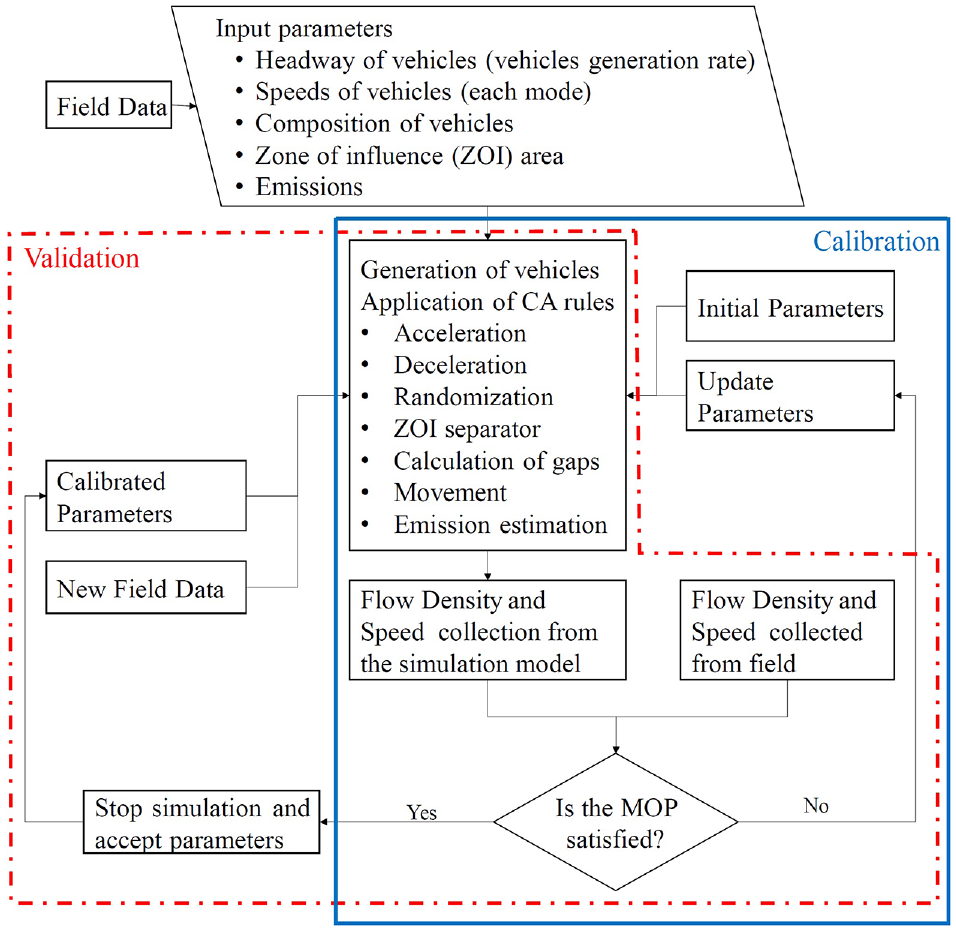
Figure 1 depicts the simulation methodology including the following steps:

1) The boundaries of the simulation model in CA play a crucial role, especially at intersections. The present model choses an open boundary over closed boundaries for several reasons, as presented in a study by Singh and Rao ( 38 , 39 ).

2) Inputs such as flow/density, type of mode, length of each approach, dimensions of vehicles, proportion of left, straight, and right vehicles, cycle length, and so forth were collected from the field and given as input to the model. These inputs were used to generate vehicles with predefined characteristics.

3) The generated vehicles calculate front, left, and right neighborhood gaps. They also calculate the gap from the road ends.

4) Vehicles change their behaviors when they are near to the intersection (based on IZOI).

5) Further, some small-size vehicles coming later seep through the gaps between other vehicles and reach near the intersection. When the signal turns green, they move in their chosen directions (left, right, or straight). If the signal is red, vehicles are forced to decelerate and stop before the intersection. Therefore, the randomization parameter was not provided when vehicles were in the IZOI.

6) When vehicles reach near the end of the intersection approach (see bold red dots marked in Figure 1) they get deleted.

7) Required data is collected while the simulation is in progress. This data can be used for calibration and validation.

Figure 1.

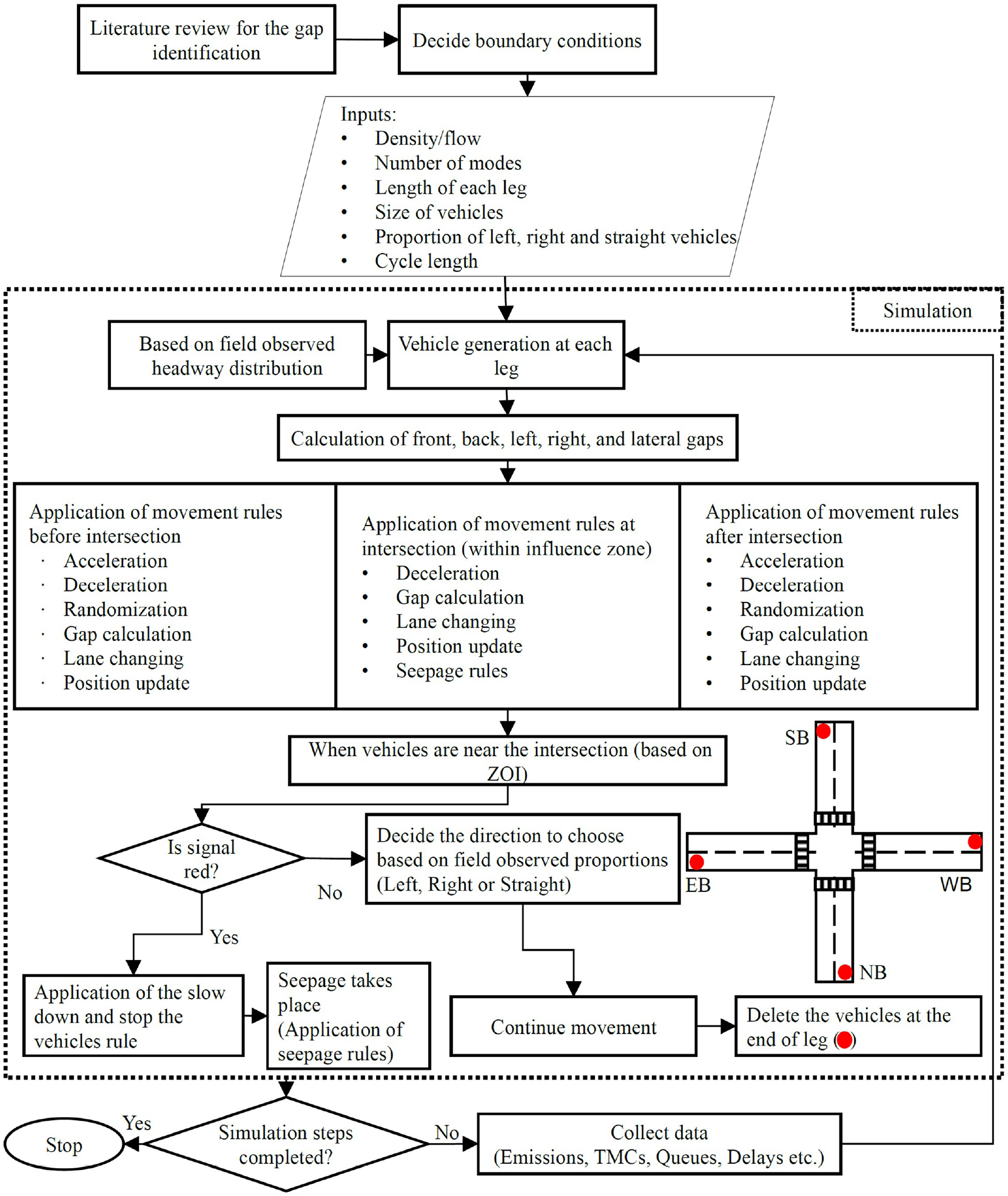
Overall simulation methodology.

Vehicle Modeling

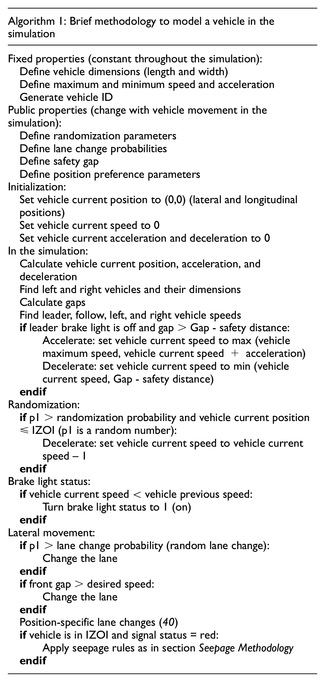
The process of vehicle modeling commences with the establishment of fixed attributes, such as the dimensions of the vehicle, its maximum and minimum speeds, accelerations, and the generation of an ID for the vehicle (Algorithm 1). In addition, various public properties that change with the advancement of simulation are defined, including parameters related to randomization, lane-change probabilities, safety gaps, and position preferences. The initial values for the vehicle’s position, speed, acceleration, and deceleration are all set to zero. During the simulation, the vehicle’s current location, acceleration, and deceleration are computed. The leader, follower, left, and right vehicle types and gaps, as well as their speeds, are identified. The acceleration or deceleration of the vehicle is dependent on the brake light status and gap of the leading vehicle. The process of randomization is implemented by decelerating when specific conditions are satisfied. The activation of the brake light occurs when the current velocity of the vehicle is lower than its preceding velocity. The determination of lateral movement is influenced by factors such as lane change probability, front gap, and position-specific lane changes, as discussed in a previous study ( 40 ). This methodology is adhered to by all vehicles. However, as a result of the small dimensions of two-wheelers, they have a tendency to develop higher levels of seepage in comparison with other modes of transportation. The parameters for each mode exhibit variations and are determined through the calibration process, as outlined in the Calibration and Validation section.

Algorithm 1: Brief methodology to model a vehicle in the simulation
Fixed properties (constant throughout the simulation): Define vehicle dimensions (length and width) Define maximum and minimum speed and acceleration Generate vehicle ID Public properties (change with vehicle movement in the simulation): Define randomization parameters Define lane change probabilities Define safety gap Define position preference parameters Initialization: Set vehicle current position to (0,0) (lateral and longitudinal positions) Set vehicle current speed to 0 Set vehicle current acceleration and deceleration to 0 In the simulation: Calculate vehicle current position, acceleration, and deceleration Find left and right vehicles and their dimensions Calculate gaps Find leader, follow, left, and right vehicle speeds if leader brake light is off and gap > Gap - safety distance: Accelerate: set vehicle current speed to max (vehicle maximum speed, vehicle current speed + acceleration) Decelerate: set vehicle current speed to min (vehicle current speed, Gap - safety distance) endif Randomization: if p1 > randomization probability and vehicle current position ≤ IZOI (p1 is a random number): Decelerate: set vehicle current speed to vehicle current speed – 1 endif Brake light status: if vehicle current speed < vehicle previous speed: Turn brake light status to 1 (on) endif Lateral movement: if p1 > lane change probability (random lane change): Change the lane endif if front gap > desired speed: Change the lane endif Position-specific lane changes ( 40 ) if vehicle is in IZOI and signal status = red: Apply seepage rules as in section Seepage Methodology endif

Algorithm 1: Brief methodology to model a vehicle in the simulation

Fixed properties (constant throughout the simulation):
Define vehicle dimensions (length and width)
Define maximum and minimum speed and acceleration
Generate vehicle ID
Public properties (change with vehicle movement in the simulation):
Define randomization parameters
Define lane change probabilities
Define safety gap
Define position preference parameters
Initialization:
Set vehicle current position to (0,0) (lateral and longitudinal positions)
Set vehicle current speed to 0
Set vehicle current acceleration and deceleration to 0
In the simulation:
Calculate vehicle current position, acceleration, and deceleration
Find left and right vehicles and their dimensions
Calculate gaps
Find leader, follow, left, and right vehicle speeds
if leader brake light is off and gap > Gap - safety distance:
Accelerate: set vehicle current speed to max (vehicle maximum speed, vehicle current speed + acceleration)
Decelerate: set vehicle current speed to min (vehicle current speed, Gap - safety distance)
endif
Randomization:
if p1 > randomization probability and vehicle current position ≤ IZOI (p1 is a random number):
Decelerate: set vehicle current speed to vehicle current speed – 1
endif
Brake light status:
if vehicle current speed < vehicle previous speed:
Turn brake light status to 1 (on)
endif
Lateral movement:
if p1 > lane change probability (random lane change):
Change the lane
endif
if front gap > desired speed:
Change the lane
endif
Position-specific lane changes ( 40 )
if vehicle is in IZOI and signal status = red:
Apply seepage rules as in section Seepage Methodology
endif

Driver Behavior and Influence Zone of Intersections (IZOI)

It was assumed that vehicles behave differently while approaching the intersection (mid-block), near the intersection, and at the intersection, after sighting the signal. Therefore, to find the influence of the intersection, the distance at which vehicles start reducing their speeds after the signal is sighted (Figure 2) was found with the help of GPS data. Subsequently, it was assumed that this is the threshold distance separating the behavior of vehicles before and at the intersection. A signalized junction with straight approaches was chosen for this study as, from a straight road, a signal can be seen from a distance. Vehicles were moved for 1 km distance to the intersection to find the threshold distance. A GPS was enabled in the vehicle to record the data. A sample size was calculated with 90% confidence interval (CI), 10% margin of error (ME), and with proportion of 0.5 which was found to be 67 per vehicle. Therefore, 100 samples were collected for each vehicle type. Subsequently, the trajectory data was extracted to analyze the speeds of the drivers after seeing the red signal. Further, a point where drivers start reducing their speeds was calculated. It was assumed that, at this location, drivers are affected by the intersection. The process was repeated for different vehicles such as cars, buses, and motorized three-wheelers (known as auto [tuk-tuk] in India). Vehicles are slow and have similar behavior in high or congested traffic; therefore, data was collected in non-peak hours. The sample size was calculated using following Equation 1 ( 41 )

n = z^{2} \frac{p (1 - p)}{M E^{2}}

(1)

where

n = the number of samples required,

z = critical value of normal distribution at some CI (say at 90%, z = 1.64), and

p = proportion of population.

Figure 2.

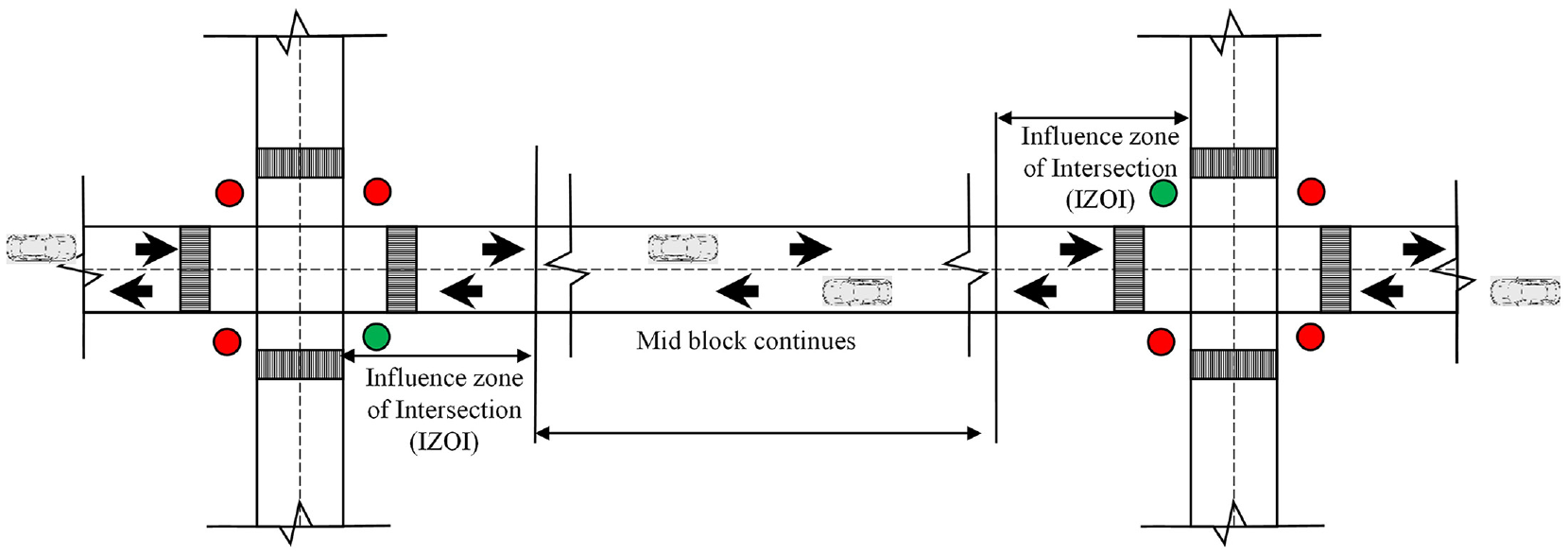
Influence zone of intersections (IZOI).

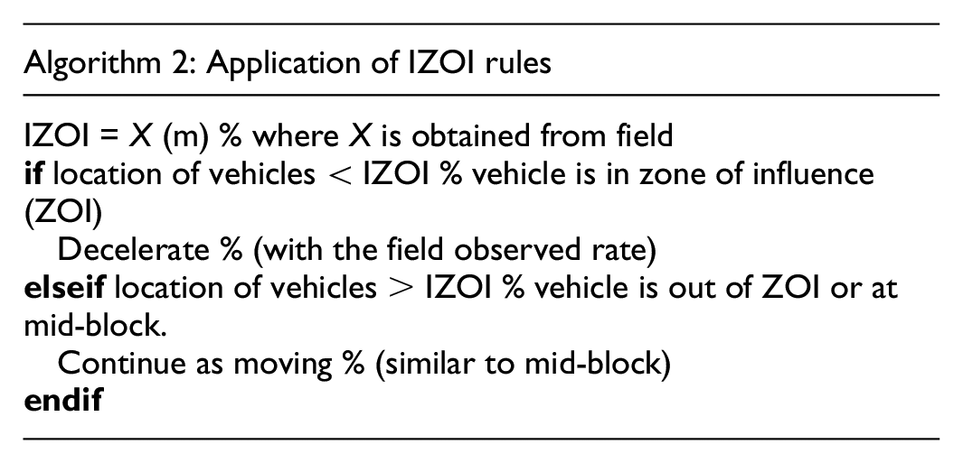
The field observations were used to model the behavioral rules for vehicle movement in addition to the traffic dynamics under various conditions at the signalized intersections. For example, it is commonly observed that vehicles reduce their speed as soon as they see a red phase at the traffic signal while approaching the intersection. If the signal is green, they would continue to move as they would in a normal mid-block location. CA rules were modified based on the IZOI; rules before the intersection, near the intersection, and after the intersection are different, as shown in Algorithm 2.

Algorithm 2: Application of IZOI rules
IZOI = X (m) % where X is obtained from field if location of vehicles < IZOI % vehicle is in zone of influence (ZOI) Decelerate % (with the field observed rate) elseif location of vehicles > IZOI % vehicle is out of ZOI or at mid-block. Continue as moving % (similar to mid-block) endif

Procedure of Trajectory Extraction from the GPS

The GPS data was recorded at 1 s frequency. The GPS was set up to start recording only when three or more satellite signals were present. Using the GPS data, distances between each point were calculated using Equation 2 ( 42 ). This was used to find the speed of vehicles at 1 s intervals. Also, the accelerations of the vehicles were calculated.

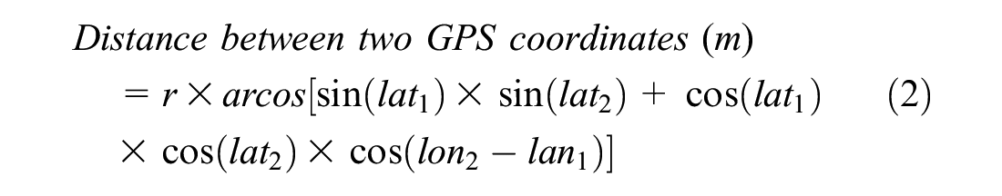
\begin{matrix} Distance between two GPS coordinates (m) \\ = r \times arcos [\sin (la t_{1}) \times \sin (la t_{2}) + \cos (la t_{1}) \\ \times \cos (la t_{2}) \times \cos (lo n_{2} - la n_{1})] \end{matrix}

(2)

where

r = radius of the Earth in meters,

lat = latitude in radians, and

lon = longitude in radians.

Figure 3, a to c , shows the deceleration behavior of motorized three-wheelers, cars, and buses. The two peaks in the data were caused by a bus stop on the data collection site (Figure 3). This influences the bus speeds, even if it was not stopping there. The distance between the bus stop and the junction was at least 500 m. It can be observed in all the figures that vehicles are affected by the intersection when they are around 200 m near the intersection. This distance was an effect of non-peak hour (no or small queue of less than 10 vehicles) traffic collected with 86 vehicles at the signalized intersection. To get a close overview of the pattern of zone of influence (ZOI), the distribution of the observed data was tested and found to be normally distributed with the following statistics.

Figure 3.

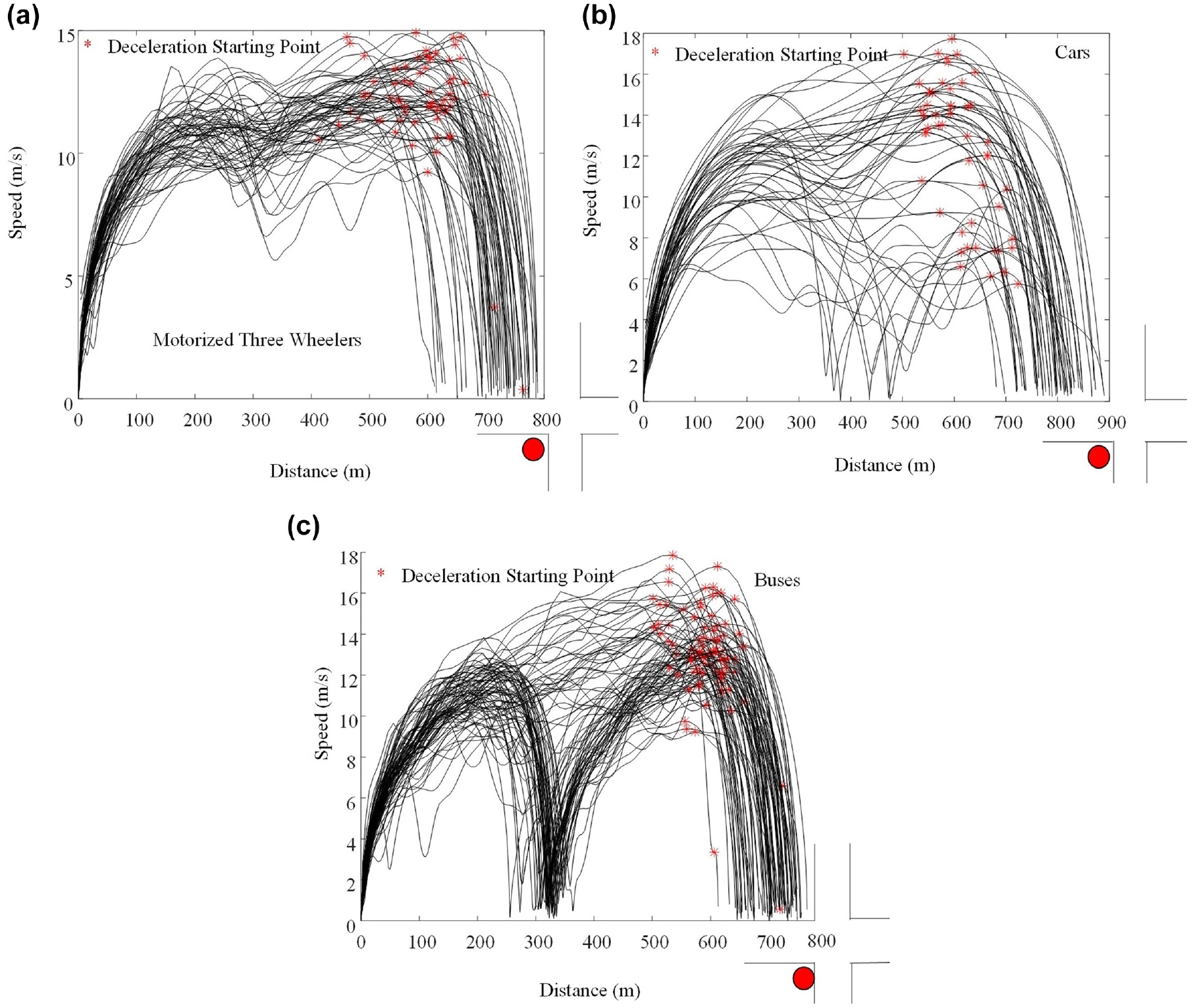
Influence of intersection on: (a) motorized three-wheelers, (b) cars, and (c) buses.

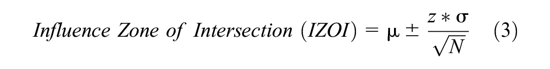
The IZOI at 95% confidence interval was found using Equation 3 and the statistics are shown in Table 1.

Influence Zone of Intersection (IZOI) = μ \pm \frac{z * σ}{\sqrt{N}}

(3)

Table 1.

Normality Test for Zone of Influence

Mode	Descriptive statistics						NDGOF		IZOI (µ±1.96*σ/√N)
Mode	N	µ	σ	Median	Min.	Max.	AD	p	Min.	Max.
Car	86	187.385	126.2821	184.108	39.1024	314.901	0.704	0.064	160.70	214.08
Bus	98	111.26	62.781	113.63	0.501875	206.41	0.213	0.848	98.83	123.69
MTW	79	141.13	74.73339	132.64	1.39209	212.64	0.578	0.129	124.65	157.61

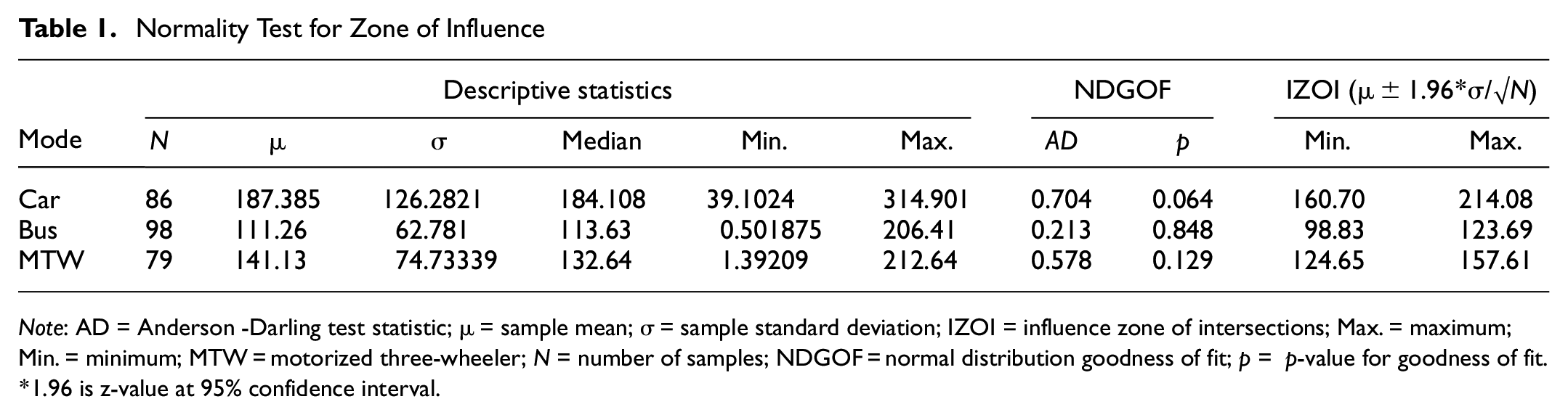
Note: AD = Anderson -Darling test statistic; µ = sample mean; σ = sample standard deviation; IZOI = influence zone of intersections; Max. = maximum; Min. = minimum; MTW = motorized three-wheeler; N = number of samples; NDGOF = normal distribution goodness of fit; p = p-value for goodness of fit.

1.96 is z-value at 95% confidence interval.

Seepage Methodology

Seepage behavior is commonly observed in the non-lane-based traffic of India and in some other South Asian countries (such as Bangladesh, Sri Lanka, and China). Figure 4, a to d , can be used to understand this phenomenon in the field. In Figure 4a, a motorized two-wheeler is trying to pass through the gaps between two cars.

Figure 4.

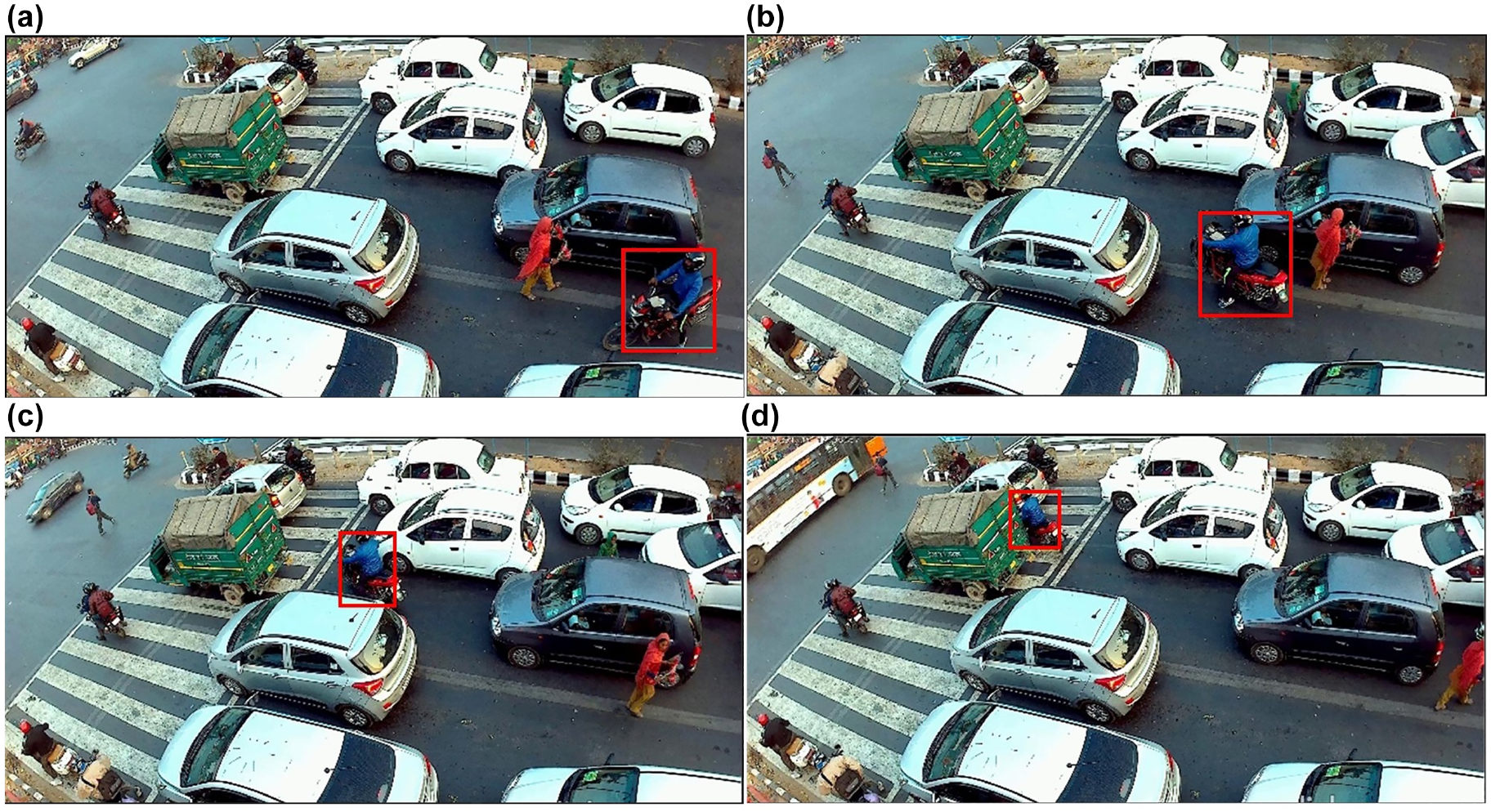
Field-observed seepage behavior: (a) Two-wheeler at a time instance (b) Two-wheelers finding gap between two cars, (c) Two-wheeler seeping through the gap between two cars, (d) Two-wheeler repeating previous steps (a)-(c) to reach to the front of intersection.

Figure 5 can be useful to understand the modeling of seepage behavior using CA. When the vehicles come to a stop as a result of a red phase of the signal (as depicted in the first and second ellipses of Figure 5), larger vehicles such as buses, trucks, and cars leave a gap (as indicated in the third ellipse of Figure 5) in front of the intersection. Motorcycle riders assess the width of a gap and proceed through it if it exceeds both their vehicle’s dimensions and the necessary safety clearance. This maneuver allows them to seep through to be near the stop-bar at the intersection, as depicted in the fourth ellipse of Figure 5. The following steps depict this process.

Figure 5.

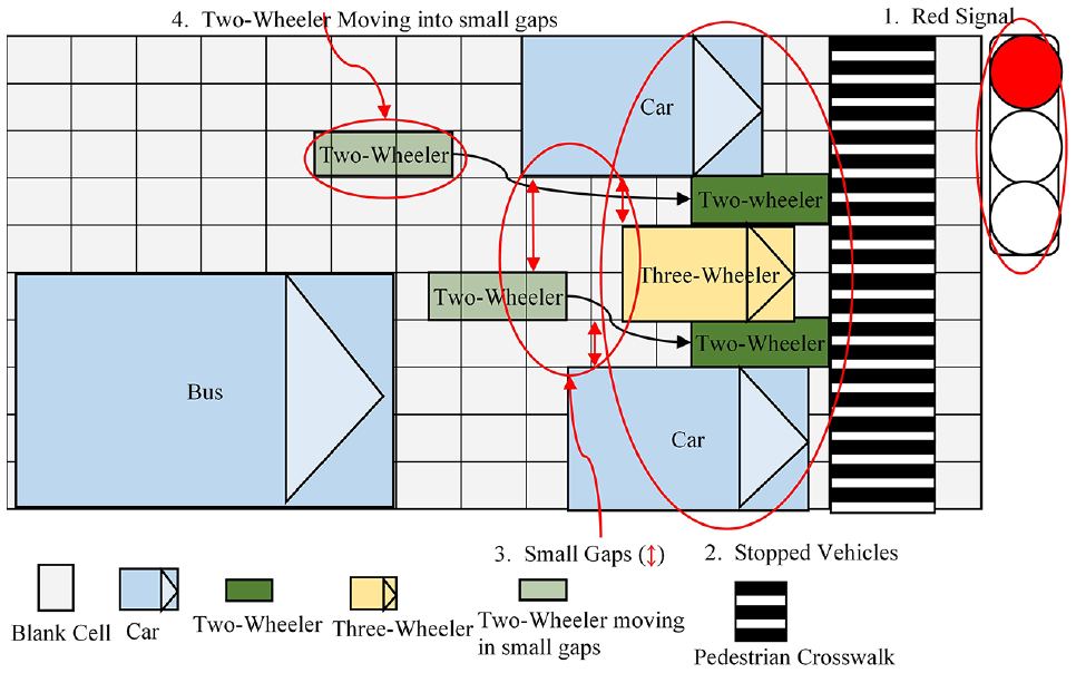
Seepage behavior modeling methodology in current cellular auromata model.

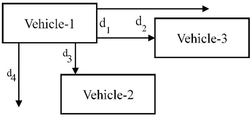
1) Vehicles are by default set to move in front. However, when they are near the intersection, their main purpose is to seep through the available gaps between vehicles and reach the beginning of the intersection. They can choose to use the available gap on any side (right, left, or straight) of vehicles to go to the front of the intersection. Lateral and longitudinal gaps are calculated as given in Equations 4 and 5, respectively. The gaps d₁, d₂, d₃, and d₄ are shown in Figure 6. In the present study, it has been considered that the vehicle will only seep if sufficient lateral and longitudinal gaps are available, otherwise it will stay at its position. If several vehicles are moving before a vehicle (such as car and truck) then the vehicle has ability to choose its leader based on a set of predefined parameters ( 40 , 43 ).

2) In each step, all the vehicles check whether they can pass through the available gap. If their size is less than the available gap, then they seep.

Figure 6.

Calculation of lateral and longitudinal gaps.

Lateral gap = min (d_{4}, d_{3})

(4)

Longitudenal gap = \min (d_{1}, d_{2})

(5)

A stepwise algorithm to calculate the spaces is given in Algorithm 3 and Figure 7 with the above steps:

Algorithm 3: Seepage behavior
Give the size of vehicle forv = 1: number of vehicles Check left side gap for vehicle (v) Check right side gap for vehicle (v) Check front gap for vehicle (v) if left side gap for vehicle (v) >size of vehicle (v) + lateral and longitudinal safe distance Seep to left elseif right side gap for vehicle (v) >size of vehicle (v) + lateral and longitudinal safe distance Seep to right elseif lateral position of 1st front vehicle − lateral position of 2nd front vehicle > size of vehicle + lateral and longitudinal safe distance Seep in-between two vehicles else Reduce speed and stop slowly endif endfor

Algorithm 3: Seepage behavior

Give the size of vehicle
forv = 1: number of vehicles
Check left side gap for vehicle (v)
Check right side gap for vehicle (v)
Check front gap for vehicle (v)
if left side gap for vehicle (v) >size of vehicle (v) + lateral and longitudinal safe distance
Seep to left
elseif right side gap for vehicle (v) >size of vehicle (v) + lateral and longitudinal safe distance
Seep to right
elseif lateral position of 1st front vehicle − lateral position of 2nd front vehicle > size of vehicle + lateral and longitudinal safe distance
Seep in-between two vehicles
else
Reduce speed and stop slowly
endif
endfor

Figure 7.

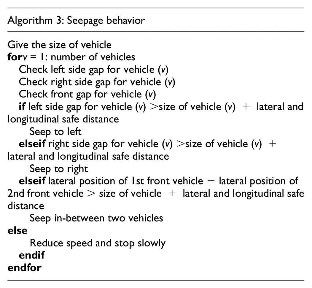
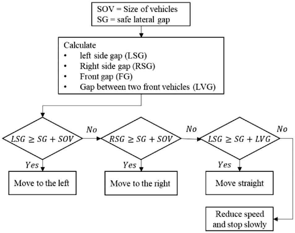
Seepage behavior modeling algorithm.

Intersection Modeling

Based on the above steps and a host of other rules, a simulation model for signalized intersections was developed to incorporate the heterogeneous non-lane-based traffic driver behavior and seepage behavior. Vehicles change their characteristics based on the IZOI. Simulation of vehicles can be understood with Figure 8. Vehicles are generated at the beginning of each approach based on a predefined field observed headway. These vehicles move based on the CA rules described above. The vehicles after crossing the junction get deleted.

Figure 8.

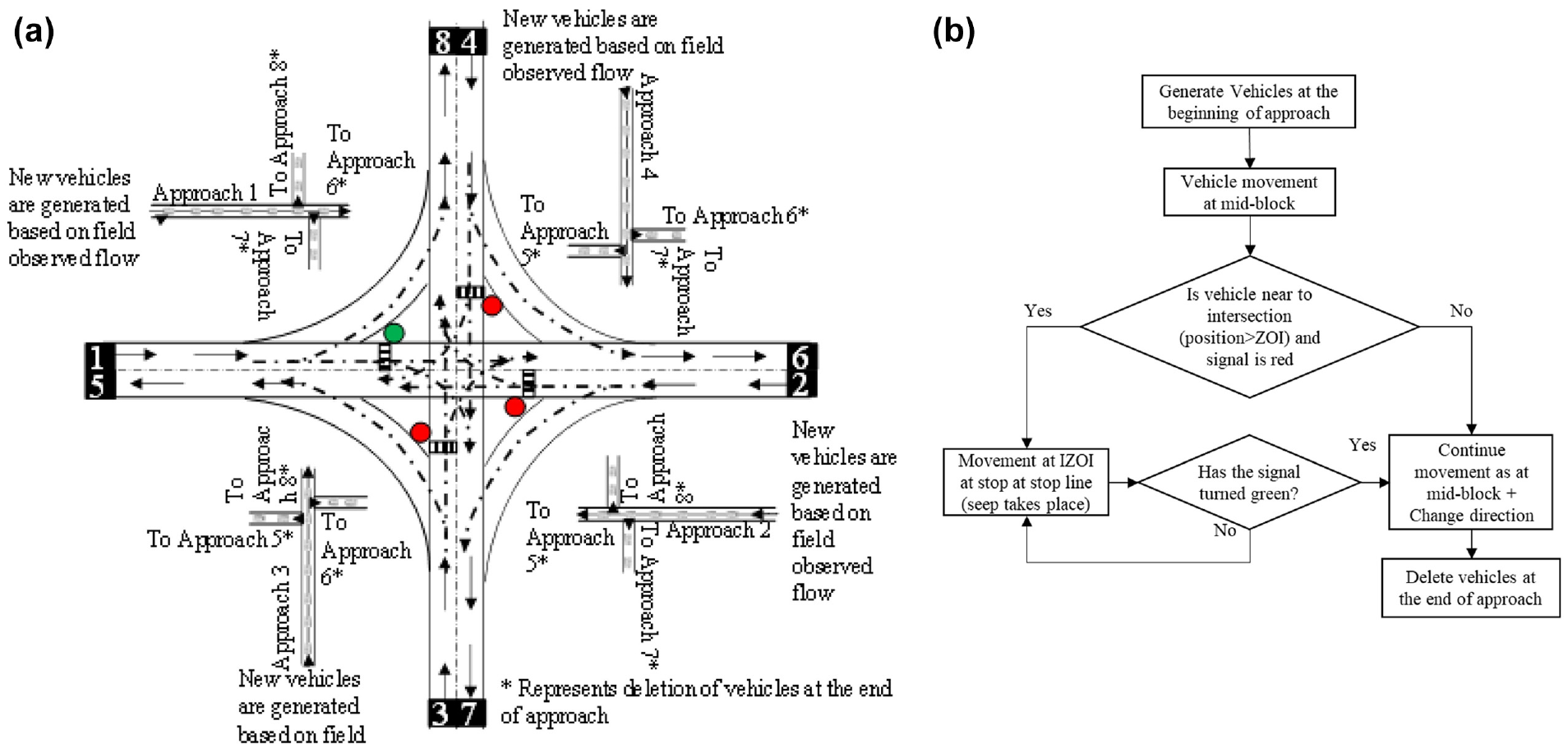
Intersection simulation methodology: (a) Plan of the intersection modelled in the study and (b) Methodology of vehicle movement in the simulation model.

Calibration and Validation Methodology

Calibration and validation are the critical steps before the simulation model can be utilized for any purpose. The inputs provided to the simulation models were a combination of microscopic (maximum speed and initial acceleration) and macroscopic (traffic flow) parameters. The model was calibrated with the help of density and flow (Equation 16), with several parameters (Table 2) including microscopic ones (acceleration). Later, it was validated macroscopically and microscopically. The macroscopic validation is well known and has been discussed in various studies, but as one of the objectives was to model the seepage behavior, it was validated microscopically in addition to macroscopic validation ( 44 , 45 ). Similar microscopic validation has been discussed in Toledo and Koutsopoulos, Punzo and Simonelli, and Wu et al. ( 46 – 48 ).

Table 2.

Calibrated Parameters

S. No.	Parameter	Two-wheeler	Three-wheeler	Car	Bus and truck
1	Length (cells)	4	6	7	25
2	Width (cells)	1	2	3	3
3	Maximum speed (cells/s)	28	22	28	22
4	Acceleration (cells/s²) speed <5.5 m/s	2	1	3	1
5	Acceleration (cells/s²) at 5.5<speed<11 m/s	3	1	2	1
6	Acceleration >11 (cells/s²)	1	1	1	1
7	p_o	0.29	0.17	0.06	0.16
8	p_dec	0.98	0.74	0.94	0.5
9	α	1.25	7.14	7.73	3
10	p_bl	0.02	0.91	0.63	0.7
11	p_lc	0.23	0.8	0.1	0.97
12	Security distance (cells)	10	2	4	3
13	Interaction headway (s)	24	7	14	10
14	β	5.31	1.35	5.73	6.13

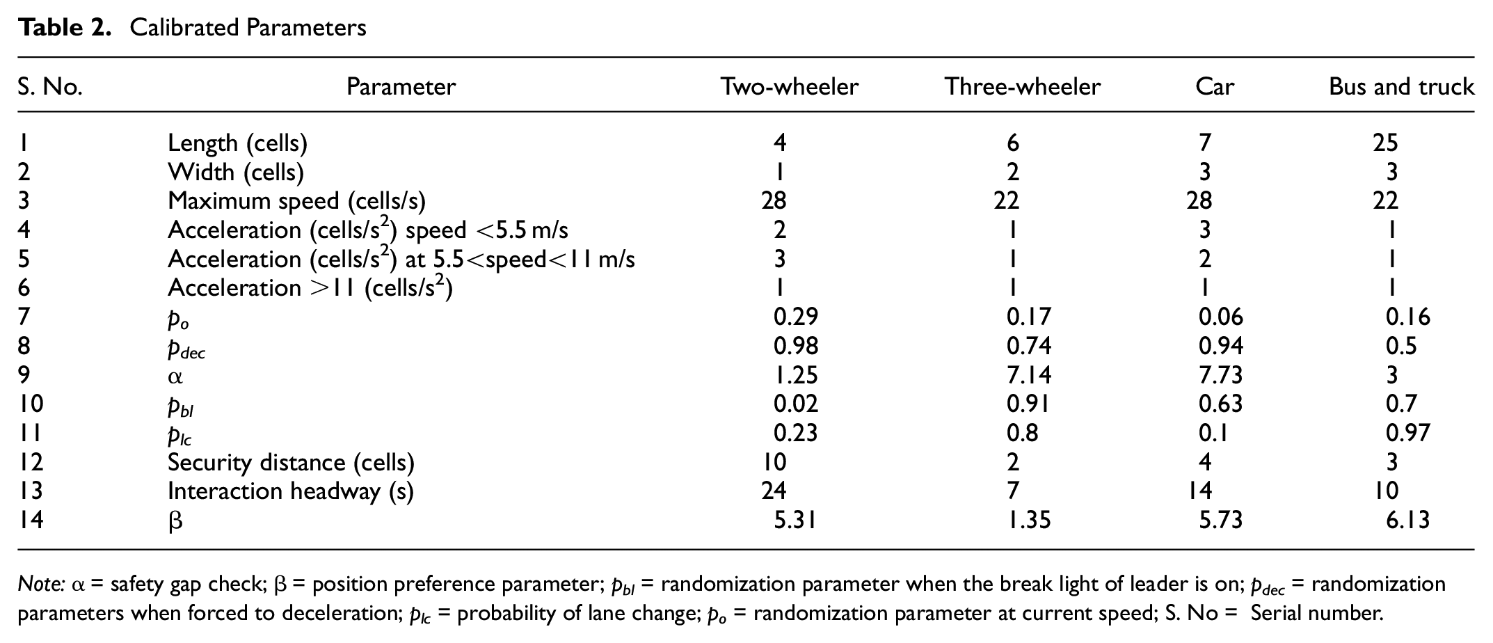
Note: α = safety gap check; β = position preference parameter; p_bl = randomization parameter when the break light of leader is on; p_dec = randomization parameters when forced to deceleration; p_lc = probability of lane change; p_o = randomization parameter at current speed; S. No = Serial number.

Flow and Density Calculation

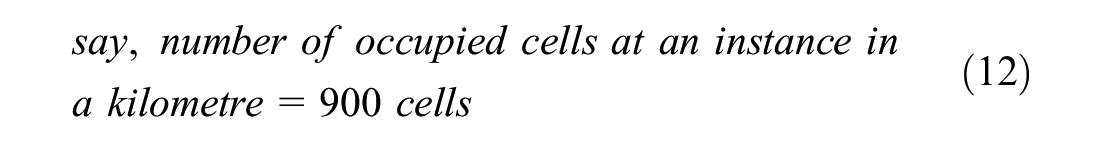
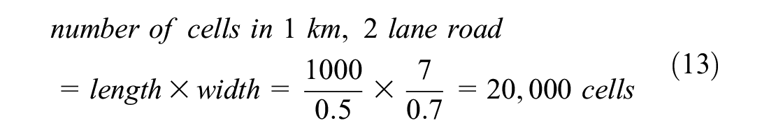
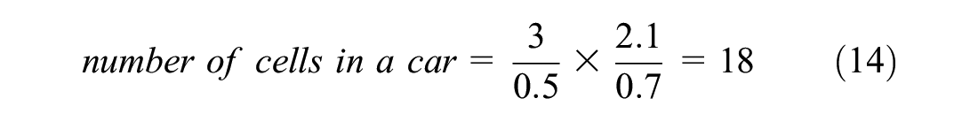
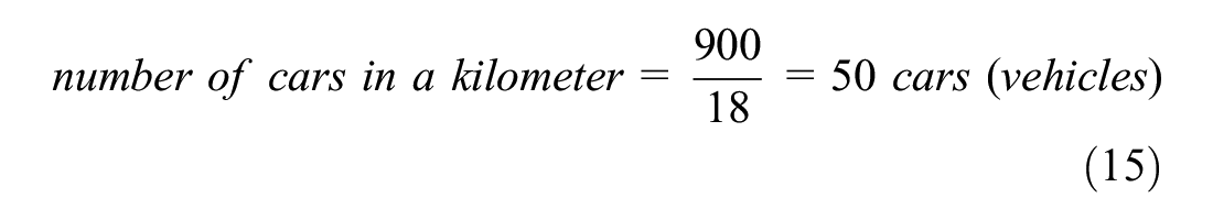
The current study simulated a non-lane-based scenario. In the present study, the number of vehicles passing a section in an hour is called traffic flow. The density was calculated as the number of vehicles per kilometer, and the flow was calculated as the number of vehicles per hour. These were calculated on the full width of the road, that is, two lanes. The road was divided into cells with a size of 0.5 m length and 0.7 m width ( 49 , 50 ). The width of the road was taken as 3.5 m based on the Indian standard ( 51 ). This means that a 1 km, two-lane road would consist of 20,000 cells (2,000 cells lengthwise and 10 cells width-wise). The dimensions of cars were taken as 2.1 m in width and 3 m in length, which would occupy an area of 18 cells (3 cells in width and 6 cells in length). The density was then calculated based on the number of occupied cells in 1 km. For example, if 900 cells are occupied at an instance, then the density would be 900 cells per 20,000 cells (1 km), which results in 50 cars per kilometer (900/18 cars per km), which results in 50 cars (900/18 vehicles here) per kilometer. The density calculation is explained with an example shown below:

Road length = 1000 m

(6)

Road width = 7 m

(7)

Cell length = 0.5 m

(8)

Cell width = 0.7 m

(9)

Vehicle length = 3 m

(10)

Vehicle width = 2.1 m

(11)

\begin{matrix} say, number of occupied cells at an instance in \\ a kilometre = 900 cells \end{matrix}

(12)

\begin{matrix} number of cells in 1 km, 2 lane road \\ = length \times width = \frac{1000}{0.5} \times \frac{7}{0.7} = 20, 000 cells \end{matrix}

(13)

number of cells in a car = \frac{3}{0.5} \times \frac{2.1}{0.7} = 18

(14)

number of cars in a kilometer = \frac{900}{18} = 50 cars (vehicles)

(15)

Calibration and Validation

The video data was collected in Delhi for 2 h per day for 3 days. This data was used to extract the traffic flow and density on the road. Another dataset for the same duration on different days was collected in Mumbai for the validation purpose of the simulation. The extraction of data was carried out through the utilization of MTraDE ( 52 ). The measure of performance (MoP) utilized to calibrate and validate the model consisted of the flow and densities of the vehicles. To calibrate the model (Equation 4), the flow data acquired from the field and simulation were minimized in their difference. Figure 9 presents a concise methodology for model calibration. The input parameters derived from the field, including headway, speed, composition, and IZOI, were provided. The study involved calibrating the parameters that are not readily observable in the field, such as acceleration, deceleration, randomization, and safe gaps, to align with the flow observed in the field. The model was calibrated and validated as follows:

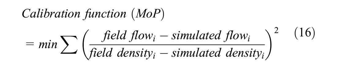
\begin{matrix} Calibration function (MoP) \\ = \min \sum {(\frac{field flo w_{i} - simulated flo w_{i}}{field densit y_{i} - simulated densit y_{i}})}^{2} \end{matrix}

(16)

where

i = the field and simulated data at 5 min intervals for 1 h.

Figure 9.

Calibration and Validation Methodology

A hybrid multi-objective optimization function combining gamultiobj and fgoalattain of the MATLAB Optimization Toolbox™ was used to optimize the parameters of the model ( 53 ). This model uses the genetic algorithm (GA) and goal attainment method simultaneously. The gamultiobj function employs a controlled and elitist GA, which is a modified version of NSGA-II ( 54 , 55 ). The gamultiobj function has the capability to automatically invoke the hybrid function fgoalattain to achieve a higher degree of precision in the solution. The function fgoalattain further solves the goal attainment problem for minimizing a multiobjective optimization problem using the inputs received from gamultiobj.

This approach was used to save on optimization time. GA optimizations are accurate, but it takes more time. Whereas goal optimization is fast, it depends on the initialization of parameters and optimizes locally. Therefore, GA is used to reach near global optimum (initialization points for goal attainment), and then a local optimum approach to goal attainment optimization is used for calibrating the parameters ( 56 ). This approach is called hybrid multi-objective optimization. There were 44 parameters for all four modes (11 each) included in the model: cars, buses, motorized two-wheelers, and motorized three-wheelers) (S. No. 4–14 in Table 2) to optimize. Further details on these parameters are given in some earlier models ( 40 , 43 ). Calibrated parameters are given in Table 2.

Macroscopic Validation

The calibrated model, having been developed, needs to be validated. Simulation runs were made to generate a new dataset. There could be several methods to check whether the data obtained from simulation represents field conditions satisfactorily (parametric: paired t-test, two-sample t-test; nonparametric: Mann-Whitney U test, among others). As the population of the sample is not known and the sample points in the simulation and field are not the same, a two-sample t-test without assuming that the variances of simulated and field data are equal was carried out to find if the means of the two data sets (field and simulated) are the same. The flow data of simulation and field should pass the normality test before doing the t-test. It was found that both sets of data follow a normal distribution. Table 3 summarizes the field and simulated traffic flow data normalities.

Table 3.

Normality Test for Field and Simulated Data

Descriptive statistics								Goodness of fit test
N	Mean	SD	Median	Minimum	Maximum	Skewness	Kurtosis	Distribution	AD	p
Field data
60	866	362.42	840	300	1830	0.46	−0.370	Normal	0.50	0.20
Simulated data
67	1793.42	281.77	1,805	1,133.92	2,506.43	−0.033	0.409	Normal	0.47	0.24

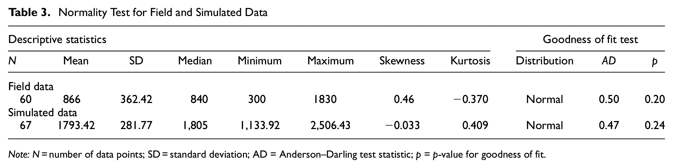
Note: N = number of data points; SD = standard deviation; AD = Anderson–Darling test statistic; p = p-value for goodness of fit.

A two-sample t-statistics of field and simulated dataset was carried out in MATLAB 2023 ( 57 ) and results are given in Table 4 with the null hypothesis as “the mean of both the samples is equal.”

Table 4.

Two-Sample t-Test for Field and Simulated Data

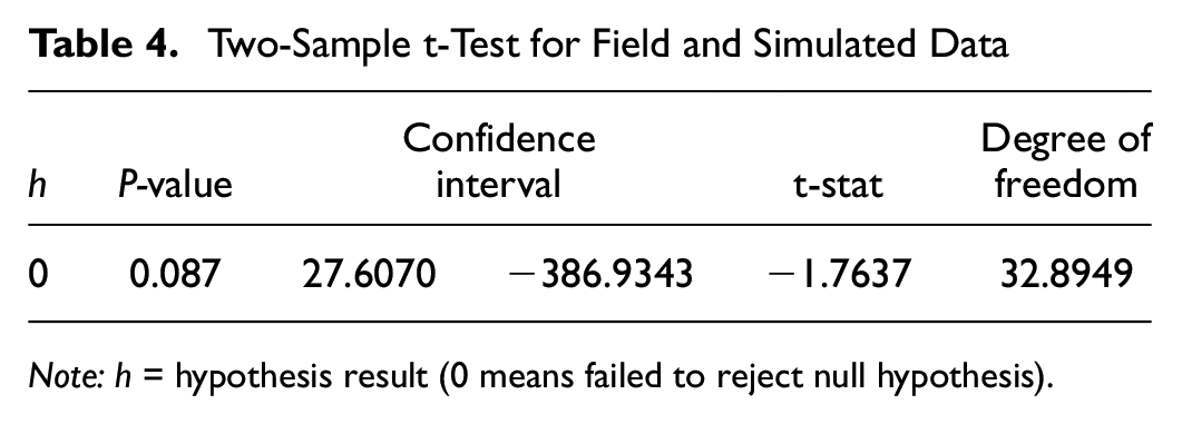
h	P-value	Confidence interval		t-stat	Degree of freedom
0	0.087	27.6070	−386.9343	−1.7637	32.8949

Note: h = hypothesis result (0 means failed to reject null hypothesis).

Figure 10a shows the q-k curves after the calibration and validation. The simulated and field data are similar to each other. The field data was observed in the free flow conditions, therefore the congested part of the field data is not visible, whereas it can be seen in the simulated part.

Figure 10.

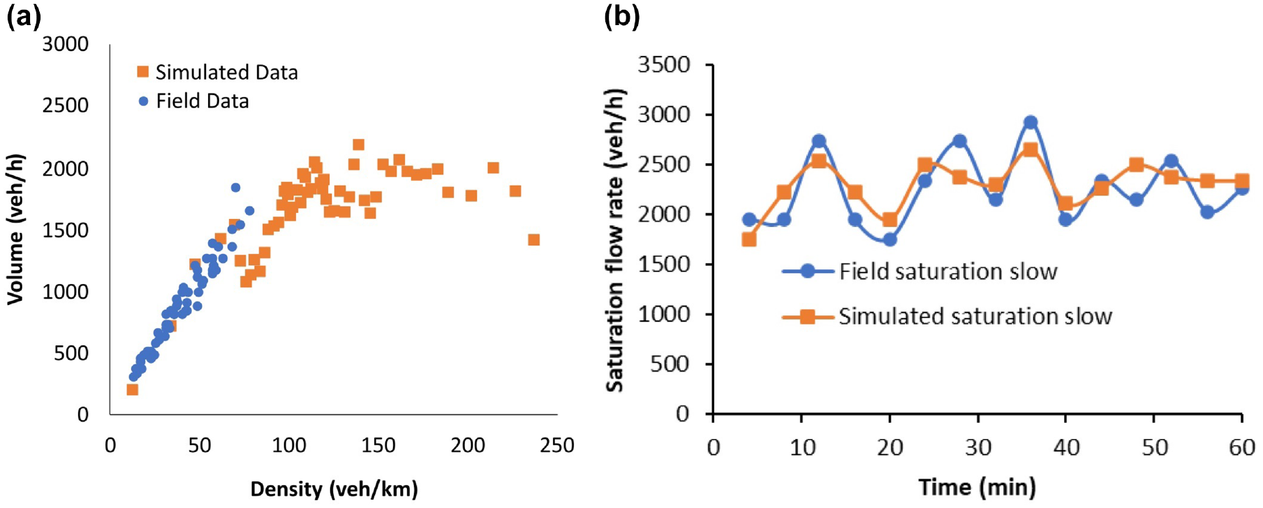
Simulated and field data comparison: (a) Comparison of simulated and field volume-density data, and (b) Comparison of simulated and field traffic flow rate.

Figure 10b specifically compares the simulated and observed saturation flow rates. The similarity between the simulated and field-measured saturation flow rates provides further evidence supporting the validity of the simulation model.

The counts obtained from the simulation model and field at 4 min intervals were compared to initially validate the simulation model. Further, field and simulation observed vehicle speed, headway, and trajectories were compared. Lastly, FDs of the simulation results were drawn and compared with theoretical FDs. The results are shown in the subsequent sections.

The visual validation of traffic flows generated from the simulation model and observed from the field can be seen from the following Figure 11. It shows that the number of vehicles generated from simulation model are comparable to the observed flow. A regression line with slope coefficient near to one confirms the close estimation of observed flows.

Figure 11.

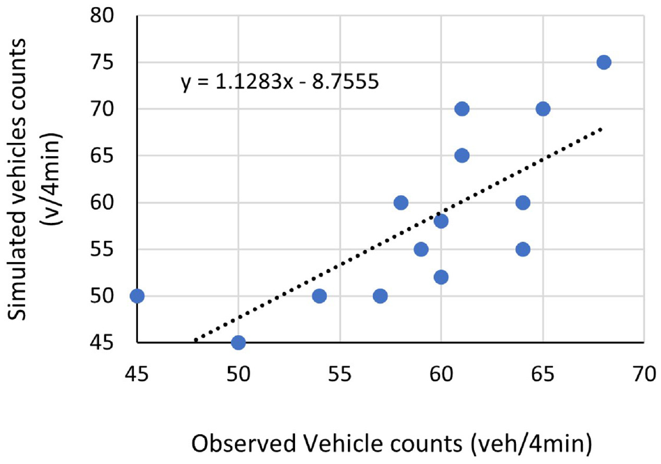
Indicative validation results.

Microscopic Validations

Figures 12 –14 depict a comparison between the trajectories, speeds, and headways obtained from both simulation and field data. The presented data indicates that the simulation model adequately reflects the observed data. Figure 12 displays a comparison of headways. The distance between the leading and trailing vehicles gradually increases until both the drivers perceive a sense of safety. This phenomenon is discernible from both simulated and empirical data. The observed incongruity between the graphs presented in Figure 12 may be attributed to a temporary phenomenon of vehicular clustering, as simulated in the model.

Figure 12.

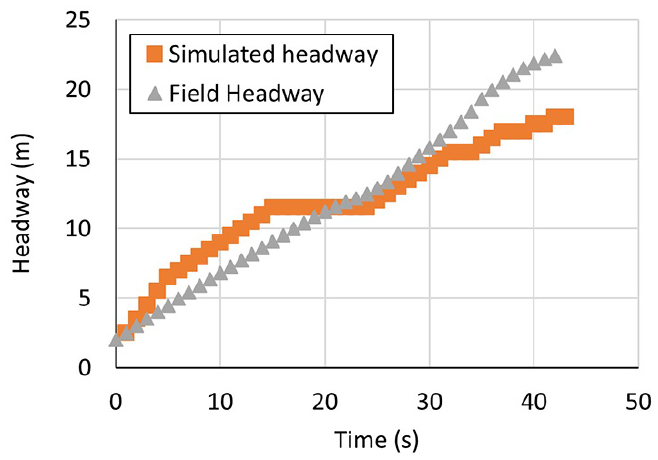
Field and simulation headways comparison.

Figure 13.

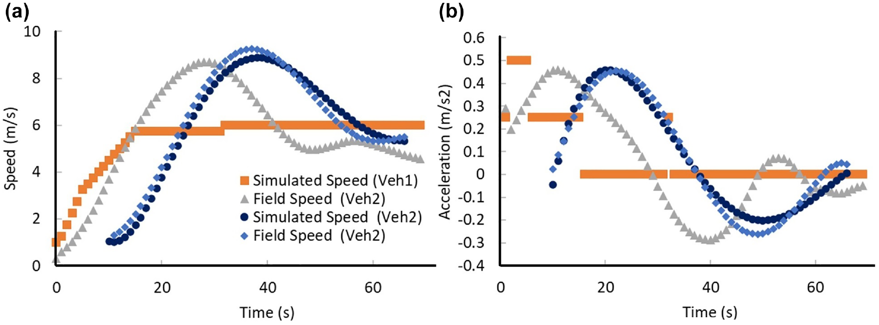
Field and simulation speeds and acceleration comparison: (a) Comparison of simulated and field speed data, and (b) Comparison of simulated and field acceleration data.

Figure 14.

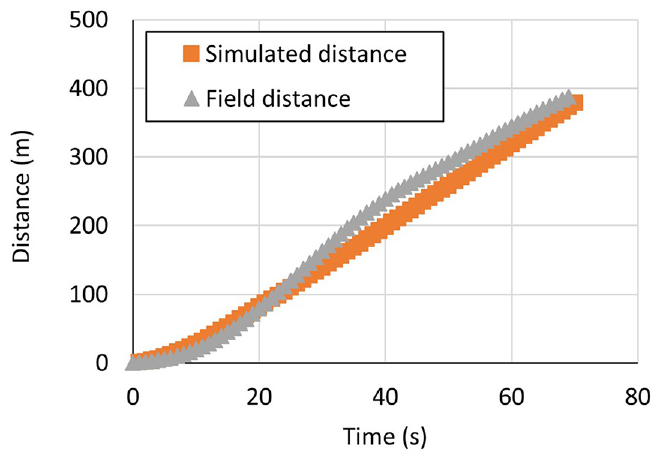
Field and simulation trajectories comparison.

The graphical representation of speed and acceleration over time for both simulated and field data, as depicted in Figure 13, reveals that the speed of vehicles in the field exhibits greater variability in comparison with the simulated data. This observation may be because the simulation model places a maximum speed limit on each vehicle, which none of the vehicles exceed. In certain field driving contexts, it is possible that some drivers may not adhere to predetermined behavioral norms and instead opt to drive at speeds that are more convenient and appropriate for them (i.e., over-speeding) given the surrounding traffic conditions. This behavior can be observed in some existing studies as well ( 58 ). In general, it can be observed from Figure 13 that the simulated and observed speeds and acceleration are in coherence after a certain period of simulation time.

The trajectory plot (distance [x] − time [t]) of simulated and observed data is shown in Figure 14. It can be observed that both simulated and observed data follow a similar trajectory.

The present study uses the following measures of performances to further validate the simulation model.

The following statistics were used for the validation of the model.

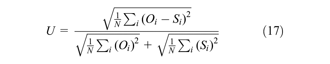
1) Theil’s U-coefficient, with its bias (U_M), variance (U_S), and covariance (U_C) components. Subsequent Equations 16 to 20 were used to calculate these ( 47 ).

U = \frac{\sqrt{\frac{1}{N} \sum_{i} {(O_{i} - S_{i})}^{2}}}{\sqrt{\frac{1}{N} \sum_{i} {(O_{i})}^{2}} + \sqrt{\frac{1}{N} \sum_{i} {(S_{i})}^{2}}}

(17)

U_{M} = \frac{{(μ_{s} - μ_{o})}^{2}}{\frac{1}{N} \sum_{i} {(O_{i} - S_{i})}^{2} ρ}

(18)

U_{S} = \frac{{(σ_{s} - σ_{o})}^{2}}{\frac{1}{N} \sum_{i} {(O_{i} - S_{i})}^{2}}

(19)

U_{C} = \frac{2 (1 - ρ) σ_{s} σ_{o}}{\frac{1}{N} \sum_{i} {(O_{i} - S_{i})}^{2}}

(20)

2) Root mean square error (RMSE) ( 59 )

RMSE = \sqrt{\frac{1}{N} \sum_{i} {(O_{i} - S_{i})}^{2}}

(21)

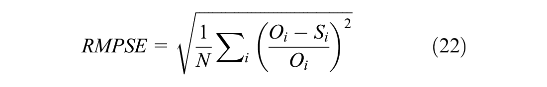
3) Root mean square percentage error (RMSPE) ( 59 )

RMPSE = \sqrt{\frac{1}{N} \sum_{i} {(\frac{O_{i} - S_{i}}{O_{i}})}^{2}}

(22)

4) The GEH statistic: a statistical technique used in traffic engineering, forecasting, and modeling to compare sets of traffic volumes ( 60 ).

GEH = \sqrt{\frac{{(V_{S} - V_{O})}^{2}}{(V_{S} + V_{O}) / 2}}

(23)

where

o = observed data,

s = simulated data,

V = volume of simulated (V_S) and field data (V_O), and

N = total number of samples.

The Theil’s U-coefficient, with its bias, variance, and covariance components, is shown in Figure 15a. It is known that a smaller Theil’s coefficient shows a better estimate of observed data. It can be seen from Figure 15a that the Theil’s coefficient is less than 20% for simulated data of trajectories, speed, and headways. Moreover, its bias, variance, and covariance terms are also less than 1. The bias proportion of Theil’s coefficient (U_M) represents the systematic error. Its variance component tries to explain the variability in the observed and simulated data. It is considered good if these values—bias (U_M) and variance (U_S)—are closer to 0. The covariance component of Theil’s coefficient (U_C) represents the remaining error (other than bias and variance). It is considered good if this component is near to 1. This indicates that the simulation model estimates closely match the observed values.

Figure 15.

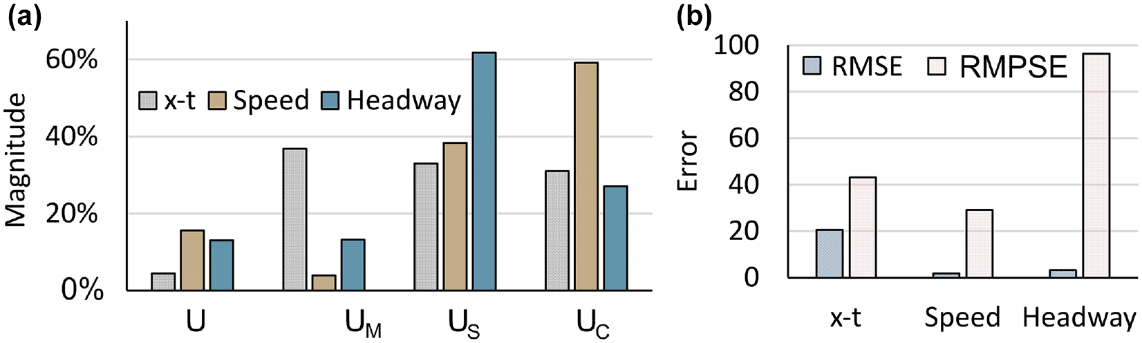
Error and Theil coefficient for trajectories (x-t), speeds and headway: (a) Theil's coefficients comparison for trajectories, speeds, and headways and (b) Observed errors for trajectories, speeds, and headways.

Further, Figure 15b shows the RMSE and RMSPE. These errors show the deviation of the simulated and observed data. These values are also very much lower and this confirms that the simulation model realistically represents the observed values.

Finally, the GEH statistic was calculated to test the validity of the model. As per the Federal Highway Administration (FHWA) guidelines, the GEH values less than 5 are considered to be a good fit for estimated and observed volumes ( 60 ). The GEH statistic calculated for the current simulation were found to be 4.01, which validates the close representation of observed data by the simulation model. Therefore, the simulation model developed in the present study is validated and it represents the observed data satisfactorily.

Results and Discussion

This section discusses the FD and simulation model results. Further, it compares the delay results with the existing manuals to demonstrate the simulation model’s applications. Results such as FDs, delays and a graphical representation of seepage were calculated and measured in the field and compared with the simulation model.

Fundamental Diagrams (FDs)

Simulations were carried out for individual transportation modes (one mode at a time) as well as mixed-traffic conditions. The resulting FDs are shown in Figure 16. The diagram in Figure 16 displays the presence of mixed-traffic flow, as indicated by the yellow (diamond shaped) and blue (left facing triangle) points. The comparable capacity of the data can be observed. This finding serves as evidence supporting the accuracy and reliability of the simulation model. Further, Figure 16, a and b , shows the simulated FDs at the intersections. It can be observed in the FDs that the order of the capacity and density is from small vehicles to large vehicles, which means high capacity and density for small vehicles and low capacity and density for large vehicles. These are similar to the curves observed theoretically in the study done in Delhi by Gaddam and Rao ( 61 ).

Figure 16.

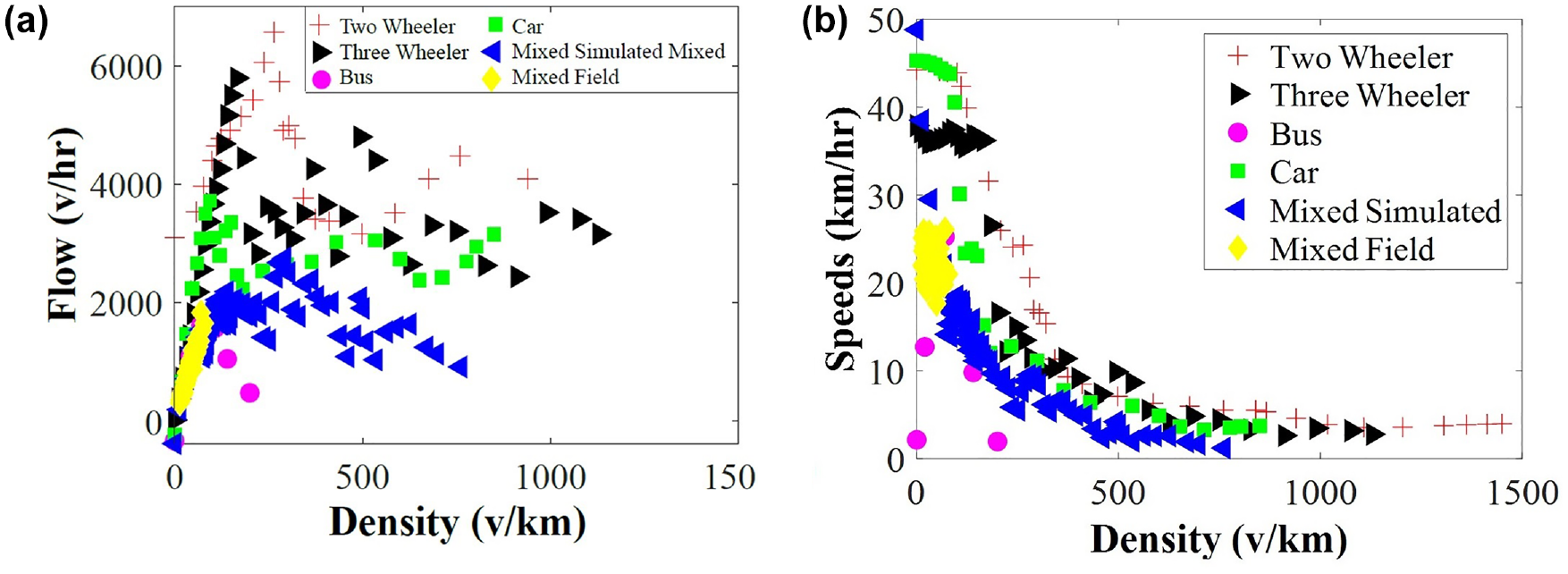
Simulated flow-density curve: (a) Comparison of simulated and field volume-density data for various traffic compositions and (b) Comparison of simulated and field speed-density data for various traffic compositions.

Delays

The calculation of delays used manuals from different nations, including China, India, and the U.S., among others. For the comparison, the delays from the field were also collected. It has been noted that the delays calculated using different manuals (such as in Table 5) do not directly take the seepage into account. Nevertheless, these models have been designed with various adjustment factors to compute the overall estimation of anticipated delays. Certain highway capacity manuals incorporate the proportion of different modes of transport when determining the extent of delays, which could be a balancing factor for the possibility of seepage ( 62 , 63 ). Seepage is an inevitable occurrence in India (or similar traffic behavior settings in South Asia, and Far East regions), and it is recommended to estimate delays using the respective highway capacity manual (such as the Highway Capacity Study, Indonesian Highway Capacity Manual, and Elefteriadou) to obtain a reasonable representation of the actual delay ( 62 – 64 ). This result also corroborates the field evidence that the delay formulas are often overestimates of the actual delays incurred in the heterogeneous traffic environment (Figure 17). Table 5 lists the various factors that have been taken into account when calculating delays using various capacity manuals.

Table 5.

Delays with Parameters Used

Parameter		Delay
IHCM (1993) ( 63 )
Cycle time	130
Traffic flow for approach (q_v and q_j)	2,166
Green time	30
PCE_LV	1
PCE_HV	1.5
PCE_MC	0.5
Fraction of LV	0.68
Fraction of HV	0.05
Fraction of MC	0.27
PCU factor f_pcu	0.89
Green ratio (g_r)	0.231
Cycle time (c)	130	D_j = 40.65*
Degree of saturation (ds)	0.643
Q_p = q_vp*	1,927.74
Capacity	2,996.63
Base capacity value (c₀)	3,400
Entry width correction factor (f_w)	1.09
Major road median correction factor (f_m)	1
City size correction factor (fcs)	0.94
Road environment type and side friction correction factor (f_rf)	1
Left-turning % correction factor (f_lt)	1.1
Right-turning % correction factor (f_rt)	0.92
Split correction factor (f_sp)	0.85
CHCM (1999) ( 62 )
Proportion of stopped vehicles in approach (P_sv)	0.8
Proportion of turning vehicles in approach (P_t)	0.35
Green ratio (GR)	0.23
Degree of saturation (DS)	0.89
Capacity (C)	2,221.44
Cycle time (c)	130
Number of PCU remained from previous green phase (NQ₁)	0
Saturation flow	2,598
Green time	30
Number of lanes	2	DG_j = 3.62*DT_j = 48.092*D_j = 51.716*
PCE_LV	1
PCE_HV	1.5
PCE_MC	0.5
Fraction of LV	0.68
Fraction of HV	0.05
Fraction of MC	0.27
Left-turn vehicle ratio (F_LT)	0.99
Right-turn vehicle ratio (F_RT)	1.06
Minor road ratio (F_MI)	1.2
Side friction (F_SF)	0.93
Base capacity (C₀)	1900
PCU factor (F_PCU)	0.89
Flow (Q_veh)	2166
Total actual flow (Q_PCU)	1,927.74
Degree of separation (0 for no bicycle)	0
Road width (W_EFF)	7
CaHCM (2008) ( 65 )
Adjustment factor for the effect of the quality of progression, with (k_f)*	0.99	d₁ = 40.557d₂ = 0.536d = 40.86*
Proportion of vehicles arriving during the green interval (q_gr/q)*	0.24
Average number of arrivals during green interval (q_gr)	51
Average number of arrivals per cycle (m)	217
Supplemental adjustment factor for platoon arrival time from (f_p)	1
Cycle time (c)	130
Effective green time (s) (g_e)	30
Degree of saturation (max = 1) (x₁)*	0.224
Saturation flow rate *	4,200
Capacity (C)*	969.23
Evaluation time (min) (t_e)	60
Effective width of road	7
HCM (2016) ( 64 )
Cycle time (C)	130
Volume-to-capacity ratio (X) *	0.95
Demand flow rate (vph) (v)	2,166
Capacity (vph) (c) *	2,276.3
Adjusted saturation flow rate (vphpl) (s)	4,932.1
Number of lanes in lane group (In) (N)	2
Base saturation flow rate 1,900 (pcphpl) (s₀)	1,900
Adjustment factor for lane width (f_w)	1.04
Adjustment factor for heavy vehicles in traffic stream, (f_hv)	0.96
Adjustment factor for approach grade (f_g)	1
Adjustment factor for existence of a parking lane and parking activity adjacent to lane group (f_p)	1
Adjustment factor for blocking effect of local buses that stop within intersection area (f_bb) *	1	d₁ = 49.28d₂ = 10.48d = 59.76*
Adjustment factor for area type (f_a) *	0.9
Adjustment factor for lane utilization (f_LU)	1
Adjustment factor for left-turn vehicle presence in a lane group (f_LT) *	0.99
Adjustment factor for right-turn vehicle presence in a lane group (f_RT) *	0.97
Pedestrian adjustment factor for left-turn groups (f_LPB)	1
Pedestrian-bicycle adjustment factor for right-turn groups (f_RPB)	1
Presence of work zones (f_wz) *	0.92
Number of parking movements per hour into and out of parking spaces (N_m)	0
Parking factor applied only when parking is present (P)	0
Through car equivalent for right turns (E_R)	1.18
Sum width of all open lanes (a_w)	10
Sum of left and through lanes open during work zone operation (n_wz)	0
Sum of left and through lanes open during normal operation (n₀)	2
Adjustment factor for approach width (f_wid)*	0.99
Adjustment factor for reducing lanes during existence of work zone (f_reduce)*	1.09
Indo-HCM (2017) ( 66 )
Volume (number) (V)	2,166	d₁ = 45.93d₂ = 1.75d₃ = 0.00d = 47.68
Total lost time per cycle (L)	2
Overall cycle time (CY_Time)	130
Degree of saturation (X)	0.704
Capacity of the candidate signalized intersection (in PCU/h) (C_SI)	0.704	2,483.453
Analysis period (h) (T)	1
Effective green period (g)	30
Initial queue delay (Q_b)	0
Duration of demand met (t)	0
Demand parameter (u)	0
Saturation flow (S_fi)	5,283.315
Volume (PCU)	1,717.638
Unit base saturation flow rate (in PCU/h/m) (USF₀)	714.058
Width of the road (w)	7
Adjustment factor for bus blockage because of curbside bus stop (fbb)	1
Adjustment factor for blockage of through vehicles by standing right turning vehicles (fbr)	1
Adjustment factor for the initial surge of vehicles because of approach flare and anticipation effect (f_is)	1.057

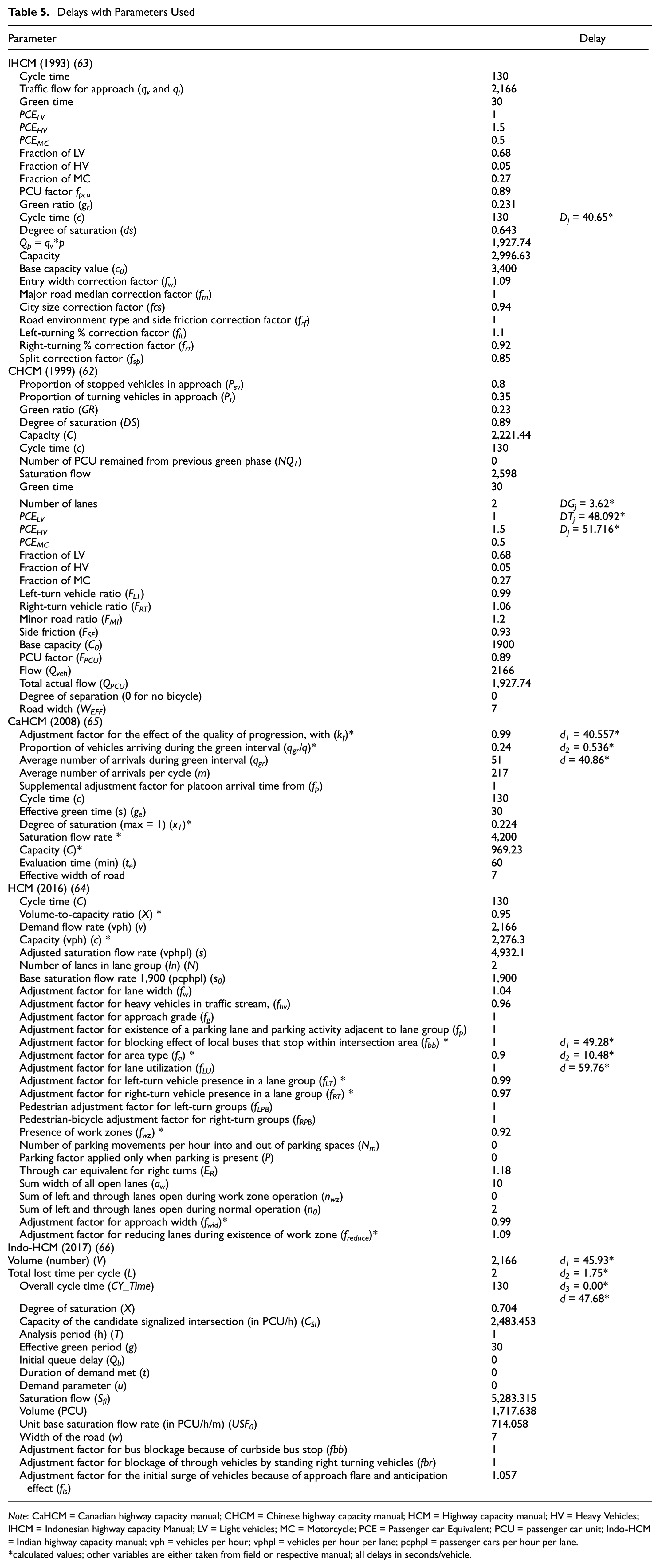
Note: CaHCM = Canadian highway capacity manual; CHCM = Chinese highway capacity manual; HCM = Highway capacity manual; HV = Heavy Vehicles; IHCM = Indonesian highway capacity Manual; LV = Light vehicles; MC = Motorcycle; PCE = Passenger car Equivalent; PCU = passenger car unit; Indo-HCM = Indian highway capacity manual; vph = vehicles per hour; vphpl = vehicles per hour per lane; pcphpl = passenger cars per hour per lane.

calculated values; other variables are either taken from field or respective manual; all delays in seconds/vehicle.

Figure 17.

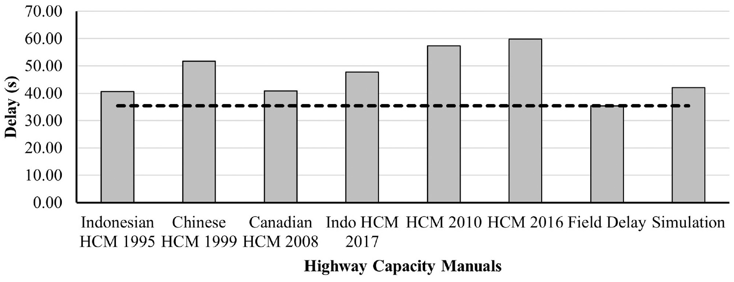
Comparison of delay from different manuals, field, and simulation.

The delays calculated from different manuals are shown in Table 5. The factors calculated as per the manuals and default and field values of the parameters used are also shown in Table 5. Delays obtained from the Indonesian and Canadian manuals are close to each other compared with other delays (40 s/veh). The delays estimated from Highway Capacity Manual (HCM) 2016 were comparatively higher than field but close to the delay from HCM 2010 (57.35 s/veh) ( 64 , 67 ). Delays obtained from several manuals are close to each other because most of these are based on Webster and Cobbe ( 68 ) formula and they consider uniform and incremental or overflow delay. There are some parts of delay considered by a few manuals, for example, only Indo HCM considers the initial queue delay, HCM 2010 considers this, and HCM 2016 does not include it anymore ( 66 ). Similarly, delays caused by the work zone affect is considered by HCM 2016. Figure 17 shows the comparison of delays obtained from different manuals’ field and simulation models. It can be observed that the simulation model delay is closer to the field delays.

Seepage

A visual presentation that illustrates the seepage dynamics in the field can be observed through a video recorded in a non-lane-based scenario at an intersection in India ( 69 ). The trajectories of vehicles under two different conditions—with and without seepage—are depicted in Figure 18. The absence of seepage (as depicted in Figure 18a from simulation) results in the trajectories being linear, forming a sequence of lines that indicate the queue formation as the vehicles stand still one after the other at the red signal of the intersection. In situations where vehicles seep, their trajectories exhibit distinct variations, and a more irregular pattern can be observed. Evidently, the motorcycles traverse the intersection despite arriving subsequent to the other vehicles. This phenomenon is also observable in the simulation and field (Figure 18, b and c , respectively). To avoid a crowded graph, Figure 18 represents a subset (zoomed version) of the various data points generated through simulation.

Figure 18.

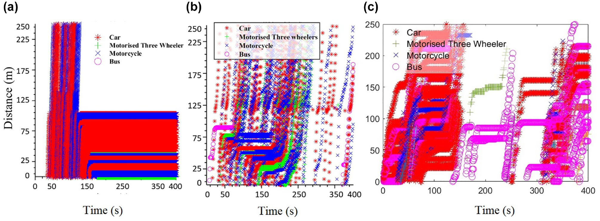
Different seepage scenarios: (a) non-seepage, simulation, (b) seepage, simulation, and (c) seepage, field.

An average of five simulated motorized two-wheeler trajectories were used to compare the simulated and field trajectory. Previous studies have fitted a regression model to compare the coefficients of field and simulated trajectories ( 47 , 70 , 71 ). However, in the present study, the Mann-Whitney U test was used to compare the trajectories observed in the field and simulation. The p-value of the test (0.96 > 0.05) directs toward failing to reject the null hypothesis. Therefore, the mean of the data observed in the field and simulation is similar. The aspect of validation visually is also discussed by other researchers ( 72 ).

Conclusions

The current model has the capability to simulate a diverse range of intersections and mid-block scenarios featuring heterogeneous traffic flow without dedicated lanes. The model incorporates supplementary attributes, namely the interaction among vehicles (seepage) and with signals. The model incorporates seepage behavior by utilizing inter-vehicle gaps, which are more realistic ( 73 ). The conformity of traffic volume pattern derived from simulation models with the field data in Delhi has been corroborated by other studies ( 61 ).

The calibration of the model was facilitated through the utilization of traffic volume and density. Moreover, the validity of the model was assessed using various performance metrics. Theil’s coefficient, computed from the observed and simulated data, was determined to be below 20%. This indicates that the simulation model adequately reflects the observed values. In addition, other statistical measures, such as RMSE and RMSPE, were found to be within acceptable thresholds (except for headways). The statistical analysis of GEH indicates that the precision of the simulation model is below 5%. This outcome aligns with the findings of the FHWA report, which suggests that such a measure is indicative of reliable simulation data ( 60 ). Therefore, the model effectively replicated the observed data and can be utilized for subsequent analyses pertaining to the estimation and optimization of delay, queue, and signal time.

The simulation models yielded a delay of 42.06 s/veh, as evidenced by Figure 17 which indicates a close correspondence between the delay obtained from the simulation model and the delays observed in the field. This particular model has the potential to effectively replicate traffic patterns in a realistic manner, while also enabling the computation of cycle times, delays, and the related metrics. The simulation can be augmented with additional emissions regulations to acquire data on vehicular emissions.

Limitations

This study does not come without limitations. The resolution of GPS was restricted to 1 s because of instrument limitations; the model could potentially be improved with the use of a GPS with higher resolution. Further, the present study utilized the mean of observed IZOI locations where deceleration was initiated following the visual detection of the red traffic signal at the intersection as a strategy for reducing vehicular speed. The behavior in question could logically be represented by a distribution that has been observed in the field.

Footnotes

Author Contributions

The authors confirm contribution to the paper as follows: study conception and design: M. Singh, K. Rao; data collection: M. Singh; analysis and interpretation of results: M. Singh; draft manuscript preparation: M. Singh, K. Rao. All authors reviewed the results and approved the final version of the manuscript.

Declaration of Conflicting Interests

The author(s) declared no potential conflicts of interest with respect to the research, authorship, and/or publication of this article.

Funding

The author(s) received no financial support for the research, authorship, and/or publication of this article.

ORCID iD

Mohit Kumar Singh

Data Accessibility Statement

Some or all data, models, or code that support the findings of this study are available from the corresponding author on reasonable request.

References

Kakooza

Luboobi

L. S.

Mugisha

J. Y. T.

Modeling Traffic Flow and Management at Un-Signalized, Signalized and Roundabout Road Intersections. Journal of Mathematics and Statistics, Vol. 1, No. 3, 2005, pp. 194–202. https://doi.org/10.3844/jmssp.2005.194.202.

Pandey

Ramachandra Rao

Mohan

A Review of Cellular Automata Model for Heterogeneous Traffic Conditions. In Traffic and Granular Flow ’13 ( Chraibi

Boltes

Schadschneider

Seyfried

, eds.), Springer International Publishing, Cham, Switzerland, pp. 471–478.

MoRTH. Road Accidents in India - 2015 (Ministry of Road Transport and Highways). MoRTH, New Delhi, India, 2016.

Dong

Zhang

Dai

Simulation on Vehicle Emission by the Brake-Light Cellular Automata Model. In Cellular Automata ( S.

Bandini

Manzoni

Umeo

Vizzari

, eds.), Lecture Notes in Computer Science (including subseries Lecture Notes in Artificial Intelligence and Lecture Notes in Bioinformatics), Springer, Berlin, Heidelberg, Germany, Vol. 6350, 2010, pp. 532–541. https://doi.org/10.1007/978-3-642-15979-4_57.

Directorate of Economics & Statistics. Delhi Statistical Hand Book 2013. 2017. https://des.delhi.gov.in/des/statistical-hand-book.

Delhi Traffic Police. Statistics-Delhi Traffic Basic Facts. https://delhitrafficpolice.nic.in/statistics. Accessed July 26, 2019.

Nagatani

Seno

Traffic Jam Induced by a Crosscut Road in a Traffic-Flow Model. Physica A: Statistical Mechanics and its Applications, Vol. 207, No. 4, 1994, pp. 574–583. https://doi.org/10.1016/0378-4371(94)90211-9.

Brockfeld

Barlovic

Schadschneider

Schreckenberg

Optimizing Traffic Lights in a Cellular Automaton Model for City Traffic. Physical Review E: Statistical, Nonlinear, and Soft Matter Physics, Vol. 64, No. 5 Pt 2, 2001, p. 056132. https://doi.org/10.1103/PhysRevE.64.056132.

Fouladvand

M. E.

Sadjadi

Shaebani

M. R.

Optimized Traffic Flow at a Single Intersection: Traffic Responsive Signalization. Journal of Physics A: Mathematical and General, Vol. 37, No. 3, 2004, pp. 561–576. https://doi.org/10.1088/0305-4470/37/3/002.

10.

Tian

Traffic Flow Simulation in a Scenario with Signalized Intersection and Bus Stop. Journal of Transportation Systems Engineering and Information Technology, Vol. 12, No. 5, 2012, pp. 90–96. https://doi.org/10.1016/S1570-6672(11)60226-2.

11.

Sun

J.-Q. Q.

Effects of Turning and through Lane Sharing on Traffic Performance at Intersections. Physica A: Statistical Mechanics and its Applications, Vol. 444, 2016, pp. 622–640. https://doi.org/10.1016/j.physa.2015.10.052.

12.

Gao

Zhou

Chai

Wong

Y. D.

Safety Impact of Right-Turn Waiting Area at Signalised Junctions Conditioned on Driver’s Decision-Making Based on Fuzzy Cellular Automata. Accident Analysis & Prevention, Vol. 123, 2019, pp. 341–349. https://doi.org/10.1016/j.aap.2018.12.008.

13.

Singh

M. K.

Pathivada

B. K.

Rao

K. R.

Perumal

Driver Behavior Modeling of Vehicles at Signalized Intersection with Heterogeneous Traffic. IATSS Research, Vol. 46, No. 2, 2022, pp. 236–246. https://doi.org/10.1016/j.iatssr.2021.12.008.

14.

Gundaliya

P. J.

Mathew

T. V.

Dhingra

S. L.

Heterogeneous Traffic Flow Modeling for an Arterial Using Grid Based Approach. Journal of Advanced Transportation, Vol. 42, No. 4, 2008, pp. 467–491. https://doi.org/10.1002/atr.5670420404.

15.

Pipes

L. A.

An Operational Analysis of Traffic Dynamics. Journal of Applied Physics, Vol. 24, No. 3, 1953, pp. 274–281. https://doi.org/10.1063/1.1721265.

16.

Talebpour

Mahmassani

H. S.

Hamdar

S. H.

Multiregime Sequential Risk-Taking Model of Car-Following Behavior. Transportation Research Record: Journal of the Transportation Research Board, 2011. 2260: 60–66.

17.

Rakha

Arafeh

Calibrating Steady-State Traffic Stream and Car-Following Models Using Loop Detector Data. Transportation Science, Vol. 44, No. 2, 2010, pp. 151–168. https://doi.org/10.1287/trsc.1090.0297.

18.

Cohen

S. L.

Application of Car-Following Systems in Microscopic Time-Scan Simulation Models. Transportation Research Record: Journal of the Transportation Research Board, 2002. 1802: 239–247.

19.

Nagel

Schreckenberg

A Cellular Automaton Model for Freeway Traffic. Journal de Physique I, Vol. 2, No. 12, 1992, pp. 2221–2229. https://doi.org/10.1051/jp1:1992277.

20.

Knospe

Santen

Schadschneider

Schreckenberg

Towards a Realistic Microscopic Description of Highway Traffic. Journal of Physics A: Mathematical and General, Vol. 33, No. 48, 2000, pp. L477–L485. https://doi.org/10.1088/0305-4470/33/48/103.

21.

Biham

Middleton

A. A.

Levine

Self-Organization and a Dynamical Transition in Traffic-Flow Models. Physical Review A, Vol. 46, No. 10, 1992, pp. R6124–R6127. https://doi.org/10.1103/physreva.46.r6124.

22.

Wang

Chen

Modeling Signal Controlled Traffic Based on Driving Behaviors. Discrete Dynamics in Nature and Society, Vol. 2015, No. 3, 2015, pp. 1–11. https://doi.org/10.1155/2015/219574.

23.

Chung

K. H.

Hui

P. M.

G. Q.

Two-Dimensional Traffic Flow Problems with Faulty Traffic Lights. Physical Review E, Vol. 51, No. 1, 1995, pp. 772–774. https://doi.org/10.1103/PhysRevE.51.772.

24.

Feng

Dai

Effects of Traffic Lights on CA Traffic Model. Communications in Nonlinear Science and Numerical Simulation, Vol. 2, No. 2, 1997, pp. 70–74. https://doi.org/10.1016/S1007-5704(97)90042-3.

25.

Chowdhury

Schadschneider

Self-Organization of Traffic Jams in Cities: Effects of Stochastic Dynamics and Signal Periods. Physical Review E, Vol. 59, No. 2, 1999, pp. R1311–R1314. https://doi.org/10.1103/physreve.59.r1311.

26.

Radhakrishnan

Mathew

T. V.

Hybrid Stochastic Cellular Automata-Driver-Vehicle-Object Simulation Model for Heterogeneous Traffic at Urban Signalized Intersections. Journal of Computing in Civil Engineering, Vol. 27, No. 3, 2013, pp. 254–262. https://doi.org/10.1061/(ASCE)CP.1943-5487.0000207.

27.

Deo

Ruskin

H. J.

Urban Signalised Intersections: Impact of Vehicle Heterogeneity and Driver Type on Cross-Traffic Manoeuvres. Physica A: Statistical Mechanics and its Applications, Vol. 405, 2014, pp. 140–150. https://doi.org/10.1016/j.physa.2014.02.078.

28.

Chai

Wong

Y. D.

Comparison of Two Simulation Approaches to Safety Assessment: Cellular Automata and SSAM. Journal of Transportation Engineering, Vol. 141, No. 6, 2015, p. 05015002. https://doi.org/10.1061/(ASCE)TE.1943-5436.0000766.

29.

Marzoug

Ez-Zahraouy

Benyoussef

Simulation Study of Car Accidents at the Intersection of Two Roads in the Mixed Traffic Flow. International Journal of Modern Physics C, Vol. 26, No. 1, 2015, p. 1550007. https://doi.org/10.1142/s0129183115500072.

30.

Ren

Jiang

Chen

Huang

Heterogeneous Cellular Automata Model for Straight-through Bicycle Traffic at Signalized Intersection. Physica A: Statistical Mechanics and its Applications, Vol. 451, 2016, pp. 70–83. https://doi.org/10.1016/j.physa.2015.12.159.

31.

Pang

M.-B.

L.-H.

Pei

Y.-N.

Influence of Bus Stop with Left-Turn Lines between Two Adjacent Signalized Intersections. Chinese Physics B, Vol. 25, No. 8, 2016, p. 088901. https://doi.org/10.1088/1674-1056/25/8/088901.

32.

Wang

Chen

Y.-Y.

A New Cellular Automaton for Signal Controlled Traffic Flow Based on Driving Behaviors. Chinese Physics B, Vol. 24, No. 3, 2015, p. 038902. https://doi.org/10.1088/1674-1056/24/3/038902.

33.

Luo

Jia

Liu

Lam

W. H. K.

Gao

Modeling the Interactions between Car and Bicycle in Heterogeneous Traffic. Journal of Advanced Transportation, Vol. 49, No. 1, 2015, pp. 29–47. https://doi.org/10.1002/atr.1257.

34.

Qin

Zhang

Modeling Left-Turn Driving Behavior at Signalized Intersections with Mixed Traffic Conditions. Mathematical Problems in Engineering, Vol. 2016, 2016, pp. 1–11. https://doi.org/10.1155/2016/4015271.

35.

Chechina

Churbanova

Trapeznikova

Ermakov

German

Traffic Flow Modeling on Road Networks Using Cellular Automata Theory. International Journal of Engineering and Technology(UAE), Vol. 7, No. 2, 2018, pp. 225–227. https://doi.org/10.1016/j.apsusc.2015.02.119.

36.

Chechina

Churbanova

Trapeznikova

Multilane Traffic Flow Modeling Using Cellular Automata Theory. EPJ Web of Conferences, Vol. 173, No. 2, 2018, p. 06003. https://doi.org/10.1051/epjconf/201817306003.

37.

Federation of European Motorcyclists’ Associations (FEMA). A European Agenda for Motorcycle Safety: The Motorcyclists’ Point of View. Federation of European Motorcyclists' Associations, Brussels, Belgium, 2009. http://www.fema-online.eu/uploads/documents/safety/EAMS2009.pdf.

38.

Singh

M. K.

Rao

K. R.

Cellular Automata Models for Signalised and Unsignalised Intersections with Special Attention to Mixed Traffic Flow: A Review. IET Intelligent Transport Systems, Vol. 14, No. 12, 2020, pp. 1507–1516. https://doi.org/10.1049/iet-its.2020.0062.

39.

Singh

M. K.

Rao

K. R.

Selection of Open or Closed Boundaries in a Cellular Automata Model for Heterogeneous Non-Lane-Based Traffic. SIMULATION, Vol. 98, No. 9, 2022, pp. 773–788. https://doi.org/10.1177/00375497221078936.

40.

Pandey

Rao

K. R.

Mohan

Modeling Vehicular Interactions for Heterogeneous Traffic Flow Using Cellular Automata with Position Preference. Journal of Modern Transportation, Vol. 25, No. 3, 2017, pp. 163–177. https://doi.org/10.1007/s40534-017-0132-z.

41.

Daniel

W. W.

Chad

L. C.

Cross

C. L.

Chad

L. C.

Biostatistics: A Foundation for Analysis in the Health Sciences. Wiley, Hoboken, NJ, 2013.

42.

Stolarz

Car PC Hacks: Tips & Tools for Geeking Your Ride. O’Reilly Media, Inc., Sebastopol, CA, 2005.

43.

Singh

M. K.

Cellular Automata Modeling of Multilane Signalized Junctions With Heterogeneous Traffic. Indian Institute of Technology Delhi, Indian Institute of Technology Delhi, New Delhi, India, 2021.

44.

Chiappone

Giuffrè

Granà

Mauro

Sferlazza

Traffic Simulation Models Calibration Using Speed–Density Relationship: An Automated Procedure Based on Genetic Algorithm. Expert Systems with Applications, Vol. 44, 2016, pp. 147–155. https://doi.org/10.1016/j.eswa.2015.09.024.

45.

Vasconcelos

Seco

Á.

Silva

A. B.

Hybrid Calibration of Microscopic Simulation Models. In Computer-Based Modeling and Optimization in Transportation ( de Sousa

Rossi

, eds.), Advances in Intelligent Systems and Computing, Springer, Cham, Switzerland, pp. 307–320.

46.

Toledo

Koutsopoulos

H. N.

Statistical Validation of Traffic Simulation Models. Transportation Research Record: Journal of the Transportation Research Board, 2004. 1876: 142–150.

47.

Punzo

Simonelli

Analysis and Comparison of Microscopic Traffic Flow Models with Real Traffic Microscopic Data. Transportation Research Record: Journal of the Transportation Research Board, 2005. 1934: 53–63.

48.

Brackstone

McDonald

The Validation of a Microscopic Simulation Model: A Methodological Case Study. Transportation Research Part C: Emerging Technologies, 2003. 11: 463–479.

49.

Mallikarjuna

Rao

K. R.

Cellular Automata Model for Heterogeneous Traffic. Journal of Advanced Transportation, Vol. 43, No. 3, 2009, pp. 321–345. https://doi.org/10.1002/atr.5670430305.

50.

Singh

M. K.

Pandey

Ramachandra Rao

Optimization of Work Zone Segments on Urban Roads Using Cellular Automata Model in Mixed Traffic. Periodica Polytechnica Transportation Engineering, Vol. 47, No. 1, 2019, pp. 29–35. https://doi.org/10.3311/PPtr.9992.

51.

Indian Road Congress (IRC). Geometric Design Standards for Urban Roads and Streets. Indian Road Congress (IRC), New Delhi, India, 2018.

52.

Singh

M. K.

Gaddam

Vanumu

L. D.

Rao

K. R.

Traffic Data Extraction Using MATLAB^® Based Tool. Transportation Planning and Implementation Methodologies for Developing Countries (12th TPMDC) Conference, Indian Institute of Technology Bombay, India, 2016.

53.

Mathworks. Optimization Toolbox™. https://in.mathworks.com/help/gads/multiobjective-optimization-welded-beam.html.

54.

Deb

Multi-Objective Optimisation Using Evolutionary Algorithms: An Introduction. Springer, London, UK, 2011.

55.

MATLAB. Design Optimization of a Welded Beam - MATLAB & Simulink - MathWorks India. MATLAB Central File Exchange. https://in.mathworks.com/help/gads/multiobjective-optimization-welded-beam.html. Accessed May 17, 2023.

56.

Mathworks. Multiobjective Genetic Algorithm Options. https://in.mathworks.com/help/gads/examples/multiobjective-genetic-algorithm-options.html. Accessed June 20, 2019.

57.

MathWorks. Design Optimization of a Welded Beam - MATLAB & Simulink - MathWorks United Kingdom [Internet]. MathWorks, 2023. https://uk.mathworks.com/help/gads/multiobjective-optimization-welded-beam.html. Accessed 7 November 2023.

58.

Zhang

Owen

L. E.

Systematic Validation of a Microscopic Traffic Simulation Program. Transportation Research Record: Journal of the Transportation Research Board, 2004. 1876: 112–120.

59.

Balakrishna

Antoniou

Ben-Akiva

Koutsopoulos

H. N.

Wen

Calibration of Microscopic Traffic Simulation Models. Transportation Research Record: Journal of the Transportation Research Board, 2007. 1999: 198–207.

60.

Dowling

Skabardonis

Alexiadis

Traffic Analysis Toolbox Volume III: Guidelines for Applying Traffic Microsimulation Modeling Software. Report No. FHWA-HRT-04-040. U.S. DOT, Federal Highway Administration, Washington, D.C, July 2004, p. 146.

61.

Gaddam

H. K.

Rao

K. R.

Speed–Density Functional Relationship for Heterogeneous Traffic Data: A Statistical and Theoretical Investigation. Journal of Modern Transportation, Vol. 27, No. 1, 2019, pp. 61–74. https://doi.org/10.1007/s40534-018-0177-7.

62.

Highway Capacity Study. Highway Capacity Study: Guidelines for Road Links. Hebei and Henan, National Highway Project of Peoples Republic of China. Hebei and Henan Provincial Communications Departments, 1999.

63.

Indonesian Highway Capacity Manual. Directorate General of Highways. Directorate general of highways ministry of public works, Jakarta, Indonesia, 1993.

64.

Elefteriadou

L. A.

Highway Capacity Manual, Sixth Edition: A Guide for Multimodal Mobility Analysis. Transportation Research Board, Washington, D.C., 2016.

65.

Teply

Allingham

D. I.

Richardson

D. B.

Stephenson

B. W.

Canadian Capacity Guide for Signalized Intersections. Canadian Institute of Transportation Engineers, Ontario, Canada, 2008.

66.

Central Road Research Institute. Indian Highway Capacity Manual. CSIR - Central Road Research Institute, New Delhi, India, 2017.

67.

Transportation Research Board. Highway Capacity Manual 2010. National Research, Washington, D.C., 2010.

68.

Webster

F. V.

Cobbe

Traffic Signals. Road Research Technical Papers. Her Majesty's Stationary Office, London, 1966.

69.

Singh

M. K.

Seepage Behavior. YouTube. https://www.youtube.com/watch?v=FHGkGehEC2w.

70.

Hollander

Liu

The Principles of Calibrating Traffic Microsimulation Models. Transportation, Vol. 35, No. 3, 2008, pp. 347–362. https://doi.org/10.1007/s11116-007-9156-2.

71.

Bham

G. H.

Benekohal

R. F.

A High Fidelity Traffic Simulation Model Based on Cellular Automata and Car-Following Concepts. Transportation Research Part C: Emerging Technologies, Vol. 12, No. 1, 2004, pp. 1–32. https://doi.org/10.1016/j.trc.2002.05.001.

72.

Daamen

Wi.

Buisson

Hoogerdoorn

P. S.

Traffic Simulation and Data Validation Methods and Applications. Taylor & Francis Group, Boca Raton, FL; London; New York, NY, 2015.

73.

Ambarwati

Pel

A. J.

Verhaeghe

van Arem

Empirical Analysis of Heterogeneous Traffic Flow and Calibration of Porous Flow Model. Transportation Research Part C: Emerging Technologies, Vol. 48, 2014, pp. 418–436. https://doi.org/10.1016/j.trc.2014.09.017.

Simulation of Signalized Intersection with Non-Lane-Based Heterogeneous Traffic Conditions Using Cellular Automata

Abstract

Keywords

Paper Organization

Literature Review

Heterogeneous Traffic Models

Driver Behavior Models

Seepage Models

Methodology

Simulation Methodology

Vehicle Modeling

Driver Behavior and Influence Zone of Intersections (IZOI)

Procedure of Trajectory Extraction from the GPS

Seepage Methodology

Intersection Modeling

Calibration and Validation Methodology

Flow and Density Calculation

Calibration and Validation

Macroscopic Validation

Microscopic Validations

Results and Discussion

Fundamental Diagrams (FDs)

Delays

Seepage

Conclusions

Limitations

Footnotes

Author Contributions

Declaration of Conflicting Interests

Funding

ORCID iD

Data Accessibility Statement

References