
Abstract
Effective maintenance, rehabilitation, and reconstruction (MR&R) of road pavements is crucial for ensuring a safe and efficient transportation network. Existing research has proposed various models to aid decision-making in MR&R planning. However, these models often overlook the impact of traffic dynamics, such as shockwaves and queue spillovers caused by reduced capacity during maintenance activities. To bridge this gap, we present a novel methodology that incorporates traffic dynamics into the selection and sequencing of MR&R activities over a planning horizon. Our approach combines numerical evaluation of traffic flow theory using the link transmission model (LTM) with a deterioration model, considering travel time cost, fuel cost, and agency cost, to assess the optimal sequence of MR&R activities. To solve this multi-objective problem, we employ a genetic algorithm (GA) to minimize the objective function. Through a numerical example, we demonstrate the methodology’s effectiveness and sensitivity to pavement deterioration. The results clearly indicate the effectiveness of using the proposed methodology over the widely used Bureau of Public Roads (BPR)-function-based methods for pavement maintenance scheduling problems.
Keywords
An appropriate pavement maintenance, rehabilitation, and reconstruction (MR&R) strategy is crucial for transportation agencies to maintain the optimal performance of a pavement during its lifetime to promote sustainability ( 1 ). The objective of an optimized road maintenance program is to maximize the performance of a road network while minimizing its life-cycle cost under a set of constraints. Pavement maintenance strategies can either focus on a project-level or network-level optimization, based on their scope ( 2 – 13 ). Project-level strategies focus on individual road segments with an objective of minimizing MR&R costs, energy consumption, and emissions while improving serviceability ( 2 , 3 , 5 , 6 ). Prior research indicates that maintenance activities on an individual roadway can affect traffic dynamics on other roads within the network ( 14 ). Therefore, it is essential to acknowledge these effects and develop network-level MR&R strategies. Network-level strategies aim to minimize overall user costs, maintenance costs, and emissions while ensuring an acceptable level of service on the entire road-network ( 7 , 9–11, 13 , 15–19). It is evident that roads in poor structural and functional conditions eventually lead to increased fuel consumption, user costs, and emissions ( 20 – 23 ). While fuel consumption and emissions are relatively straightforward, user costs can include a variety of objectives such as travel time costs, vehicle operating costs, and crash costs ( 24 ). However, crash costs are difficult to compute and are typically ignored in user cost considerations ( 25 ).
Several studies have addressed the problem of MR&R of transportation infrastructure using different methods including parametric, mathematical optimization-based, and metaheuristic or near-optimal methods ( 26 – 35 ). Yoon et al. suggested a systematic decision-making process by considering pavement conditions to select proper treatment and reduce pavement MR&R costs ( 3 ). De et al. applied a linear programming algorithm subject to agencies’ budget constraints and pavement performance goals considering nine treatment types and five pavement condition states ( 4 ). Project-level pavement maintenance models were proposed to optimize the project-level plans, considering pavement serviceability index, traffic volume, environmental impacts, life-cycle cost, and MR&R cost ( 5 , 6 ). Moreover, the discrete-state and discrete-time Markov decision process (MDP)-based frameworks have also been extensively used ( 7 ). For instance, the Arizona state pavement management system (PONTIS), among others ( 8 – 11 ). However, most of the developed MDP-based methodologies do not consider the impact of the network configuration on MR&R planning. Conversely, Medury et al. developed an approximate dynamic programming (ADP)-based network-level pavement management system considering the network configurations for optimal MR&R over a planning horizon ( 12 ). Kuhn et al. established an ADP-based strategy using multidimensional pavement condition data for network-level pavement MR&R ( 15 ). A multi-objective optimization-based methodology was presented by Meneses et al. that uses a dichotomic approach for maximizing the benefit while minimizing the total cost associated with network-level pavement MR&R decision-making ( 19 ). Furthermore, a deep reinforcement learning-based MR&R decision-making model by Yao et al. accounts for 40+ factors related to pavement structures and materials, traffic loads, past pavement conditions, and maintenance history ( 13 ). While MDP- and ADP-based models can capture the stochastic nature of deterioration, the computational costs increase for large-scale problems mainly because of high dimensionality, notwithstanding multiple approximation techniques to tackle the scalability issue ( 36 , 37 ). Network-level pavement MR&R problems have also been formulated as a combinatorial optimization problem by using a simulation model coupled with metaheuristic search algorithms such as simulated annealing, tabu-search-based, ant-colony optimization, and genetic algorithm (GA) (16–18, 38–49). Among the metaheuristic search algorithms, GA has been shown to best suit complex non-linear multi-objective optimization problems, which is the typical nature of pavement MR&R scheduling problems ( 50 – 52 ).
The existing research studies have utilized traditional traffic assignment models that are unable to capture traffic phenomena such as shockwaves and queue spillovers that occurs as a result of MR&R activities. According to the available literature, there is no study that has taken into consideration queue spillbacks and their impact on traffic while discussing pavement MR&R scheduling. In this paper, a methodology using GA as an optimization method coupled with a macroscopic traffic evaluation model, the link transmission model (LTM) to evaluate traffic dynamics, is used to select and schedule the interdependent pavement MR&R activities over a planning horizon ( 53 ). The GA enables flexibility in modeling and robust solution search. LTM, on the other hand, numerically evaluates link travel times and densities, accounting for a realistic analysis of shockwaves and queue spillovers.
The remainder of the paper is organized as follows. First, the methodology is presented, followed by a numerical example. Finally, some concluding remarks are presented.
Methodology
This section presents the mathematical framework to optimally select and schedule pavement MR&R activities over a planning horizon. (Note that the terms “MR&R” and “maintenance” are often used interchangeably in this paper.) The decision variable is the sequence of links on which maintenance activities will be performed. Three types of maintenance activities are considered: 1) preventive maintenance, 2) minor rehabilitation, and 3) major rehabilitation. It is assumed that the specific maintenance activity to be performed on a link is determined based on the condition of that link; however, the choice of which links to maintain and in what order is made by the methodology.
The methodology consists of: 1) an evaluation model that calculates the dollar cost of a sequence of maintenance activities, 2) the LTM that simulates traffic on the network, 3) a deterioration model for determining the future condition of links in the network, and 4) a GA to optimize the selection and sequence of maintenance activities. The methodology is represented using the flow chart in Figure 1. Each component of the methodology is described next in detail.
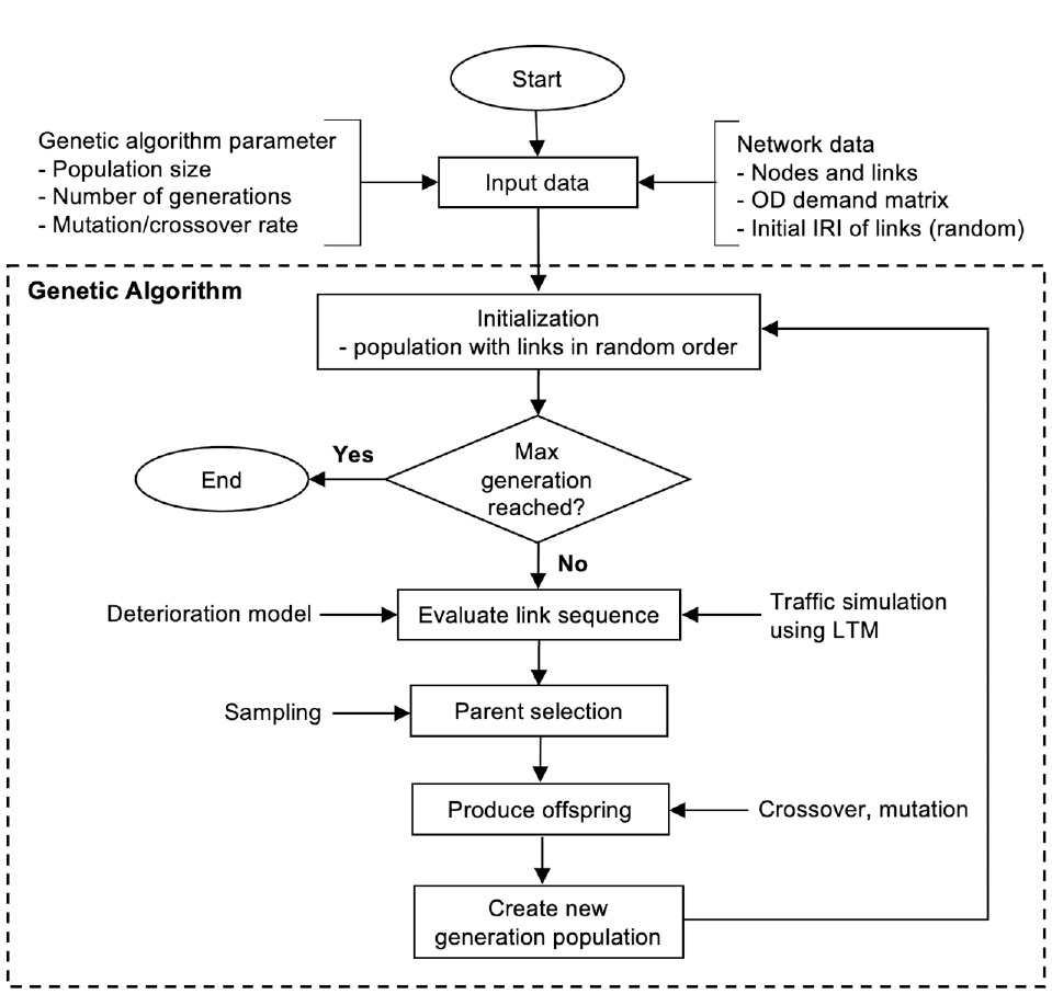
Flow chart of the methodology.
Genetic Algorithm (GA)
GA is a population-based meta-heuristic method that uses an iterative process to find the global optimum solution to an optimization problem. However, when the problem is highly complex, GA tends to converge at near-optimal solutions, which is the case in this study. GA is a versatile optimization algorithm that can handle discrete non-binary variables effectively and explore the solution space efficiently. It provides a good balance between exploration and exploitation, which is crucial for finding near-optimal solutions in complex problem domains in a limited time frame. GA offers versatility, global search capability, parallelism, robustness, ability to handle stochasticity, and effective constraint handling. These advantages make GA a powerful optimization method, particularly suitable for complex problems with discrete non-binary variables. At each iteration of GA, a population of possible solutions is maintained, where each solution is known as a chromosome. Chromosomes evolve according to principles from natural selection—that is, the fittest survive—and evolutionary genetics that change the chromosomes include crossovers and mutations.
Here, each chromosome represents a solution, that is, a maintenance schedule. It is assumed that
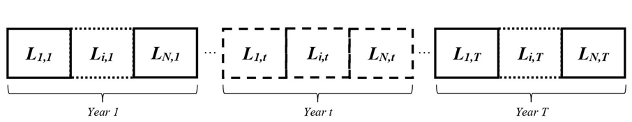
Chromosome with sequence of links representing a solution.
The fitness (or value) of a given chromosome is calculated using an evaluation model. The evaluation model computes the value of the objective function in dollars given a sequence of maintenance activities on the planning horizon. A multi-objective function used to evaluate the sequence has three components—the agency cost, the travel time cost, and fuel consumption cost. The objective function is formulated as follows:
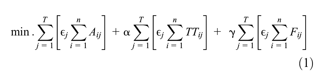
where
The agency cost depends on the maintenance activity chosen for a link, which is pre-determined based on the condition of that link. The second term represents the travel time costs from a total number of
The goal of the GA is to find the chromosome with the lowest objective value. To do so, an initial population of chromosomes is generated and evaluated using the evaluation model. The chromosomes with the lowest cost are selected to move on to the next generation. Next, crossover and mutation are applied to evolve the population. Crossover is a pairwise operation between two randomly selected chromosomes from the ones chosen to move to the next generation. A series of genes are interchanged between the two chromosomes and arranged by a crossover point based on the specified crossover rate. To avoid infeasible solutions with repeated link numbers, two advanced crossover techniques—ordered crossovers and partially mapped crossover—are implemented. This crossover process results in two unique chromosomes that represent a feasible solution to the objective function. On the other hand, mutation randomly changes a gene, resulting in a new chromosome. This process is repeated over a certain number of generations.
Evaluation Model
The evaluation model computes the value of the objective function (see Equation 1) in dollars, given a sequence of maintenance activities on the planning horizon. The evaluation model consists of the agency cost, travel time cost, and fuel consumption cost. Each of the costs are described below.
Agency Cost
The agency cost is determined according to the maintenance activity chosen. Three maintenance activities are considered: 1) preventive maintenance, 2) minor rehabilitation, and 3) major rehabilitation. It is assumed that preventive maintenance can be applied to a pavement in good condition, minor rehabilitation can be applied to a pavement in fair condition, and major rehabilitation can be applied to a pavement in poor condition.
Travel Time Cost
The travel time cost is determined using LTM, which is a numerical solution to the kinematic wave problem that requires evaluating flows of vehicles at nodes of a network. To do so, LTM assumes a first-in-first-out (FIFO) traffic principle and propagates cars from one link to the other. The formulation of the LTM enables it to capture the impacts of realistic traffic phenomena, such as queue propagation, dissipation, and spillovers, that is consistent with traffic flow theory.
The inputs to the LTM are: 1) an origin–destination (OD) demand matrix, 2) the underlying network configuration (i.e., the links and the nodes of the network), 3) triangular fundamental diagram parameters for each link, and 4) the capacity of each link. There are three main functions used in the LTM, namely the sending flow, receiving flow, and transition flow functions, which are calculated at each time step at the nodes of the network.
where
kjam = the jam density,
a = set of incoming links at node joining incoming link i and outgoing link j, and
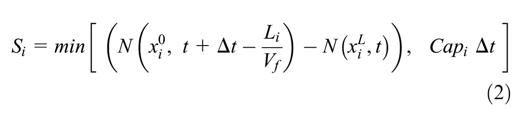
The sending flow is calculated at the downstream end of each link. It represents the maximum number of cars that are available to exit a link at the downstream end. The sending flow is constrained by capacity and traffic conditions at the link’s upstream end, as shown in Equation 2. The variable
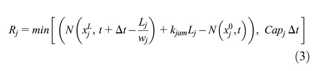
The receiving flow is calculated at the upstream end of each link. It represents the maximum number of cars that could enter a link, given a positive number of cars are ready to travel through the link. The receiving flow of a link is bounded by the capacity and traffic condition at the link’s downstream end, as shown in Equation 3. It is assumed that a congestion wave travels in the direction opposite to the movement of cars with a speed
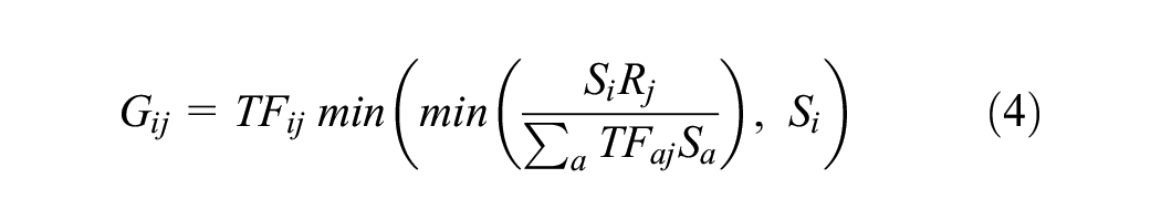
Unlike
The calculated transition flows are used to update the cumulative counts of cars at the upstream end of link j and downstream end of link i at every time step as
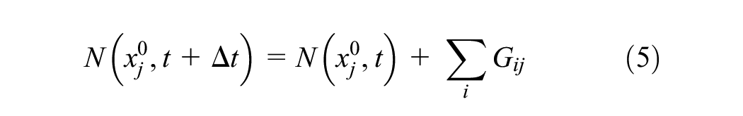
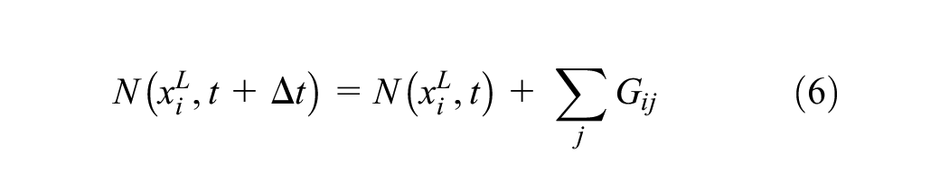
These cumulative counts are the main output from the LTM and are subsequently used to calculate the travel time on each link in the network. The link travel time is determined by considering the time difference between observing a given cumulative count of cars at the upstream of the link and the same cumulative count of cars at the downstream of the link. This is done by determining the time

Further, a route choice algorithm is employed in the LTM that allows commuters to change their route along the path with the shortest travel time between each OD pair, at regular intervals. This is assumed to mimic how cars would achieve user equilibrium in a network.
To evaluate the travel time cost for a given chromosome, it is assumed that maintenance is performed at the beginning of the year. To evaluate the total travel time per year, the LTM is run twice. One run is assumed to be representative of traffic when there is no maintenance, and the other run is assumed to be representative of traffic when there is maintenance. Therefore, while for the first run the full capacity of the links are utilized, for the second run the capacity of links on which maintenance is performed is reduced. The total travel time over a year is evaluated using Equation 8:
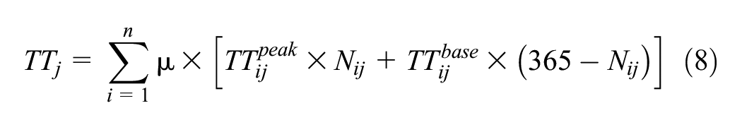
where
Fuel Consumption Cost
The fuel consumption model takes as an input the IRI of the link, the average speed on the link, and the volume or the number of vehicles using the link. The fuel consumption cost is calculated as follows. First, the energy consumption of vehicles on an individual link of the network is determined using Equation 9, which is borrowed from Santos et al. ( 54 ). The energy consumption is then converted to equivalent gallons of gasoline by dividing the energy consumption by the calorific value of gasoline. Next, we estimate the total fuel consumption cost by using the unit cost of gasoline (in $/gallon). The fuel consumption cost for each link is then multiplied by the volume of cars on each link and summed over all links in the network to get the total fuel consumption cost for the network.
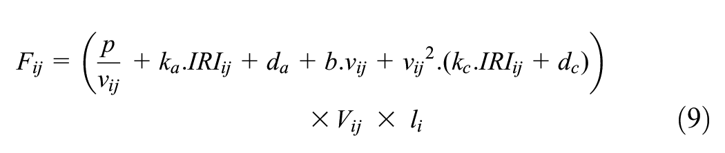
where
The average speed and the volume of cars on a link for a given year is determined using the LTM using the two runs of the LTM discussed in the previous subsection. The IRI of the link is determined using a deterioration model, discussed next.
Deterioration Model
To evaluate the fuel consumption cost and choose the appropriate maintenance activity for each link, the IRI values of links need to be determined over time. Therefore, a deterioration model is implemented to calculate how IRI increases over the years. Here, a linear deterministic deterioration model, borrowed from Santos et al., is used ( 54 ). It is worth noting that the methodology can work with other deterioration models, too. To account for variables such as traffic volume, weather condition, and so forth, on pavement deterioration, a more sophisticated model can be used. The current model was used for urban roads originally, shown in Equation 10:

where
Each year it is assumed that an unmaintained link deteriorates according to Equation 10, whereas maintained links improve their IRI based on the type of maintenance activity performed.
Numerical Example
To demonstrate the effectiveness of our proposed methodology, several assumptions were made. These assumptions include the consideration of only passenger car vehicles, a vehicle occupancy of one, and an equal valuation of time for all users. Additionally, we assumed that the fuel cost is calculated uniformly for all cars. While these assumptions may not capture the full complexity of real-world scenarios, they allow for a more manageable and standardized analysis, facilitating the examination of key factors in pavement maintenance decision-making.
A modest
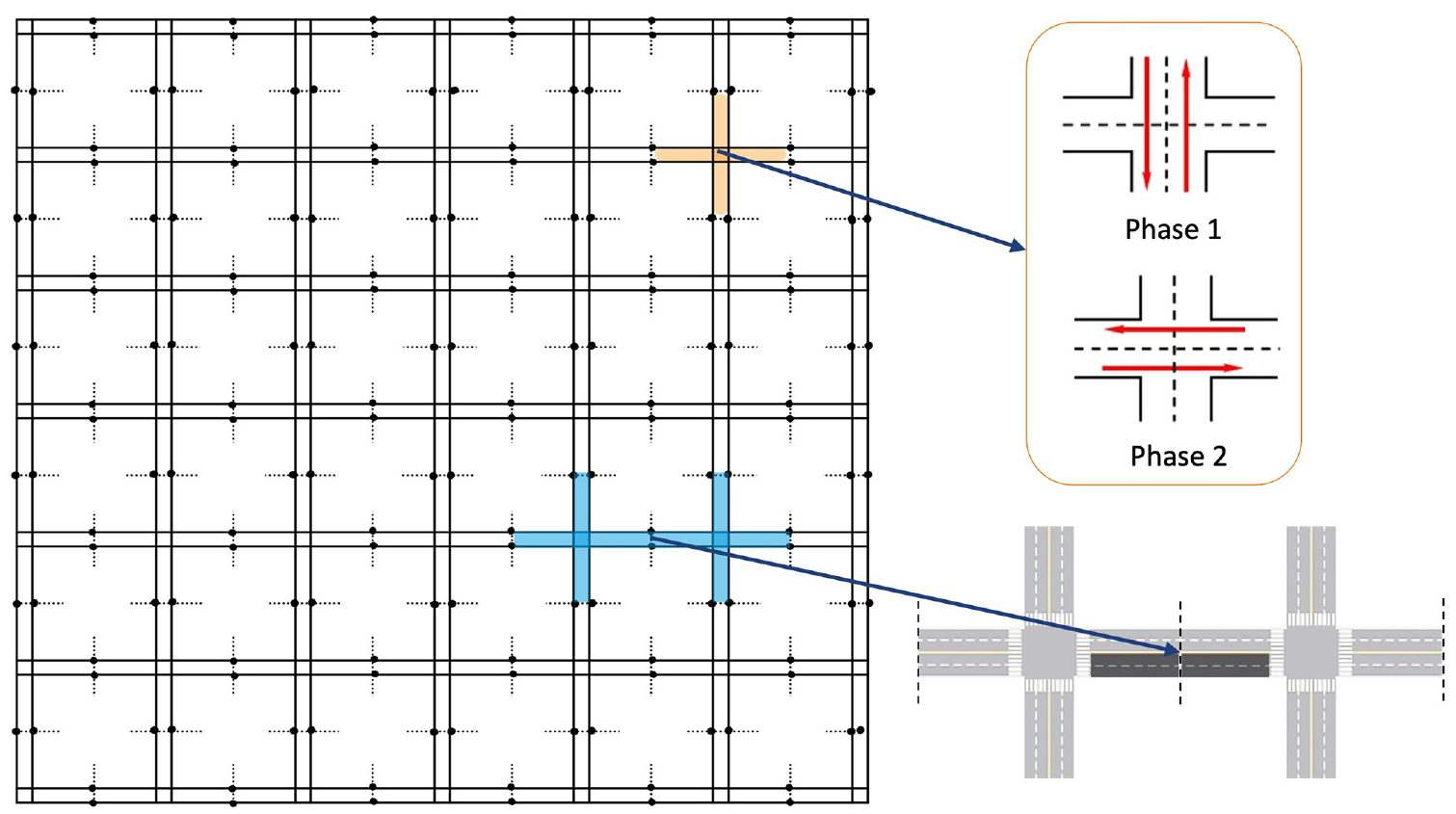
Illustration of the network, signal phase, and arterial link.
For initial pavement conditions at the first year, each of the 336 links in the network were randomly assigned IRI values that were uniformly distributed between 70 in./mi and 200 in./mi, ensuring the need for repair for some pavements while some remain in good condition. The IRI ranges of good, fair, and poor condition are determined according to the Federal Highway Administration (FHWA) technical brief HIF-16-032 “Measuring and Specifying Pavement Smoothness” ( 55 ). However, for evaluation of real networks, pavement evaluation results (say, IRI measurements) can be used instead.
Two 5-year planning scenarios with slower and faster pavement deterioration are considered in this numerical example. For both scenarios, 14 links are maintained each year, resulting in a total of 70 links that are maintained over the planning horizon. This deliberate decision represents a budget constraint, as it limits the scope of maintenance activities to a specific number of links within the available resources. By maintaining a fixed number of links, we aim to provide a simplified representation of the budgetary limitations faced by professionals and agencies in road pavement management. However, the methodology could be extended to explicitly consider budget constraints. The value of
The GA initializes with a randomly generated population size of 100 chromosomes with each chromosome containing a unique sequence of the selected links. The number of generations was set to 100 with a population size of 200 in every generation. The crossover and mutation rates were set to 70% and 1.43%, respectively.
To evaluate each sequence/chromosome, the traffic is simulated using LTM with a time-varying demand spanning across a 60 min time interval. For example, in the first year, the network is first loaded with cars by uniformly increasing the demand from zero to the full demand level for the first 15 min. Thereafter, the peak demand is kept constant at the rate of 20 cars/min per OD pair. The demand then gradually decreases to 5 cars/min in the final 15 min. The simulation runs until the network is empty. At the end of the simulation, the network travel time and peak hour volume is computed considering minutes 30 through 45 of the simulation. This is assumed to be the stable traffic condition that would be observed during the peak hours when maintenance activities were performed. In the subsequent years, the peak demand increases at the rate of 4% annually. Note that, since there is no randomness in the outputs of the LTM, for each year the model is only run once for evaluating the objective costs while links are under maintenance. A 60 min simulation is used to represent the largest impact the maintenance activities will have on traffic during the peak hour. Since the focus of this study is to present a methodology to address the maintenance scheduling problem while accounting for shock waves and queue spillbacks, the impact on peak hour traffic is assumed to be the most relevant. Such modeling has been shown to be superior to those treating traffic through static conditions that neglect the effects of bottlenecks and resulting queue spillbacks and overlook the traffic dynamics (
56
). Therefore, the peak-hour travel time is calculated and scaled to represent travel time during maintenance activities and the base travel time is used for the rest of the year to calculate the objective function. Moreover, it is assumed that the inflation does not influence the selection of maintenance actions, therefore,
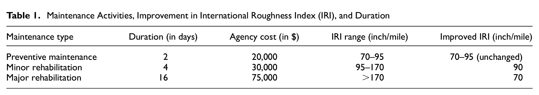
The duration of each maintenance activity, respective agency costs, IRI ranges to select maintenance activity type, and corresponding improvement in IRI are represented in Table 1, borrowed from Chao et al. ( 57 ). It was assumed that preventive maintenance does not help in improving the IRI of a pavement but prevents the pavement from further deterioration in the current year. Minor rehabilitation is applied to selected pavements with IRI between 95 in./mi and 170 in./mi. Minor rehabilitation is expected to improve the condition of a pavement by decreasing the IRI to 90 in./mi. Similarly, major rehabilitation is expected to decrease IRI of a pavement to 70 in./mi and is applied to pavements having IRI greater than 170 in./mi. Major rehabilitation can be thought as pavement reconstruction. The assumed values for the changes in IRI reflect the expected improvements that would be observed in the real world.
Maintenance Activities, Improvement in International Roughness Index (IRI), and Duration
Results
Figure 4 shows the change in the total travel time cost and fuel cost as the algorithm converges to an optimum solution for both cases considered. First, note that the travel time cost is much larger than the fuel cost—the first is in the order of millions while the latter is in the order of thousands. Therefore, the total cost is mainly driven by the travel time cost. However, different weights for each cost component could be considered if an agency would like to value fuel cost more than travel time cost. Further, the results show that, with each generation of GA, the travel time cost monotonically decreased but the fuel cost did not show a trend. In other words, sometimes the algorithm chooses a solution that decreases the travel time cost at the expense of the fuel cost. It can be said that, except some subtle differences, the general trends remain similar between the slower and faster deterioration cases. The increase in fuel consumption cost was also observed in the subsequent generations of the GA. This still leads to a lower total cost (see Figure 5) since the travel time cost component is much greater than the fuel cost.
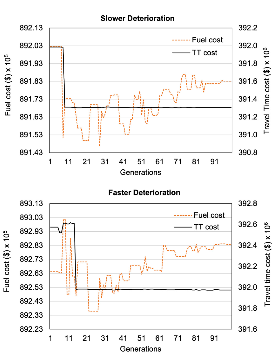
Travel time and fuel cost over the generations of the genetic algorithm (GA) in slower deterioration (top) and faster deterioration (bottom).
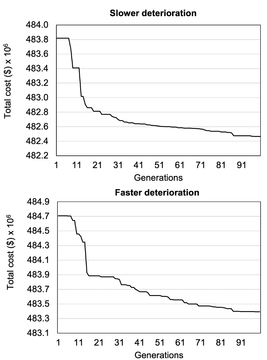
Convergence of total cost with slower deterioration (top) and faster deterioration (bottom).
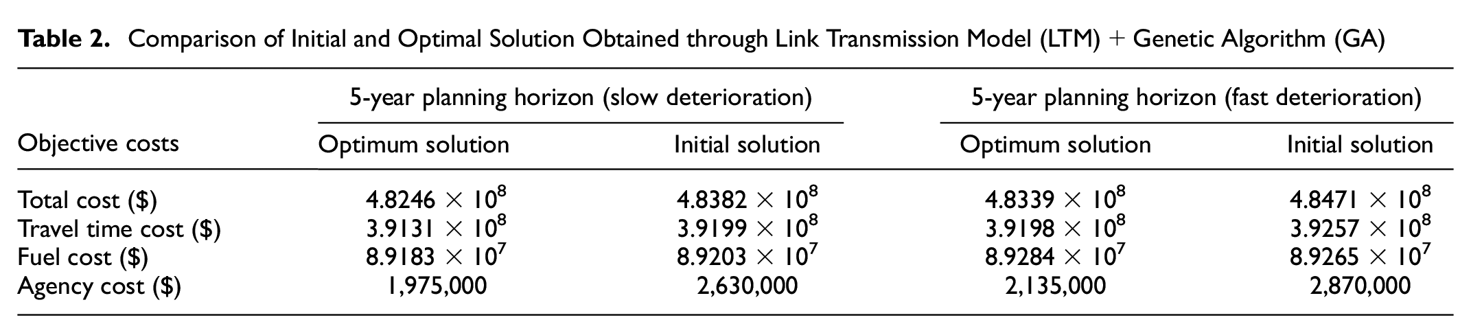
In this work it is assumed that the travel time on the network is independent of the pavement condition, that is, IRI. A comparison between initial and optimal solutions obtained through GA is represented in Table 2. The relative difference between the travel time cost can be related to about 680,000 hrs and 590,000 hrs in travel time savings in slower and faster deterioration cases, respectively. On the other hand, no savings were observed in the fuel cost in either case. Although the travel time and fuel savings were calculated as the difference between the solutions from the first and last generations of GA, it still provides a rough estimate on the levels of cost savings that can be attained using the proposed framework.
Comparison of Initial and Optimal Solution Obtained through Link Transmission Model (LTM) + Genetic Algorithm (GA)
To assess the overall condition of all the links in the network, average IRI is calculated and compared with the do-nothing scenario. Figure 6 compares the IRI for do-nothing and maintenance actions for the two deterioration scenarios. An improvement of 14.7 in./mi and 9.6 in./mi in average IRI was achieved for the entire network at the end of 5-year periods considering slower deterioration and faster deterioration, respectively.
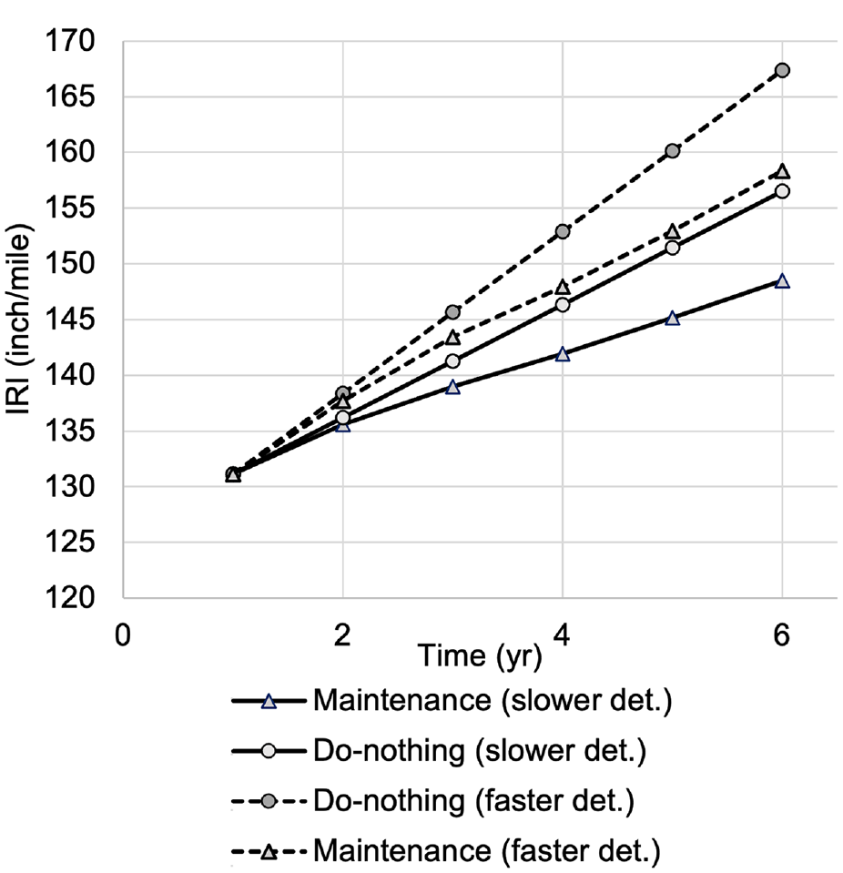
Average International Roughness Index (IRI) considering do-nothing and maintenance actions.
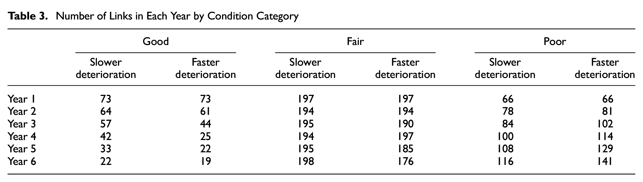
Table 3 illustrates the distribution of pavements in different conditions (good, fair, and poor) over a span of 5 years, considering two deterioration cases. The analysis reveals significant patterns in the network’s condition during this period. Specifically, the number of links categorized as “good” exhibits a consistent decline over the 5-year timeframe. Conversely, the number of links classified as “fair” remains relatively steady throughout the observation period. In contrast, the number of links falling into the “poor” category shows a notable increase over time. It is crucial to recognize that the chosen approach of maintaining a fixed number of links, specifically 70 out of a total of 336 in the network, might be insufficient to address the entire spectrum of deteriorating pavements adequately. The limitations imposed by the fixed number of links selected for maintenance become apparent as the proportion of pavements in good condition decreases and the number of poor-condition links increases. With a substantial number of pavements not included in the maintenance schedule, their deterioration progresses, contributing to an overall decline in the network’s condition. By implementing the derived maintenance schedule, even with a fixed number of links, the network benefits from the preservation of a certain proportion of pavements in fair condition. Although the overall condition of the network may still experience a decline, the rate of this decline is slower than it would be without any maintenance efforts—that is, the do-nothing scenario—as depicted in Figure 6.
Number of Links in Each Year by Condition Category
Further, the results from the proposed methodology were compared with a maintenance scheduling scenario without accounting for traffic dynamics and assuming cost of travelling on a link to be a convex non-decreasing function. The widely adopted Bureau of Public Roads (BPR) function was used in place of the LTM to calculate travel time on links, as shown in Equation 11. Table 4 compares the objective costs obtained using both the approaches. The objective costs from BPR-based model are relatively lower than LTM-based models. Given that both LTM- and BPR-based models converge to sub-optimal solutions, the difference in objective cost is mainly because of the inability of the BPR function to estimate travel time accurately, especially in situations such as congestion and queue spillbacks where travel time and fuel costs are significantly underestimated. Further, the BPR function, because of its convex nature, also overestimates the travel time during free flow condition in a link. Therefore, the LTM-based model is expected to represent more realistic fuel cost and travel time cost by accounting for congestion and queue spillbacks. Also, the LTM accurately estimates the travel time in free flow conditions. Table 4 shows the comparison of objective costs obtained from LTM- and BPR-based models considering slower and faster deteriorations. Comparing the two deterioration rates, we observe that the LTM-based model results in lower travel time cost in slower deterioration, while a higher travel time cost in the faster deterioration. Fuel costs calculated using the LTM-based model is greater than the BPR-based model in both the scenarios. The observed trends between the LTM- and BPR-based models are mainly because of the difference in link volumes calculated using BPR and LTM. The LTM results in relatively high volumes because of congestion and queue spillbacks as a result of which the fuel cost increases. The link volumes calculated using the LTM formulation depict a better representation of traffic flows in the network; therefore the objective costs calculated using the LTM-based model account for traffic dynamics, congestion, and queue spillbacks. Despite the opposite trends in travel time cost and agency cost, the total costs obtained through the LTM-based model are relatively higher than those obtained using the BPR-based model in both cases.
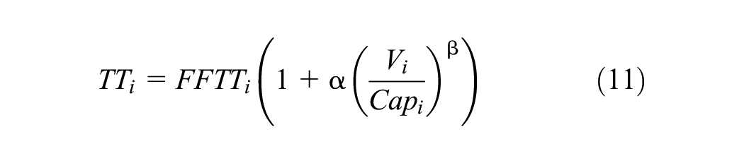
where
Optimal Costs Obtained through Link Transmission Model (LTM) + Genetic Algorithm (GA) and Bureau of Public Roads (BPR) + GA Considering Slower and Faster Deterioration
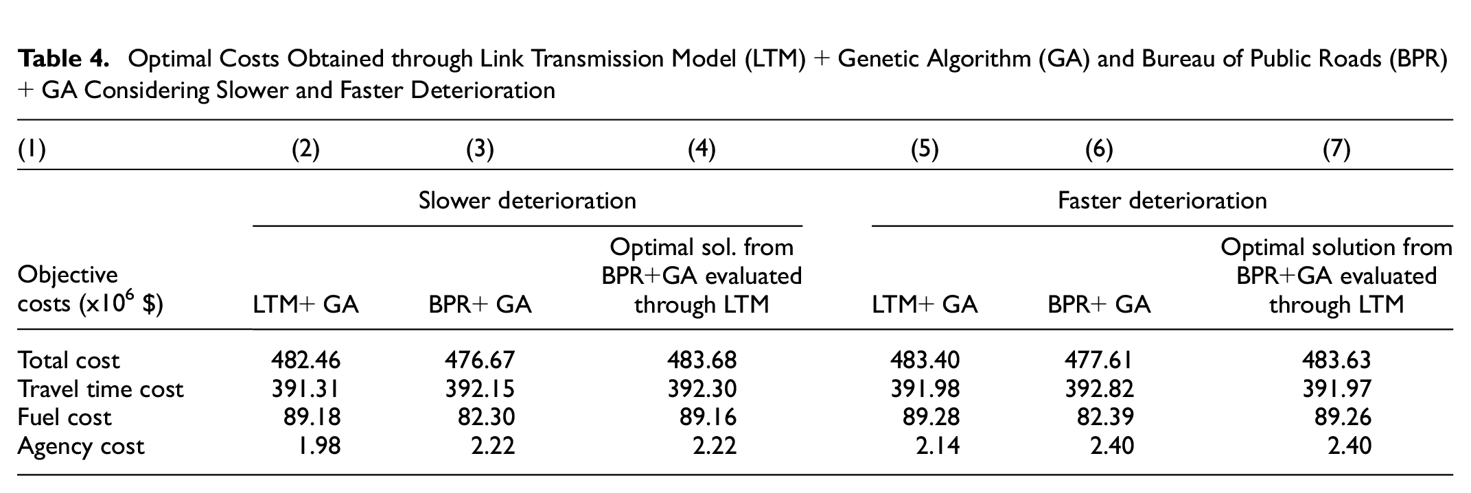
The solution obtained through the BPR-based model was evaluated using the LTM-based model to compare the two approaches. Since the BPR function does not account for queue spillbacks, it underestimates the total cost in both the scenarios. Queue spillbacks have been known to increase the total travel time in a link mainly because of cars waiting in the queue. It is evident that the LTM-based model results in higher travel time cost and fuel cost compared with the BPR-based model, considering a specific sequence of links to maintain (Table 4, columns 2 & 4 and 5 & 7). Furthermore, when comparing the solutions obtained from the LTM- and BPR-based models (Table 4, columns 2 & 3 and 5 & 6), it can be concluded that the LTM + GA model performs better at minimizing traffic disruptions, as we see from the lower travel time cost achieved by the LTM-based model compared with the BPR-based model. The ability of the LTM-based model to consider queue spillbacks and account for resulting delays contributes to its effectiveness in reducing overall traffic disruption during the selection and sequencing of maintenance activities.
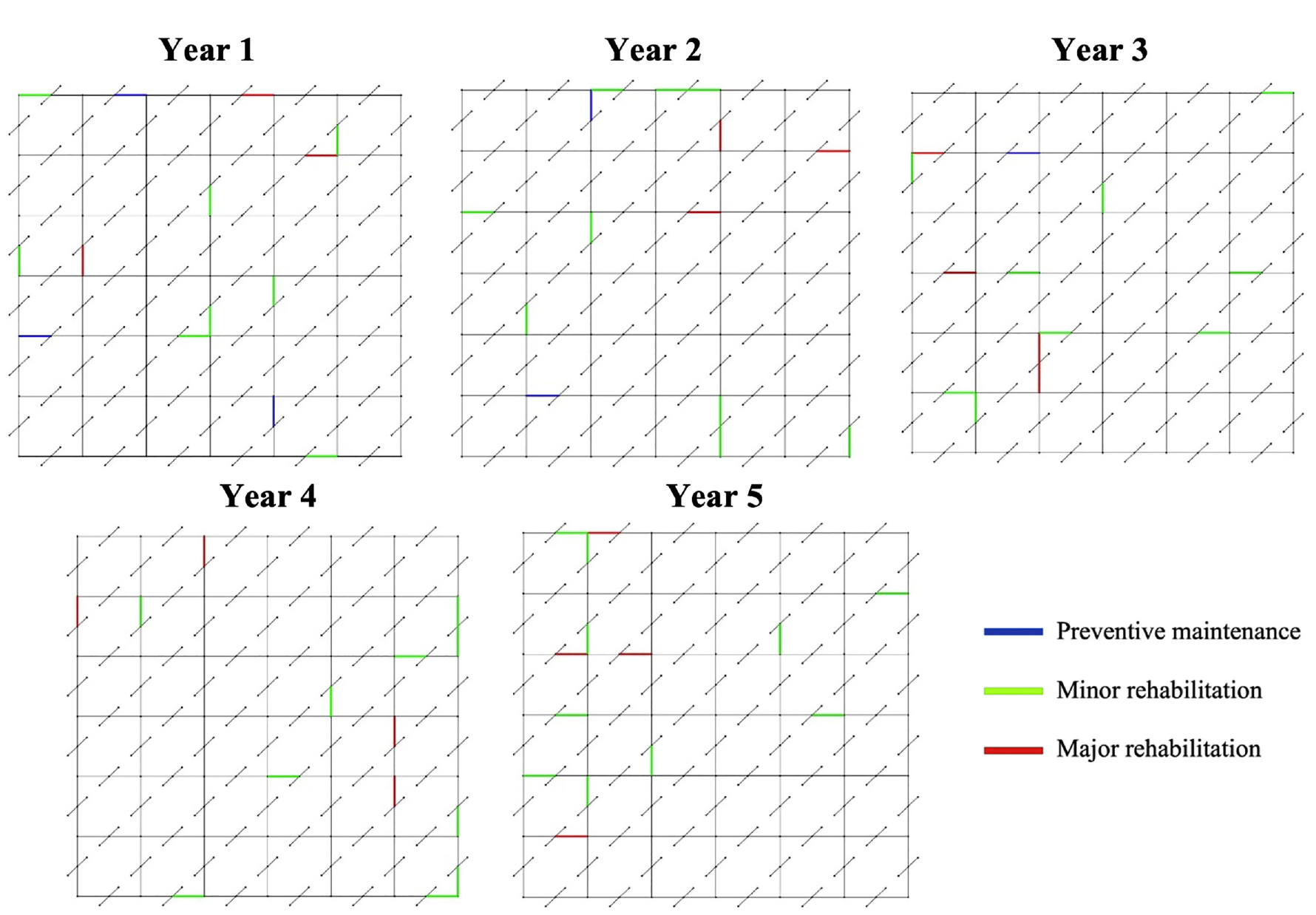
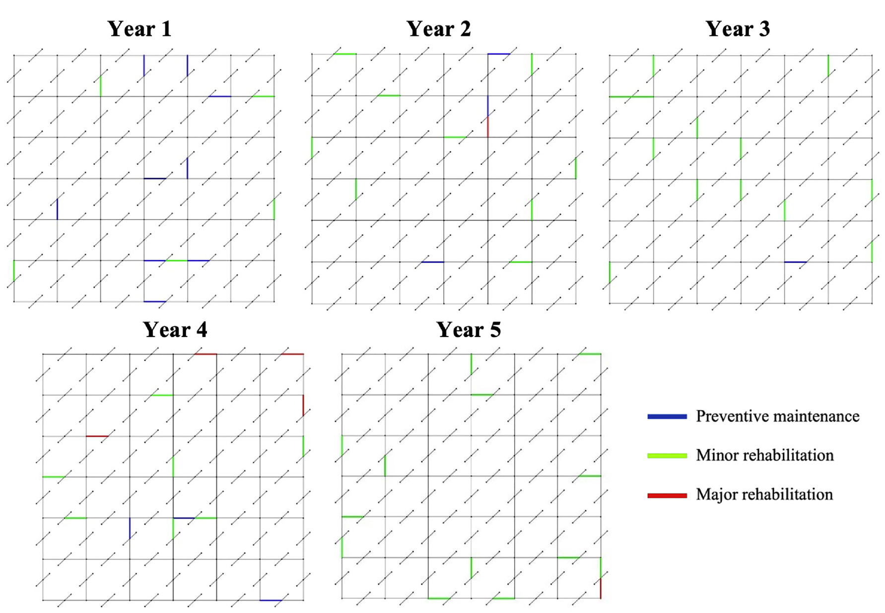
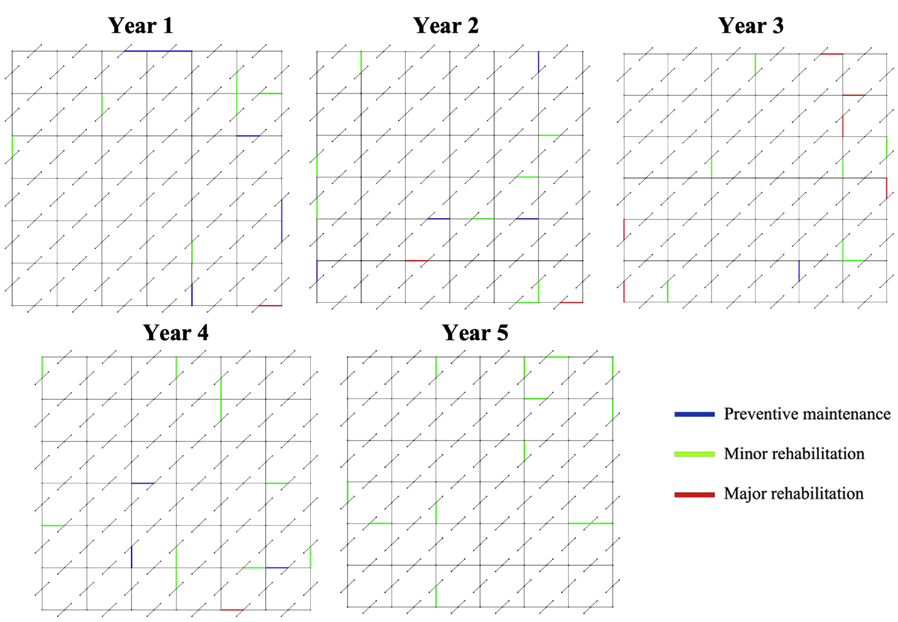
The links selected for maintenance each year considering slower deterioration as obtained through the LTM- and BPR-based models are shown in Figures 7 and 8, respectively. It is observed that the solutions (i.e., sequence of links to maintain) obtained from the two approaches are remarkably different. A similar observation was recorded in the scenario with faster deterioration, and the links selected for maintenance each year are represented in Figures 9 and 10.
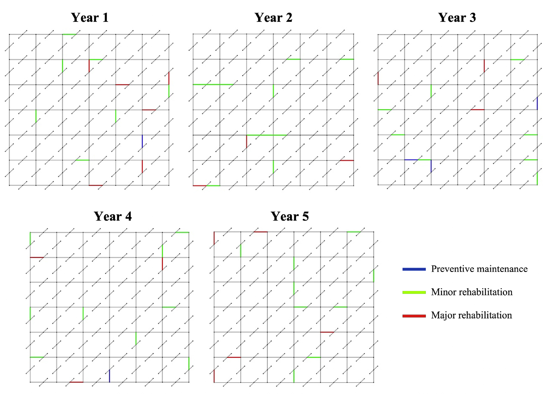
Maintenance scheduled derived using the link transmission (LTM)-based model considering slower deterioration.
Maintenance scheduled derived using the Bureau of Public Roads (BPR)-based model considering slower deterioration.
Maintenance scheduled derived using the link transmission (LTM)-based model considering faster deterioration.
Maintenance scheduled derived using the Bureau of Public Roads (BPR)-based model considering faster deterioration.
Limitations
A notable limitation of this study is the absence of a constraint on the network-wide pavement condition. As a result, the algorithm prioritizes maintenance actions that are less costly overall, aiming to improve the objective function while also performing costly maintenance actions when needed. This leads to a decrease in agency cost over the generations of GA. This limitation highlights the need for future research to consider incorporating constraints related to the pavement condition into the decision-making process. By incorporating such constraints, the algorithm can ensure that maintenance actions are selected in a manner that not only optimizes the objective function but also takes into account the condition of the entire pavement network. This would provide a more comprehensive and realistic approach to pavement maintenance planning. Future works should address this limitation to further enhance the methodology and its practical applicability.
Additionally, it is important to acknowledge that pavement deterioration is a complex and stochastic process. Currently, the proposed methodology assumes a deterministic deterioration model, which does not fully capture the inherent variability and uncertainty in pavement deterioration. To address this, future works will consider incorporating a stochastic deterioration model into the maintenance scheduling process. By accounting for the probabilistic nature of pavement deterioration, the methodology can provide a more accurate and reliable assessment of the optimal maintenance sequence.
Another significant limitation of the proposed methodology is the exclusion of certain costs, such as environmental or emission costs and safety costs, from the objective function. Incorporating such costs would enable the evaluation of the environmental impacts associated with different MR&R activities. This could involve considering factors such as greenhouse gas emissions and air pollution, allowing decision-makers to prioritize environmentally friendly maintenance strategies. Safety costs are equally critical and encompass various aspects, including crash rates, injury severity, and crash costs. Incorporating safety costs into the objective function would provide a comprehensive assessment of the impact of MR&R activities on overall road safety.
Conclusions
This study introduces a novel methodology for addressing the challenge of scheduling maintenance activities at a network-wide level. While previous research has attempted to tackle this issue, it has often neglected to account for the bottlenecks arising from traffic disruptions caused by reduced link capacity or link closures during maintenance operations. Consequently, a notable gap exists within the existing literature. We address this gap by implementing a traffic-flow-theory-based model that is capable of considering the impacts of traffic scenarios such as shockwaves and queue spillovers. For this, we employ an LTM in conjunction with a GA to derive the optimized schedule of maintenance activities over a defined planning horizon. The GA’s distinctive capabilities in exploring and exploiting solution spaces render it a robust optimization technique, particularly suited for intricate problems involving discrete non-binary variables. The LTM simulates traffic on the network and is capable of capturing queue spillovers. Given the underlying computational burden inherent in traffic dynamics, the proposed methodology was tested on a simple grid network to demonstrate the approach. In this study, the travel time component carries more significant weight in the overall objective function; however, different weights for each cost component could be considered if an agency would like to value certain costs more. The benefits of selecting and maintaining links in the optimal order derived can be represented in travel time and fuel saving. As demonstrated in the numerical example, the proposed framework accounts for traffic congestion and queue spillbacks, and thus better estimates the travel costs. The difference in the objective cost obtained using LTM- and BPR-based models can be related to over 7,000 h of travel time and over 1.5 million gallons of fuel, which was underestimated by the BPR function during the process of MR&R planning for 5 years in the future. Also, the solutions obtained through LTM- and BPR-based models are significantly different. In other words, a unique set of links was selected for maintenance using the two approaches. The LTM-based model accurately estimates the objective costs, while the BPR-based model fails to do so. Therefore, the proposed framework can be used to account for traffic phenomena such as congestion, shockwaves, and queue spillovers in long-term pavement MR&R. The incorporation of different costs into the objective function, such as environmental and safety costs, to encompass more realistic networks will be considered in future studies.
Footnotes
Author Contributions
The authors confirm contribution to the paper as follows: study conception and design: A. Prajapati, A. Sengupta, S. Guler; data collection: A. Prajapati, A. Sengupta, S. Guler; analysis and interpretation of results: A. Prajapati, A. Sengupta, S. Guler; draft manuscript preparation: A. Prajapati, A. Sengupta, S. Guler. All authors reviewed the results and approved the final version of the manuscript.
Declaration of Conflicting Interests
The author(s) declared no potential conflicts of interest with respect to the research, authorship, and/or publication of this article.
Funding
The author(s) received no financial support for the research, authorship, and/or publication of this article.