
Abstract
Highway pavements deteriorate over time as successive wheel loads cause rutting, cracking, texture loss, and so forth. Design standards and pavement performance models account for some of the known contributory factors, such as levels of traffic and vehicle composition. However, such models are limited in their predictive power, and highway authorities must conduct regular pavement condition surveys rather than relying on the standard deterioration models alone. The ways in which multiple factors affect pavement deterioration, including rutting, are complex and are believed to include feedback loops where rutting then influences driving position, exacerbating the rutting levels. Standard regression models are not well suited to representing such complex causal mechanisms. This paper compares two alternative modeling approaches, structural equation models and auto-machine learning, and evaluates the predictive ability and practicalities of each. The findings indicate that auto-machine learning (AutoML) may be superior in its predictive ability. However, the “black box” nature of AutoML results makes them potentially less useful to practitioners. A process of using machine learning to help inform a structural equation model is proposed.
Keywords
Highways provide the means of transportation for most trips globally. Construction of such highway pavements is expensive, as is the ongoing maintenance that they require over their lifespan. Key to ensuring the performance of a pavement is predicting the increase of vehicle and axle load, extreme loads, environmental factors, construction errors, maintenance, and controls that the pavement will need to endure over its lifespan. There are several contributors to major pavement deterioration and consequently the lifespan of pavements. The key determinant has been found to be the amount of and type of traffic exerting a load on the pavement surface. Globally, studies and design codes have highlighted that load repetitions and distribution across the pavement surface by heavy vehicles results in considerable deterioration ( 1 , 2 ).
Rutting is a common deterioration mode of flexible pavement structures resulting from repeated load applications along the wheel paths ( 2 – 10 ). Previous research has suggested that there may be feedback loops in the causal mechanisms through which rutting and driver position (lateral wander) interrelate. The hypothesis is that, as rutting occurs, the wheels of vehicles are channeled into the ruts, which in turn exacerbates the rutting. There may also be complex feedback loops between geometric characteristics of the road, the vehicle positions, and rutting ( 11 ). However, in the United Kingdom (UK), design ( 12 ) and guidance ( 13 ) give little advice to engineers as to the relationships between highway geometries and the cross-sectional distribution of axle loads from vehicle positioning (lateral wander). Equally, there is little empirical evidence globally of the causal mechanisms by which geometry, vehicle position, and rutting interrelate ( 14 , 15 ). As such, the objective of this paper is to provide a means by which these complex interactions could be considered through piecewise structural equation modeling and through a form of artificial intelligence, using empirical data collected in Portsmouth, UK. The two approaches are compared for their predictive ability, their practicality, and the extent to which they can help pavement engineers design and maintain pavements better in the future. While the findings here provide interesting insights into the effects of different parameters on rutting, the scope of this paper is to compare and contrast the two alternative modeling approaches, to suggest a way in which rutting could be considered going forward, either by researchers or practitioners.
Standard Modeling Approaches
To understand relationships between multiple variables and to develop explanatory and predictive models, regression analysis is widely used ( 16 ). More specifically, regression analysis helps understanding of how the typical value of the dependent variable changes when any of the independent variables are varied. In all cases, the estimation target is the function of the independent variables called the regression function. In regression analysis, it is also useful to characterize the variation of the dependent variable around the regression function, which can be described by the probability distribution ( 17 ). Multivariate linear regression is used to develop a single equation from the set of independent variables ( 18 ). The relationship between the dependent variable and the independent variable is also assumed to be linear ( 19 ). In summary, the assumptions underpinning the multivariate linear regression analyses were: independence, linearity, normality, and homoskedasticity. In other words, the residual of a good model needs to be normally and randomly distributed ( 19 ).
In all statistical analysis the goal is generally to understand the relationships between the variables. Although multivariate linear regression analysis provides an overarching way to quantify the relationships and to determine the links between the independent and dependent variables or to specify the conditions under which the association takes place, there are some limitations. The assumptions of a normally distributed response variable and linear association between the predictors and the response can be overcome by using alternative forms of regression with different link functions. However, one of the biggest limitations of all standard multivariate analyses is that they can only demonstrate unidirectional relationships and they can only handle observed variables. In the context of rutting, research has demonstrated links between geometry, vehicle position, and rut depth. However, the vehicle positions have also been shown to relate to geometries ( 9 ), and in two cases to the rut depths ( 3 , 11 ) suggesting multidirectional relationships.
Review of the Modeling Approaches
Structural Equation Model: Path Analysis
Structural equation models (SEM) were developed to help address the limitation of standard regression models, by enabling more complex causal paths to be investigated. SEM is a multivariate technique that combines regression, factor analysis, and analysis of variance to simultaneously estimate interconnected dependent relationships ( 20 ).
Path analysis is a family of SEM, historically based on the work of Sewall Wright from the 1920s. He attempted to quantify the direct influence of one variable on another using path diagrams and correlations. As a result, the path analysis method depends on the degree of correlations in a system ( 21 ).
Wright obtained the fundamental formulation of path coefficients by describing the typical path diagram shown in Figure 1. Variables are linked to one another by one-way arrows resulting from dependent relationships. The double arrows reflect residual correlations between variables, and
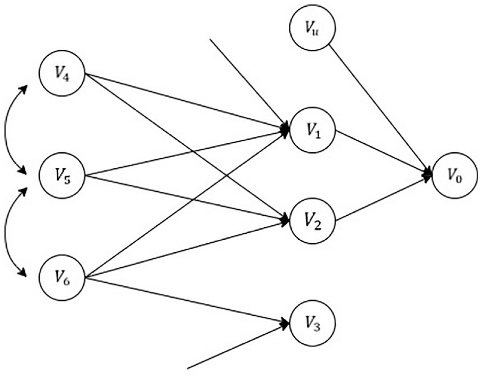
Path analysis diagram ( 22 ).
Each variable, when considered from a unidirectional point of view, results from the following.
where

where

where
Equations 2 and 3 can be arranged, respectively. Then, they can be combined with Equation 1 as follows:
In light of this, the most up-to-date form of the equations will look like this in the event that the superfluous parameters in the previous equation are removed:

Each path coefficient (
One difficulty in using SEMs to explore complex causal mechanisms is the high number of possible causal paths and explanatory variables that may exist. This may require a significant number of alternative specifications to be created and tested before a suitable model is found.
SEM has not been employed in the literature to examine the relationships between explanatory factors and rutting.
Multilayer Perceptron
Contrary to standard regression or SEM models, machine learning tools are increasingly used to predict outcomes, which might result from very complex underpinning causes. A feedforward artificial neural network (ANN) model, also known as a deep neural network (DNN) or multilayer perceptron (MLP), is the most common type of DNN (
23
,
24
). To understand why the MLP is necessary, it is important to comprehend the basic concept of neural networks. Figure 2 illustrates the working principle of a perceptron. The impulse (data) comes from the left side to the right side. All impulses sourcing from input variables (
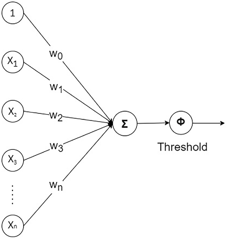
Illustration of perceptron.
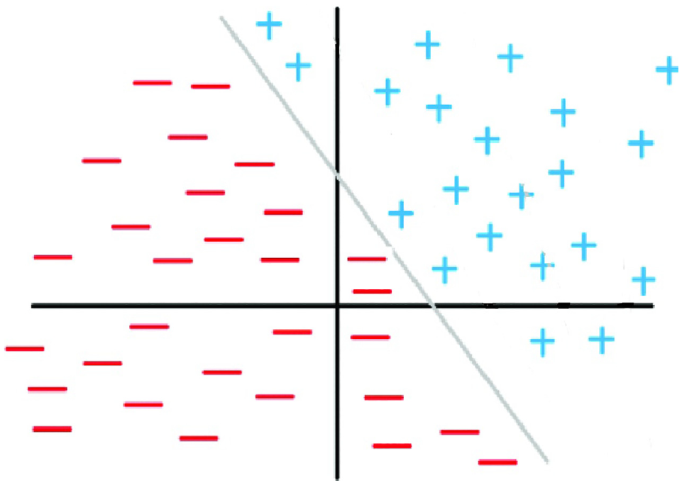
Linearly classified sample ( 25 ).
In Figure 3 the data appear to be clearly separated into two categories (plus signs and minus signs) and these categories are separated by a simple straight line. Where the separation of data is more complex (nonlinear or multidimensional) then an ANN is required.
The MLP was designed as a solution to the problems caused by the perceptron’s limited capabilities. In essence, it is a model for an ANN that consists of three or more layers. As a result, it can process information that cannot be partitioned linearly by a hyperplane ( 26 ). MLP utilizes a neuronal architecture known as feedforward, in which signals travel through the network in just one way, from input to output ( 27 ).
Training and Calculation of Predicted Values
When it comes to neural networks, one of the challenges that must be faced is determining the appropriate number of hidden layers and neurons. However, there is abundant evidence in the published research that demonstrates conclusively that there is no deterministic approach to determining the structure of neural networks. The specific number of hidden layers and neurons required to solve a problem will vary significantly from case to case. The designer is forced to settle on arbitrary decisions ( 28 ). Nevertheless, the AutoML algorithm can choose the most effective architectures ( 29 ).
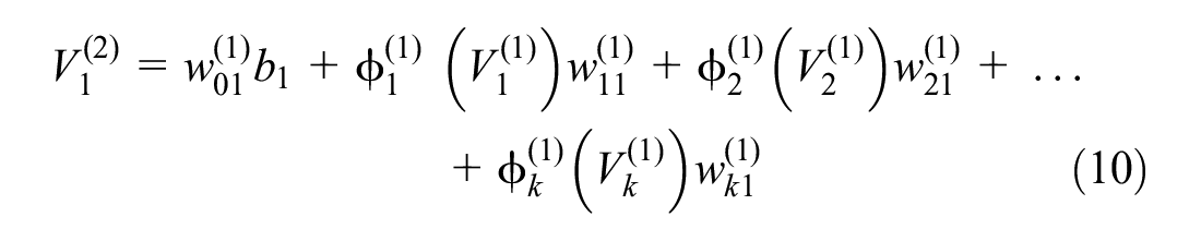
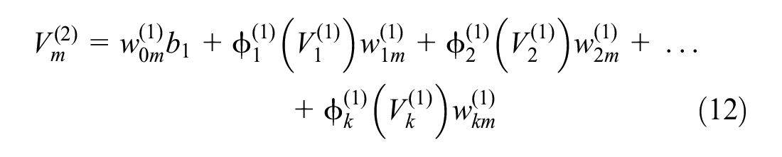
Figure 4 illustrates a typical neural network including n number of input variables, two hidden layers with k and m number of perceptions, and one variable in the output layer. Calculation of the predicted output variable (
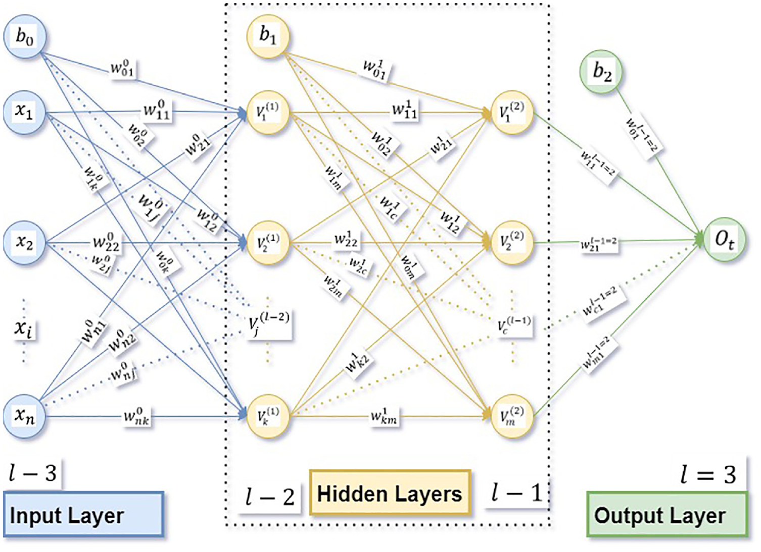
Illustration of neural network with two hidden layers.
Equations for weighted sum (


The above equations can be formulated as Equation 9.

where
Equations for weighted sum (
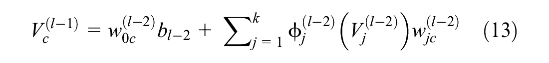
where
The last stage is to obtain the predicted value (
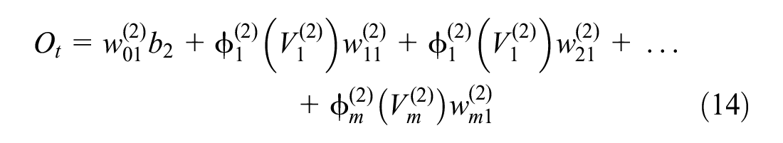
This can be written as follows:
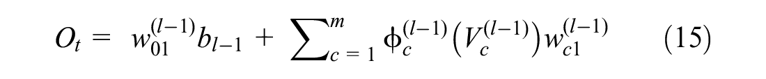
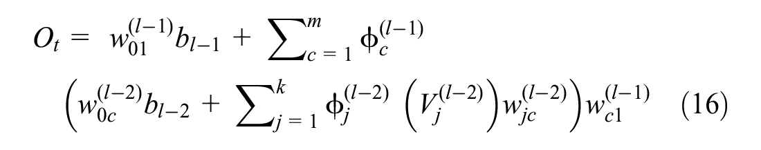

where
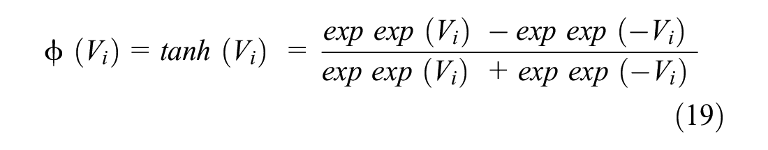
The nonlinear activation functions of the MLP is precisely what makes the model powerful. Almost all nonlinear functions can be used for this. Recently, one of the most commonly used functions is sigmoid ( 27 ).
Sigmoid activation function is as follows:

One of the commonly used alternatives is hyperbolic tangent:
As explained above, the output layer (

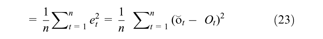
Error Computation
The sum-of-squares error of iteration can be computed as Equation 21:

where
Minimization of the error term
Model Performance
Model performance, predicted by an observed chart with an R-squared value, is a common way to determine the performance of the prediction ( 32 ). It can be calculated as follows:

where
Interpretation of Results
The issue of a “black box” arises when interpreting the findings of ANN models. The unfathomable hidden layer(s) of neural networks are regarded as “black boxes” in common parlance. It is impossible to provide a scientific explanation for what occurs in the hidden layer(s). However, to evaluate the model, a sensitivity analysis may be taken into consideration. A sensitivity analysis is a way of analyzing the behavior of a model and determining the degree to which each input (independent) variable is relatively essential. This can be accomplished by analyzing the model’s output, and it seems to provide insights into the usefulness of each input variable ( 33 ).
We have explained how sensitivity analysis could be implemented, as seen in Figure 5. The first step in this process, step (a), is to have a model including the whole input variable and the mean squared error (MSE) value of this model ( 34 ).
Mean Squared Error(MSE)
where
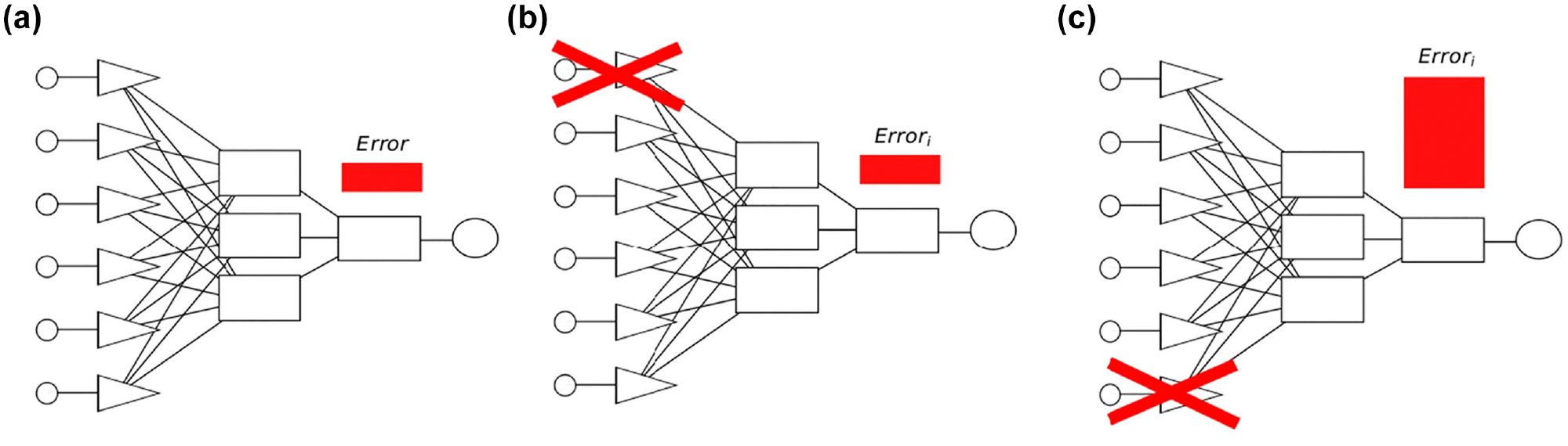
Process of sensitivity analysis ( 34 ): (a) The first phase of sensitivity analysis; (b) The second phase of sensitivity analysis; (c) The third phase of sensitivity analysis.
In the further steps (b, c…), input variables are removed from the model, and

where
H2O AutoML
H2O AutoML was introduced by Ledell and Poirier ( 24 ) as an open-source, scalable, and fully automated supervised learning algorithm implemented in the H2O distributed machine learning framework.
Many steps have been taken to develop user-friendly machine learning software. Even if these tools have made it easier for non-expert users to train machine learning models, they require a fair amount of expertise to achieve robust results ( 24 ). AutoML tools provide a simple interface for training multiple models, with different algorithms such as gradient boosting machine, random forest, DNN, and generalized linear modeling and can be a valuable tool for both novice and advanced practitioners of machine learning ( 24 ).
The algorithm adopted in this paper is DNNs. AutoML within R Studio was selected as it does not need human assistance to produce robust results ( 29 ).
The illustration provided in Figure 6 outlines the data collection and analysis process. This process started with gathering relevant data, including primary and secondary. Two distinct analysis techniques were selected for this study: SEM and AutoML. These were utilized using AMOS SPSS 28 and R Studio 2022.12.0, respectively.
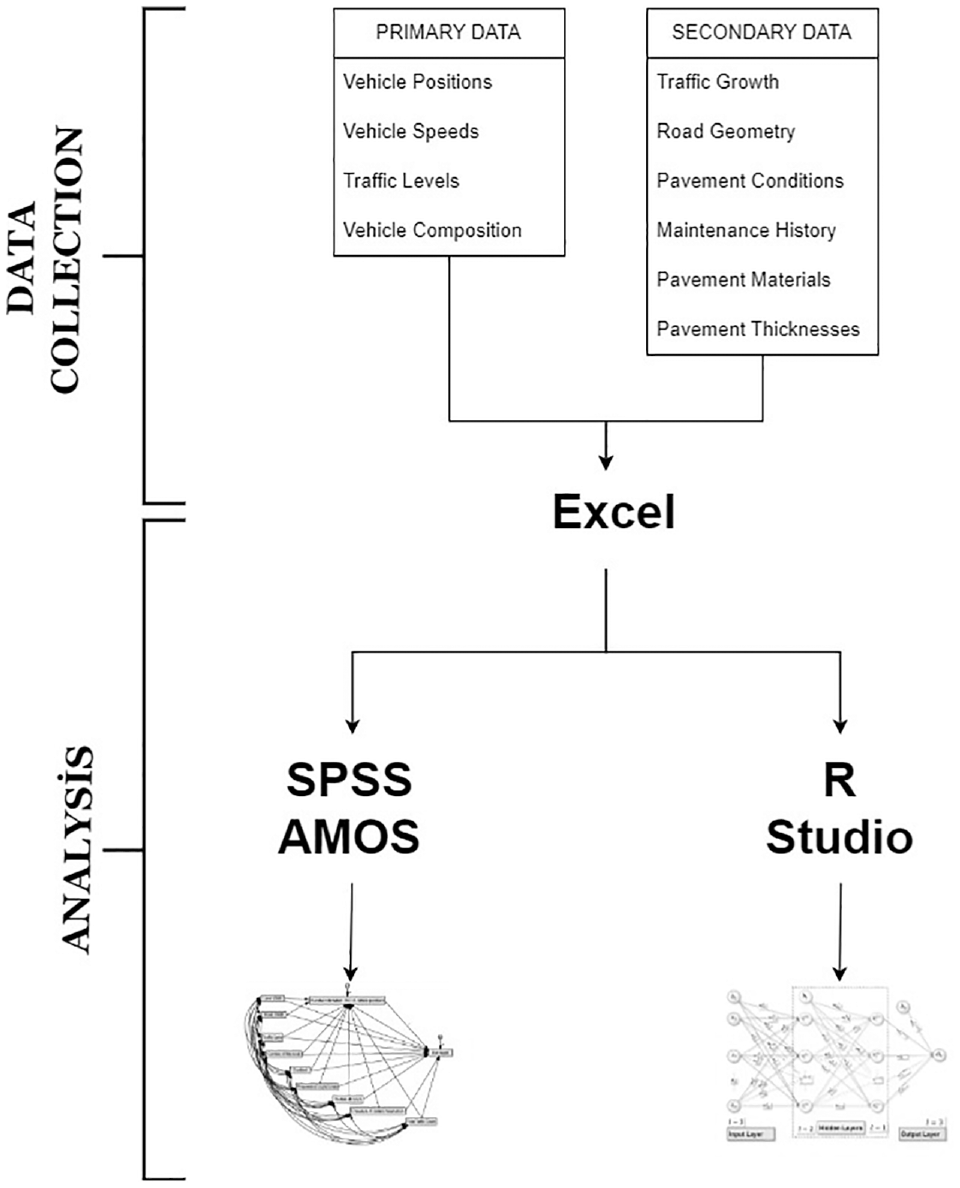
Flowchart of the method.
Case Study
Description of Data
Data were collected through observations from two primary roads, the A288 Clarence Parade and South Parade, stretching approximately 1,530 m (Figure 7). They were selected because the traffic flow/composition is similar along their lengths and there is no significant change in longitudinal road gradient. There was also minimal variation in climatic conditions along the length, while the geometry (width of lane and road, curvature and camber) and presence of road features varies considerably.
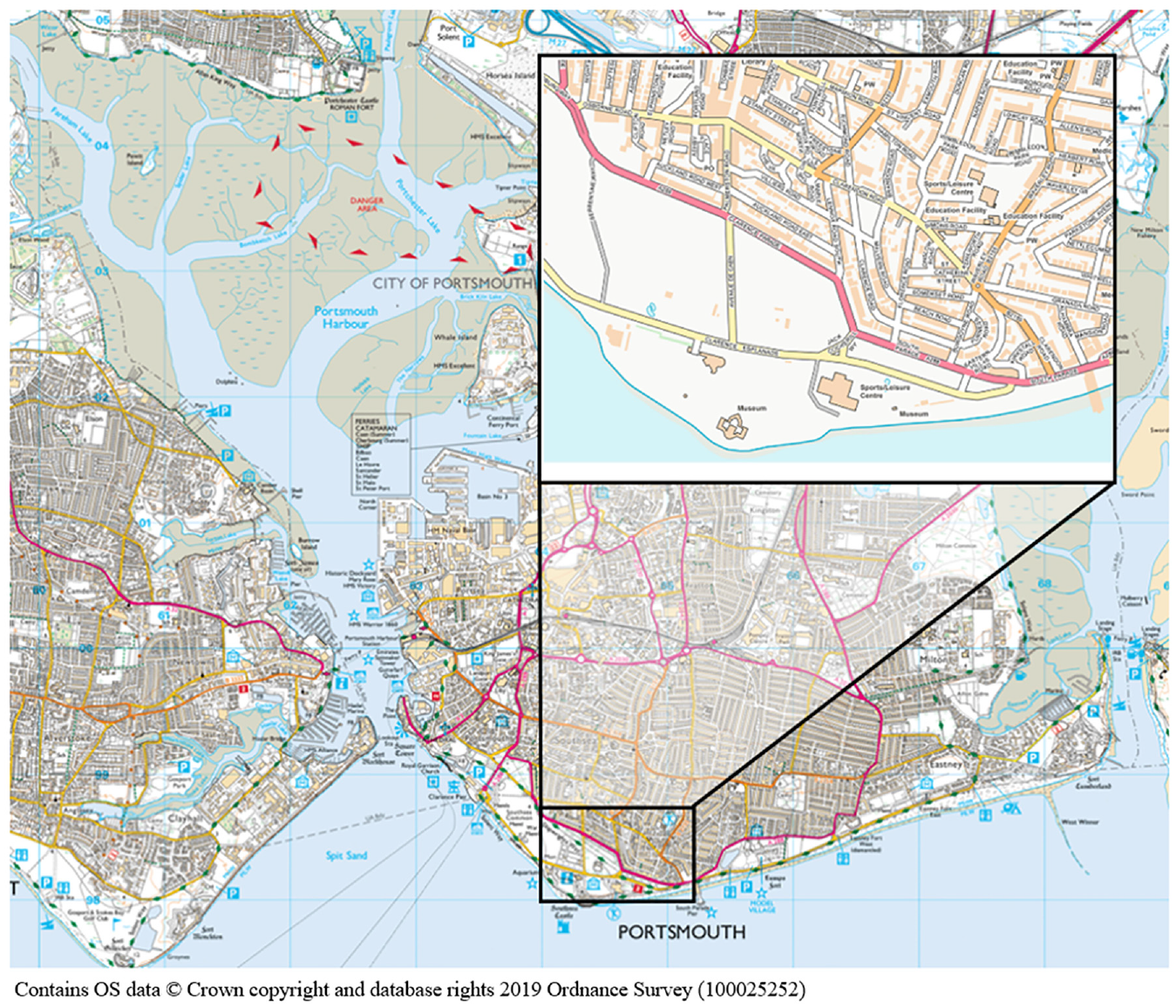
Location of study area in Portsmouth, UK: Clarence Parade and South Parade ( 35 ).
The research involved both primary and secondary data. The primary data were collected by measuring the lateral placement of vehicles under investigation. The details of this approach are described by Sinanmis and Woods ( 36 ). The overall road and lane widths were measured using a laser measuring device.
Secondary data were obtained from Portsmouth City Council and its highways contractor, Colas Ltd, through their regular surveys of road condition. This included SCANNER (Surface Condition Assessment for the National Network of Roads) survey data which is intended to provide a consistent method of measuring the surface condition of road carriageways, using automated road condition survey machines, throughout the UK ( 37 ). The SCANNER data were collected for different traffic lanes and directions for different years. The data for road conditions obtained from Colas include rut depths in millimeters for both wheel paths averaged over 10 m lengths. Camber (percentage cross fall) and horizontal curvature (radius of curve) were also collected from Colas as potential explanatory factors. All the data supplied by Colas were taken from three different survey years. As the case study is in the UK, vehicles drive on the left. The terminology used from here in this paper is that “curb-side” relates to the outer wheel path and “centerline-side” relates to the wheel paths closest to the road centerline.
When considering the lifespan or condition of a pavement, the average deterioration across the pavement is not of interest. What is important is that no section of the pavement falls below a certain level of performance. For this reason, the curb-side rut is usually the determining factor in the overall rut level on a road section rather than the (usually lower) right rut. As such, in this study the curb-side (left) rut was used in the analysis, rather than the centerline-side.
The SCANNER dataset also includes other potential explanatory factors for each of the 100 locations (circa 10 m intervals along the lengths of the case study roads) as follows:
Eastbound or westbound traffic lane.
Year of rut depth data (2014, 2017, 2018).
Camber (percent cross fall).
Horizontal curvature (radius of curve).
To match the primary data chainages with rutting data chainages, ArcGIS software was used to overlay rutting data onto the data collected in the field. The 100 observation points were matched to the corresponding rut depths through the use of ArcGIS software (version 10.6.1) and the coordinates of each point.
The annual average daily traffic (AADT) count was recorded, and it showed there was little difference in eastbound and westbound lane flows.
Construction of Models
Figure 8 depicts the construction of the regression model based on path analysis. It was believed that the response variables, rut depth, and standard deviation of vehicle position (lateral wander), would follow a normal distribution because this was consistent with findings from earlier research ( 9 ). Each arrow represents a linear regression based on the path analysis method with IBM SPSS Amos 26 software. The same variables were entered into R studio to build the AutoML model with rut depth as the dependent variable.
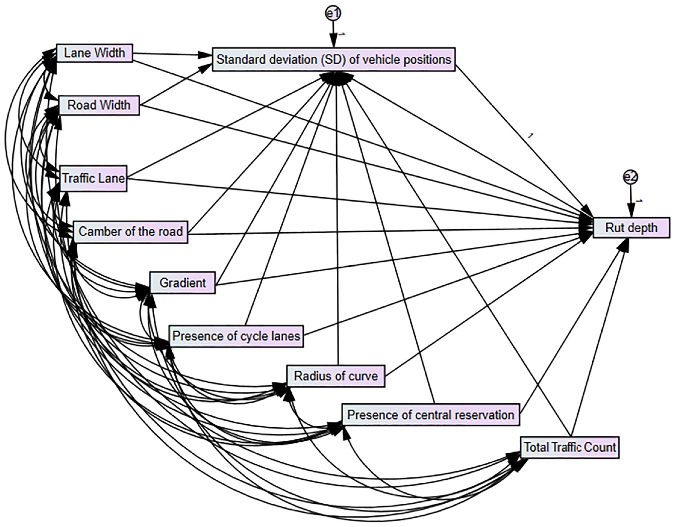
Initial causal diagram of path analysis.
Evaluation
The approach of backward elimination was applied in SEM to remove connections that were deemed to be inconsequential and were represented by arrows. Figure 9 depicts the final version of the model that has been developed. More than 50% of the variation in lateral position can be explained by lane width and road width. In addition, these two groups of variables indirectly influence the rut depth via lateral wander, that is, the standard deviation (SD) of vehicle position. Multiplying the standardized path coefficients allows for estimation of the indirect effects.
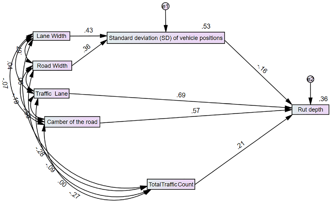
The latest form of path analysis with standardized estimates.
The bidirectional effect of the relationship between rut depth and lateral wander (SD of vehicle position) could not be seen through the model. The reason might lie in the rut depth variable, which has a small variability.
On the other hand, the machine learning model produced four cross-validation models with different hidden layers and neurons. The cross-validated models explained more than 70% (average) of the variation in rut depth, as summarized in Table 1.
Comparison of Model Fit Values
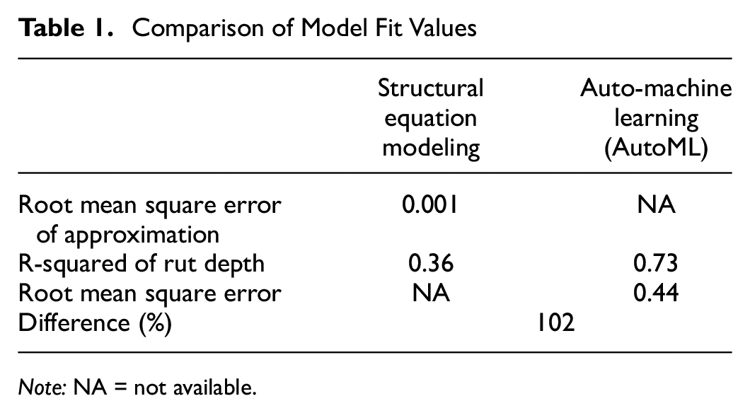
Note: NA = not available.
The root MSE of approximation (RMSEA) was discovered to be less than 0.001 when it came to the SEM. It is advised that it should be less than 0.08 for the model fit values to be considered satisfactory ( 38 ). The root MSE produced by the AutoML model was determined to be 0.44 (on average). That the range of values produced by the model was between 0.2 and 0.5 demonstrates that the model can relatively accurately anticipate the data ( 39 ).
In Figure 10, the chart shows the predicted versus observed results for the test sample, produced by one of the cross-validated models. The highest R-squared value accounted for more than 80% of the variation.
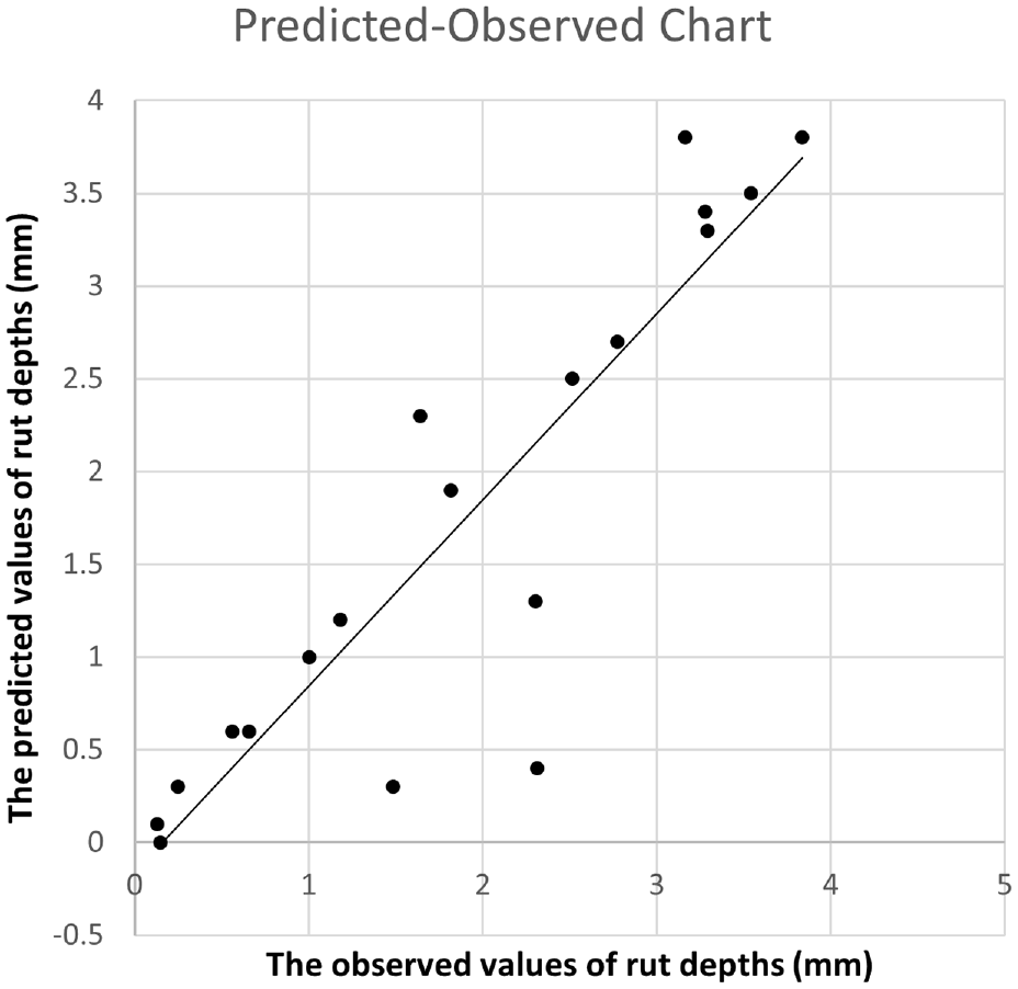
Chart of predicted versus observed results for the best model.
In SEM, standardized path coefficients explain the impacts of variables in the context of model interpretation, summarized in Table 2. For example, an indirect (mediated) effect of road width on rut depth has been calculated to be −0.059 on average. One SD of road width results in a 0.059 SD reduction in rut depth. This is in addition to any direct (unmediated) effect road width may have on rut depth.
Direct and Indirect Effects for Structural Equation Model
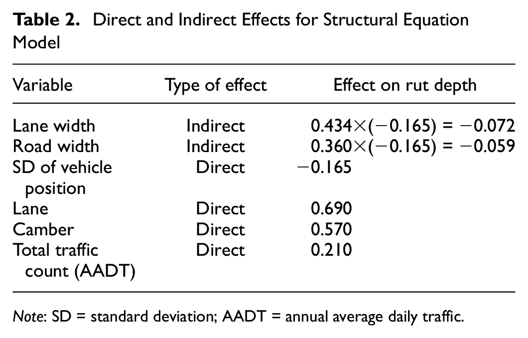
Note: SD = standard deviation; AADT = annual average daily traffic.
The standardized indirect (mediated) effect of road width on rut depth is −0.059. That is, because of the indirect (mediated) effect of road width on rut depth, when road width increases by one SD, rut depth decreases by 0.059 SD. This is in addition to any direct (unmediated) effect road width may have on rut depth.
Table 3 shows the results of the SEM analysis. Several significant associations were discovered. A positive and highly significant relationship was found between lane width and the SD of vehicle position, with an effect of 0.033 and a critical ratio (CR) of 4.624. Road width also had a positive and highly significant effect on SD of vehicle position, with an effect size of 0.017 and a CR of 3.829. Lane was found to significantly influence rut depth with an effect of 1.775 and a CR of 6.637. Interestingly, SD of vehicle position had a significant but negative effect on rut depth, indicating that an increase in SD of vehicle position results in a decrease in rut depth, with an effect of −1.565 and a CR of −1.977. The analysis also revealed a positive and highly significant relationship between camber and rut depth, with an effect size of 0.470 and a CR of 5.272. Lastly, AADT showed a positive and significant effect on rut depth with an effect size of 0.004 and a CR of 2.376.
Results of Structural Equation Model
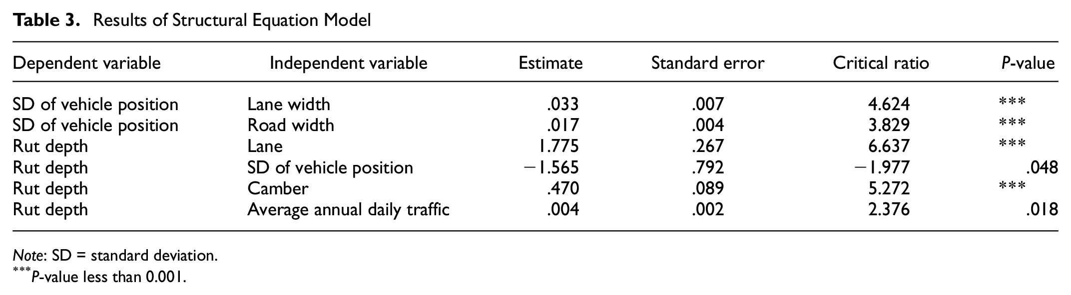
Note: SD = standard deviation.
P-value less than 0.001.
To make sense of the outcomes, the AutoML method employs marginal effect calculation and sensitivity analysis referring to variable importance. The relevance of the most crucial model variables is visualized via a variable importance chart in Figure 11. The result of AutoML is slightly different from SEM. While gradient is not a significant variable in SEM, sensitivity analysis of the AutoML algorithm recognizes that it has a crucial impact on rut depth. The AutoML algorithm seems to have the ability to measure complicated patterns while, in certain circumstances, regression models cannot recognize the complicated feature interactions present.
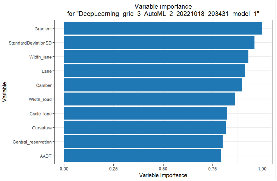
Variable importance chart.
Furthermore, the AutoML algorithm provides the partial dependence plot (PDP), which is a graphical representation showing the marginal effect of one variable on another. The change in the mean response can be used to measure a variable’s influence. PDP assumes independence between the feature for which the PDP is computed and the rest ( 40 ).
The partial dependence plots of the two explanatory variables are displayed in Figure 12. The results of the AutoML model appear to be consistent with the SD of the vehicle position in SEM. Despite this, the AutoML algorithm detected a significant pattern of the gradient variable compared with SEM results. However, the SEM could not demonstrate significant relationships between rut depth and gradient. Gradient has been reported to have one of the most significant influences on the rolling resistance force ( 41 ). It is possible that gradient may affect pavement deterioration via rolling resistance. AutoML recognized the importance of gradient, which might be related to the nonlinear feedback loops between variables. Because of the “black box,” there is no way to resolve this dilemma.
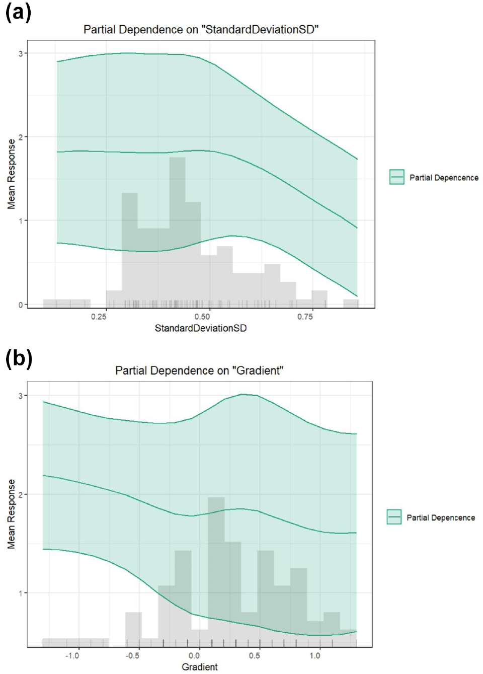
Partial dependence plots of (a) standard deviation and (b) gradient of vehicle position.
Compared with the SEM model, the DNN model demonstrated superior performance. The absence of any underlying assumptions makes it possible to handle nonlinear relationships. However, when it comes to possible interpretations, the black box context is still a concern.
Discussion and Conclusion
These findings were compared with international design standards that use lane width to account for channelization in the design load. The German design standard suggests that for wide lanes, the magnitude of the effect of a 1 m change in width is more modest, although still slightly above the results presented in this study. However, for narrow lanes the magnitude of effect of a change in width is greater. That is, the relationship implicit in the German standards is nonlinear with a large effect at extremely narrow road sections. Unfortunately, any research underpinning this design standard is not stated. The results presented in this study are more in line with the Austrian and German pavement design standards than they are with the current UK standards in that they suggest a continuous relationship between lane width and deterioration. However, the results presented here do not include extremely narrow lane sections, and but include road width, which is not present in either the Austrian or the German design standards.
Our findings suggest that camber seems to be combination of camber, curvature, and longitudinal gradient (as these variables were correlated with each other in the data set). From the data set used in this research, where there was a big camber, there was also a sharp curve. It was still important to keep camber in the model to correct for its effect. This was not the main point to investigate for this research, however, it is an interesting finding that could form the basis of further work to explore the effect of camber alone on the deterioration of pavements.
Pavement design standards and many of the pavement deterioration models in use by practitioners assume linear relationships between vehicle loading, geometries, and rutting. Previous work has suggested that the actual causal mechanisms through which pavements deteriorate may be far more complex, with geometries affecting the way in which people drive, which in turn affects the distribution of loads on the pavement surface, causing deterioration. In the case of the most common form of structural deterioration of flexible asphalt pavements, rutting, it is also suggested that feedback loops might occur between rutting and driver behaviors.
This paper considers two alternative analytical techniques to understanding pavement deterioration: SEM and AutoML. The two approaches had many common results, but with some notable differences. There are advantages and disadvantages to each approach depending on their practical application.
Overall, the DNN approach outperformed SEM in the prediction of rut depth (73% of the variation compared with 36% for SEM). Such approaches may, therefore, be beneficial to highway authorities in predicting the performance of their pavements to help them plan more efficient maintenance schedules. The DNN approach also detected other, potentially important, factors that the SEM did not, especially longitudinal gradient. However, the purpose of this paper is not to interpret the relationships uncovered in the modeling, it is to compare and contrast the alternative modeling approaches to suggest a framework for future analyses in the field of pavement performance. A discussion of the effects of longitudinal gradients and other facts on pavement performance may form the basis of a future publication.
Although the AutoML approach was far superior in the ability to predict rutting, the black box nature of the machine learning approach provides little clear guidance to highway engineers and to design codes as to how pavements could be better designed to minimize rutting and to ensure that pavements achieve their anticipated design life. In this respect, the SEM model is more useful, as it provides evidence as to the causal mechanisms through which rutting occurs. This could allow for more specific design standards to be developed.
In the case study used, the dataset comprised circa 100 locations. Machine learning approaches depend on many observations to be able to recognize patterns and make predictions to high degrees of accuracy, whereas SEM models can usually be created with fewer data points. It is noted that the sample used in this study (100 points) is small compared with the full datasets usually available to a highway authority. In the case of Portsmouth, Colas collects data at more than 100 streets (multiple data points along each street) throughout the city. This larger dataset is not anticipated to present a computational or data storage issue but would require new manual fieldwork to be undertaken if a model for the whole network were developed.
While extrapolation beyond the range of data observed is problematic in both approaches, it is possible that the results of the SEM approach could be used to refine theory as to how rutting occurs, which could then be more generalizable to different contexts and to data beyond the range. Machine learning approaches, however, depend to some extent on similar patterns being recognized in existing datasets to be able to make predictions. Entirely novel contexts are therefore unlikely to be well understood through machine learning.
It is proposed in this paper that both approaches can be utilized in future research into pavement deterioration. Where the underlying relationships between causes and effects are the goal of the research is suggested here that the AutoML approach described in this paper is undertaken first. The findings of the modeling can then be used to guide the researcher in their specification of a SEM model that would be required to represent the causal mechanisms of interest. Where the interest lies purely in predicting the performance of a pavement, given previous/historical data, it is suggested that the AutoML approach alone is the superior method.
Footnotes
Author Contributions
The authors confirm contribution to the paper as follows: study conception and design: M. Ekmekci, R. Sinanmis, L. Woods; data collection: R. Sinanmis; analysis and interpretation of results: M. Ekmekci, L. Woods. R. Sinanmis; draft manuscript preparation: L. Woods. All authors reviewed the results and approved the final version of the manuscript.
Declaration of Conflicting Interests
The author(s) declared no potential conflicts of interest with respect to the research, authorship, and/or publication of this article.
Funding
The author(s) disclosed receipt of the following financial support for the research, authorship, and/or publication of this article: The first author of this paper is fully funded by the Republic of Turkey, Ministry of National Education, Çanakkale Onsekiz Mart University: Study Abroad Program (Sponsorship No. OBS03002).